Estimation of the PM_2.5 and PM₁₀ Mass Concentration over Land from FY-4A Aerosol Optical Depth Data

Abstract

The purpose of this study is to estimate the particulate matter (PM_2.5 and PM₁₀) in China using the improved geographically and temporally weighted regression (IGTWR) model and Fengyun (FY-4A) aerosol optical depth (AOD) data. Based on the IGTWR model, the boundary layer height (BLH), relative humidity (RH), AOD, time, space, and normalized difference vegetation index (NDVI) data are employed to estimate the PM_2.5 and PM₁₀. The main processes of this study are as follows: firstly, the feasibility of the AOD data from FY-4A in estimating PM_2.5 and PM₁₀ mass concentrations were analysed and confirmed by randomly selecting 5–6 and 9–10 June 2020 as an example. Secondly, hourly concentrations of PM_2.5 and PM₁₀ are estimated between 00:00 and 09:00 (UTC) each day. Specifically, the model estimates that the correlation coefficient R² of PM_2.5 is 0.909 and the root mean squared error (RMSE) is 5.802 μg/m³, while the estimated R² of PM₁₀ is 0.915, and the RMSE is 12.939 μg/m³. Our high temporal resolution results reveal the spatial and temporal characteristics of hourly PM_2.5 and PM₁₀ concentrations on the day. The results indicate that the use of data from the FY-4A satellite and an improved time–geographically weighted regression model for estimating PM_2.5 and PM₁₀ is feasible, and replacing land use classification data with NDVI facilitates model improvement.

1. Introduction

With the sustainable development and changes of the economy and society, air pollution, especially particulate matter (PM_2.5) pollution, has been paid more and more attention by the government and people in general. PM_2.5 is a major air pollutant that harms human health [1] and is the fifth major health risk factor of the global burden of disease [2]. At present, the most accurate means of PM_2.5 monitoring are ground-based instruments that can obtain real-time data. However, the ground detection stations only detect air quality in a point-like distribution and cannot cover large areas. Moreover, due to the high cost and maintenance requirements, the stations are mainly distributed in urban areas, making it difficult to achieve full coverage. In addition, site data are greatly affected by special circumstances in a small area near the monitoring station, which makes it difficult to take the overall situation into account.

Compared to ground-based measurements, satellite sensor systems have the advantage of regularly collecting data over large areas, and therefore are able to overcome spatial limitations to a large extent. The study of particulate matter mainly revolves around ground observations, while satellite observations do not directly provide measurements from the ground. Studies have shown that satellite-based aerosol optical depth (AOD) is an ideal substitute for PM_2.5 [3]. With the development of satellite data with increasingly real-time characteristics, PM_2.5 inversion has become a popular research topic. In recent years, more and more researchers have used different AOD data and various models and algorithms to calculate the concentration level of PM_2.5, and good results have been achieved [4,5,6]. However, most AOD products used in current studies are mainly based on existing mature AOD products, such as MODIS [4,7]. PM_2.5 and PM₁₀ products produced using Fengyun (FY-4A) satellite data are not yet officially available, and studies using FY-4A data for particulate matter mass concentration estimation are rare [8].

There are three main approaches to PM_2.5 estimation, including empirical statistical methods, chemical transport model (CTM)-based methods, and vertical correction methods. Based on the vertical distribution and propagation characteristics of AOD, Liu et al. [9] first proposed the global atmospheric chemistry model (GEOS-CHEM) for the Multiangle Imaging SpectroRadiometer (MISR) sensor. Many studies have developed remote sensing inversions of PM_2.5 based on physical mechanism models to obtain PM_2.5 estimates through processes such as particulate size revision, vertical revision, humidity revision, and extinction mass conversion [10,11]. Statistical models are the more current types of methods for estimating PM_2.5. There are mainly five different types of statistical models, including the multiple linear regression model MLR (multiple linear regression), the mixed-effects model MEM (mixed effects model), the GAM (generalised additive model), the GWR (geographically weighted regression model), and machine learning methods.

There is also an increasing number of studies on the estimation of PM₁₀ concentrations. Most of the current studies are similar to PM_2.5 for PM₁₀. Shaw et al. [4] used simple linear regression models and multiple linear regression analysis to calculate the mass concentrations of PM_2.5 and PM₁₀, respectively, and they concluded that the multiple linear regression models were more effective. Wei et al. [12] developed a non-linear empirical model for PM₁₀ based on thirteen PM₁₀ monitoring stations in Xi′an. The correlation coefficient of this non-linear empirical model was nearly three times higher than that of the linear regression model for AOD and PM₁₀. Mixed effects models were employed to regress PM₁₀ measurements [13], and inverse probability weighting was used to account for non-random AOD deficits. The random forest approach was used to estimate PM₁₀ and PM_2.5 concentrations for 2015–2016 in Korea [14]. Hou et al. [15] developed a continuous over-relaxed support vector regression (SOR-SVR) model for predicting PM₁₀ and PM_2.5 and demonstrated that the SOR-SVR model had a better performance of PM₁₀ and PM_2.5 predictions with good generalisation ability. Jiang et al. [16] used a two-stage random forest model to explicitly estimate hourly PM_2.5 concentrations at 1 km spatial resolution in China from March 2018 to February 2019. Chen et al. [17] used linear regression models, geographically and temporally weighted regression models (GTWR), and random forest models without spatio-temporal information (RF) to estimate daily PM_2.5 concentrations for 2016–2018 based on ground-based PM_2.5 and meteorological variable data. Wei et al. [18] developed a new spatio-temporal random forest (STRF) model to generate high spatial resolution (1 km) PM_2.5 concentrations over China using the Moderate Resolution Imaging Spectroradiometer (MODIS) AOD product.

Most machine learning models have the overfitting problem [19,20,21]. Least squares and GWR models were used to estimate PM_2.5 and PM₁₀ in China [12,22], with GWR models being significantly more accurate than linear regression models. GTWR models with spatio-temporal weighting have performed better than models with spatial (i.e., GWR) or temporal (i.e., TWR) weighting only [23,24]. You et al. [25] used the MODIS 3 km resolution Aerosol Optical Depth (AOD) product to create a nationwide geographically weighted regression (GWR) model to estimate ground-level PM_2.5 concentrations in China and considered fire emissions detected by MODIS fire counts in the model development process. Yang et al. [23] used a proposed geographically and temporally weighted regression (GTWR) model to generate ground-level 500 m resolution PM_2.5 concentrations with the AOD obtained from satellites. In recent years, several researchers have used AOD data to estimate PM for Asian regions, especially China. Wei et al. [26] found that high PM₁₀ concentrations occur in northwestern China (e.g., the Tarim Basin) and the northern plains of China by generating a PM₁₀ dataset for China from 2015 to 2019, which is consistent with the areas where PM₁₀ exceeds 100 μm/m³ in this study. Yang et al. [27] investigated the relationship between PM_2.5 and AOD in Chinese cities at different temporal and regional scales and summarised the temporal and spatial patterns of PM_2.5/AOD ratios and correlations. By investigating the relationship between PM_2.5 and HIMAWARI (AHI) AOD in the mainland of China, Xu et al. [28] found that the correlation between PM_2.5 and AHI AOD increased significantly with the number of AOD retrievals in a day, and the relationship between PM_2.5 and AOD changed with time. Therefore, AOD of high temporal resolution is of great relevance for PM_2.5 estimation. Wang et al. [29] used a multi-temporal approach to retrieve 3 km resolution aerosol optical depth (AOD) and fine mode fraction (FMF) from geostationary ocean colour imager (GOCI) data. Then, they used them to estimate PM_2.5 concentrations in the Beijing area. Wang et al. [30] estimated ground-level PM_2.5 concentrations in Taiwan, using a 100 m resolution AOD obtained from Chinese OF-1 WFV imagery, and the correlation R between the observed and calculated PM_2.5 results were 0.551 and 0.655, respectively. Park et al. [5] used three schemes (i.e., G1, A1, and A2) to estimate spatially continuous AOD, PM₁₀, and PM_2.5 concentrations for East Asia using geostationary ocean colour imager (GOO)-based data, which can be used for spatially continuous AOD and PM under all sky conditions estimation. Zhao et al. [31] estimated PM_2.5 concentrations in the Beijing–Tianjin–Hebei region from a developed random forest model and found that the one-day lagged boundary layer height made the most significant contribution to the model. Yang et al. [32] studied the relationship between PM_2.5 and AOD using AOD data obtained from MODIS, and found that the meteorological influence on PM and AOD was strong in June. Li et al. [33] estimated daily PM_2.5 concentrations in the Beijing–Tianjin–Hebei region of northern China during 2017 using a mixed-effects model. The impact of the spatial resolution and sampling frequency of the AOD on PM_2.5 prediction was then assessed. Xu et al. [34] introduced NDVI into the corrected regression model to map the seasonal and annual mean distribution of PM_2.5 concentrations in Beijing from 2014 to 2016, and the quality of the corrected regression model was improved significantly.

Jiang et al. [35] used the PMRS (physical PM_2.5 remote sensing) method with FY-4A data to estimate surface atmospheric particulate matter concentrations with R² up to 0.39 for the Beijing–Tianjin–Hebei region. Mao et al. [8] used the random forest algorithm and FY-4A to estimate PM_2.5 in China on an hour-by-hour basis with an average r² close to 0.92 and an RMSE of 10.0 μg/m³.

This paper employs the IGTWR model proposed by Xue et al. [36] to estimate PM₁₀ and PM_2.5 mass concentrations using data from the Chinese Fengyun-4 satellite. However, unlike previous studies, where the parameters used by previous models in defining the generalised distances were land classification data, this study uses NDVI as a proxy for land classification data. The framework of this paper is given below. Section 3 presents the detailed algorithm, including the definition of the generalised distance and the choice of window width. Section 4 presents the results of the algorithm, as well as the validation results and the variation of PM_2.5 and PM₁₀. This section also analyses possible reasons for the differences in the results resulting from the definition of the generalised distances for the two factors. Conclusions are given in Section 5, and future plans are discussed in this section.

2. Data

2.1. Study Area

The study area is the mainland of China, except for the smaller islands in the South China Sea (Figure 1). The vast area includes a variety of topographical features such as plains, plateaus, mountains, and hills, adding to the difficulty of PM_2.5 and PM₁₀ estimates.

2.2. PM_2.5 and PM₁₀ Data

The ground detection data of PM_2.5 and PM₁₀ are from the National Real-time Air Quality Publishing Platform (http://106.37.208.233:20035/ (accessed on 1 July 2020)). Monitoring sites from across the country are employed to collect data, including hourly monitoring values for PM_2.5 mass concentrations and PM₁₀ mass concentrations. These include data from over 1600 sites, and the number of sites grows over time. The measurement data for the site is collected every hour, and data with null measurements are removed. The ground monitoring value provides the basis for the establishment of the model and the verification of the results. Additionally, 6131 measurements of PM₁₀ and 6113 measurements of PM_2.5 were used for model validation.

2.3. Fengyun-4 (FY-4A) Data

The FY-4A satellite was launched on 11 December 2016. Fengyun-4 is a China′s new generation of geostationary meteorological satellite, which has greatly enhanced the capability of monitoring, warning, and forecasting of high impact weather events [38].

Its main payload is the Advanced Geosynchronous Radiation Imager (AGRI). It has 14 spectral bands that are quantised to 12 bits per pixel and sampled at 1 km at the nadir in the visible (VIS), 2 km in the near-infrared (NIR), and 4 km in the remaining IR spectral bands (compared with 1.25 km for VIS, no NIR, and 5 km for IR of FY-2). The archived L1 dataset of FY-4A is available on the National Satellite Meteorological Center (NSMC) satellite data server website (http://satellite.nsmc.org.cn (accessed on 1 July 2020)).

Xia et al. [39] developed a grid point statistical interpolation (GSI)-based data assimilation system and successfully assimilated FY-4A aerosol optical depth (AOD) data for the first time. AOD data are obtained via the AGRI imager on the FY-4A, together with a joint retrieval algorithm for surface reflectance and aerosol optical thickness using the algorithm proposed and implemented by She et al. [7]. Therefore, daily AOD data is obtained from 00:00 to 09:00 (UTC).

2.4. Relative Humidity

Relative humidity (RH) is the percentage of water vapour pressure in the air compared to the saturation water vapour pressure at the same temperature. Ground stations measure particulate concentrations by drying the sampling air stream to remove the effect of moisture on particulate mass concentrations. Obviously, atmospheric humidity also has a significant effect on pollutants in the air, so relative humidity is also used as one of the independent variables in the model. Relative humidity data are obtained from “ERA5 hourly data on single levels from 1979 to present” data (https://cds.climate.copernicus.eu/cdsapp#!/dataset/reanalysis-era5-pressure-levels?tab=overview (accessed on 1 July 2020)). The time resolution of RH data is 1 h. The data are hourly raster data at a resolution of 0.25° × 0.25°. Additionally, linear interpolation is used to obtain data at 1 km resolution.

2.5. (Planetary) Boundary Layer Height

The planetary boundary layer (PBL), also known as the atmospheric boundary layer or pedosphere, can be defined as the lowest part of the atmosphere, typically ranging anywhere between 100 m and 2000 m above the planetary surface, and its behaviour is directly influenced by its contact with a surface. Boundary layer height has a significant effect on atmospheric particulate matter concentrations [40]. The boundary layer height data used in this study are also from ERA5 of ECMWF, the fifth generation of ECMWF′s atmospheric reanalysis of the global climate (https://cds.climate.copernicus.eu/cdsapp#!/dataset/reanalysis-era5-single-levels?tab=overview (accessed on 1 July 2020)). The data are hourly raster data at a resolution of 0.25° × 0.25°. In the data pre-processing, linear interpolation was used to obtain 1 km resolution boundary layer height data for the study area.

2.6. Land Use Type

Land use classification data of China in 2020 is collected from the Resource and Environment Data Cloud Platform (http://www.resdc.cn/ (accessed on 1 July 2020)). The data are based on the Landsat TM image of the United States Landsat, which is generated by human visual interpretation with 1 km spatial resolution.

The data include six primary types of arable land, forest land, grassland, water, residential land, and unused land, and 25 secondary types. The values in the raster data are their values, which can be used as the raw data for the input, and the specific classification numbers and names are shown in

Table 1. The land use types of LUCC classification system over China [37].

Primary Types		Secondary Types
Number	Designation	Number	Designation
1	Cultivated land	11	Paddy field
		12	Dry land
2	Forest	21	Woodland
		22	Shrub wood
		23	Sparse woodland
		24	Other woodlands
3	Lawn	31	High-coverage grassland
		32	Medium-coverage grassland
		33	Low-coverage grassland
4	Water area	41	Channel
		42	Lake
		43	Reservoir pond
		44	Permanent glacier and snow
		45	Tidal flat
		46	Beach land
5	Urban, rural, industrial, mining and residential land	51	Urban land use
		52	Rural settlements
		53	Other construction land
6	Unused land	61	Sand
		62	Gobi
		63	Saline alkali soil
		64	Swamp land
		65	Bare land
		66	Bare rock texture
		67	Other
9		99	undefined

.

2.7. MODIS NDVI Data

The global MOD13A2 data are available at a spatial resolution of 1 km every 16 days as a gridded level-3 of the sinusoidal projection. As vegetation indices can be used as products to show land cover and land cover change, the normalised vegetation indices from the MOD13A2 data are used in this paper as a proxy for the land use data in the IGTWR model. These products can be obtained from the website https://ladsweb.modaps.eosdis.nasa.gov/missions-and-measurements/products/MOD13A2#overview (accessed on 1 July 2020).

3. Methods

There have been many studies on geographic data, and the prevailing view is that geographic data are influenced by both their geographical location and time. Hence, Huang et al. [41] propose a geographic time-weighted regression model.

$$y_i={\mathsf{\beta }}_0(u_0,v_0,t_0)+{\displaystyle \sum _{k=1}^d{\mathsf{\beta }}_k(u_0,v_0,t_0)}{x}_{ik}+{\epsilon }_i, i=1,2,\dots ,n.$$

(1)

where i is the observation point (i = 1, 2, ..., n, n is the total number of observation points); k is the model parameter (k = 1, 2, ..., d, d is the total number of parameters); y_i is the estimated parameter, and x_ik represents the independent variable of k at point i; β is the coefficient; u₀, v₀, and t₀ represent longitude, latitude and date, respectively; and ε_i represents the random error.

PM_2.5 concentration levels are not only influenced by time and space but are also linked to subsurface data within the study area. In the study from Xue [36], an improved geographically and temporally weighted regression (IGTWR) model was thereby established (Equation (2)). AOD, RH, and BLH were used as parameter inputs to the model. The relationships between different sample sites are described by temporal (day and hour), spatial (longitude and latitude), and underlying surface data (land use data).

$$y_i={\mathsf{\beta }}_0(u_0,v_0,d_0,h_0,l_0)+{\mathsf{\beta }}_1(u_0,v_0,d_0,h_0,l_0)AO{D}_i+{\mathsf{\beta }}_2(u_0,v_0,d_0,h_0,l_0)R{H}_i+{\mathsf{\beta }}_3(u_0,v_0,d_0,h_0,l_0)BL{H}_i+{\epsilon }_i, i=1,2,\dots ,n.$$

(2)

In the equations, 𝑢₀, 𝑣₀, 𝑑₀, ℎ₀, and l₀ represent longitude, latitude, day, hour, and land use classification data, respectively. d refers to the number of independent variables (FY-4A AOD, relative humidity, and boundary layer height) in this model, and d = 3; i denotes the observation point, i = 1, 2, ..., n, where n is the total number of observation points.

The limited number of classification categories for land use data (a total of 26 land categories are in the LUCC) makes it difficult to quantify the complexity of the subsurface data. Therefore, NDVI was used instead of land use data for the modelling in this paper.

Equation (2) can be written as Equation (3), and vi₀ refers to NDVI:

$${\mathsf{y}}_i={\beta }_0(u_0,v_0,d_0,h_0,v{i}_0)+{\displaystyle \sum _{k=1}^d{\beta }_k}(u_0,v_0,d_0,h_0,v{i}_0)x_{ik}+{\epsilon }_i,i=1,2,\dots ,n$$

(3)

In the regression process, different stations have different weights, so weighting coefficients were calculated using latitude, longitude, date, hour, and NDVI, which were referenced in the model. PM_2.5 and PM₁₀ concentrations within the study area were fitted using AOD, RH, and BLH as independent variables, combined with the weighting coefficients, so that the objective function can be expressed as Equation (4).

$$f={{\displaystyle \sum _{i=1}^n\left[y_i-{\mathsf{\beta }}_0(u_0,v_0,d_0,h_0,v{i}_0)-{\displaystyle \sum _{k=1}^d{\mathsf{\beta }}_k(u_0,v_0,d_0,h_0,v{i}_0)x_{ik}}\right]}}^2{\omega }_i(u_0,v_0,d_0,h_0,v{i}_0).$$

(4)

The estimated PM_2.5 or PM₁₀ concentration Y at (u₀, v₀, d₀, h₀, vi₀) is given in Equation (5) below:

$$\widehat{y}(u_0,v_0,d_0,h_0,v{i}_0)=x_0{}^T\widehat{\mathsf{\beta }}(u_0,v_0,d_0,h_0,v{i}_0)=x_0{}^T{\left[X^{T}W(u_0,v_0,d_0,h_0,v{i}_0)X\right]}^{-1}{X}^{T}W(u_0,v_0,d_0,h_0,v{i}_0)Y.$$

(5)

Therefore, the PM_2.5 or PM₁₀ concentration at (u_i, v_i, d_i, h_i, vi_i) is:

$$\widehat{y}(u_i,v_i,d_i,h_i,v{i}_i)=x_i{}^T\widehat{\mathsf{\beta }}(u_i,v_i,d_i,h_i,v{i}_i)=x_i{}^T{\left[X^{T}W(u_i,v_i,d_i,h_i,v{i}_i)X\right]}^{-1}{X}^{T}W(u_i,v_i,d_i,h_i,v{i}_i)Y.$$

(6)

The model also requires the determination of weighting factors based on spatio-temporal data and land use type data. The distance between the estimated point (u₀, v₀, d₀, h₀, vi₀) and any other observed sample data (u_i, v_i, d_i, h_i, vi_i) is first defined according to:

$$d_{0i}=\sqrt{\lambda [{(u_0-u_i)}^2+{(v_0-v_i)}^2]+\mu [{(d_0-d_i)}^2+{(h_0-h_i)}^2]+\phi [{(v{i}_0-v{i}_i)}^2]}$$

(7)

where $\lambda$, $\mu$, and $\phi$ represent the weighting coefficients, and the weighting function is expressed as a Gaussian function as:

$$\begin{array}{lll}{\omega }_i(u_0,v_0,d_0,h_0{\mathit{vi}}_0) & = \mathit{exp}(-\frac{d_{\mathit{oi}}^2}{h_{\mathit{STL}}^2})& \\ & = \{-\frac{\lambda [{(u_0-u_i)}^2+{(v_0-v_i)}^2]+\mu [{(d_0-d_i)}^2+{(h_0-h_i)}^2]+\phi \left[{({\mathit{vi}}_0-{\mathit{vi}}_i)}^2\right]}{h_{\mathit{STL}}^2}\}\\ & = \left\{\right(-\frac{\lambda [{(u_0-u_i)}^2+{(v_0-v_i)}^2]}{h_{\mathit{STL}}^2}+\frac{\mu [{(d_0-d_i)}^2+{(h_0-h_i)}^2]}{h_{\mathit{STL}}^2}+\frac{\phi \left[{({\mathit{vi}}_0-{\mathit{vi}}_i)}^2\right]}{h_{\mathit{STL}}^2}\left)\right\}\\ & = \{-(\frac{{(u_0-u_i)}^2+{(v_0-v_i)}^2}{h_{\mathit{STL}}^2}+\frac{{(d_0-d_i)}^2+{(h_0-h_i)}^2}{h_{\mathit{STL}}^2}+\frac{{({\mathit{vi}}_0-{\mathit{vi}}_i)}^2}{h_{\mathit{STL}}^2}\left)\right\}\\ & = \mathit{exp}\{-(\frac{{\left(d_{\mathit{oi}}^s\right)}^2}{h_{\mathit{s}}^2}\left)\right\}\times \mathit{exp}\{-(\frac{{\left(d_{\mathit{oi}}^T\right)}^2}{h_{\mathit{T}}^2}\left)\right\}\times \mathit{exp}\{-(\frac{{\left(d_{\mathit{oi}}^L\right)}^2}{h_{\mathit{L}}^2}\left)\right\}\\ & = {\omega }_i^s(u_0,v_0)\times {\omega }_i^T(d_0,h_0)\times {\omega }_i^L\left({\mathit{vi}}_0\right)\end{array}$$

(8)

where h_STL, h_S, h_T and h_L represent spatial, temporal and land use bandwidths, respectively; and ${\omega }_i^s(u_0,v_0)$, ${\omega }_i^T(d_0,h_0)$ and ${\omega }_i^L(v{i}_0)$ are weights.

The cross-validation method is employed to select the best bandwidth that provides the smallest residuals.

$$CV(h_S,h_T,h_L)={\displaystyle \sum _{i=1}^n{[y_i-{\widehat{y}}_i(h_S,h_T,h_L)]}^2},$$

(9)

$$CV({\widehat{h}}_S,{\widehat{h}}_T,{\widehat{h}}_L)=\min \left(CV(h_S,h_T,h_L)\right).$$

(10)

4. Results

The improved IGTWR model is applied to the FY-4A data to estimate hourly PM_2.5 and PM₁₀ mass concentrations for 5–6 and 9–10 June 2020 in mainland China. In this section, the validation of PM measurements were focused on assessing the performance of the improved model. In addition, the daily variation of PM was analysed, and the sudden occurrence of heavy pollution in clean areas such as Xinjiang in June 2020 was explored.

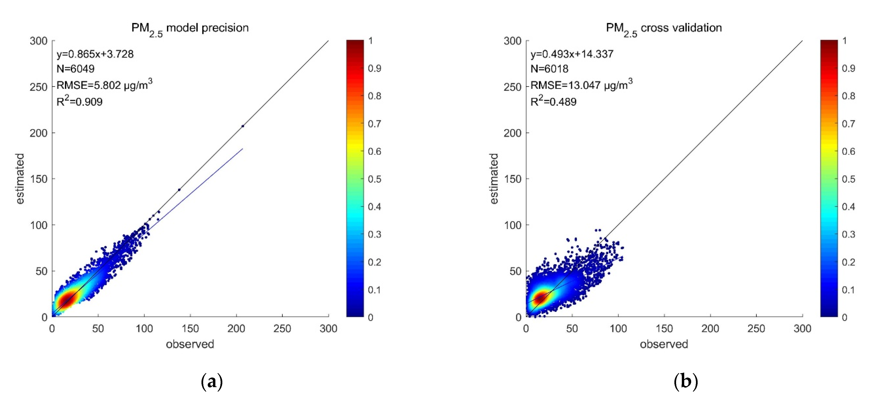
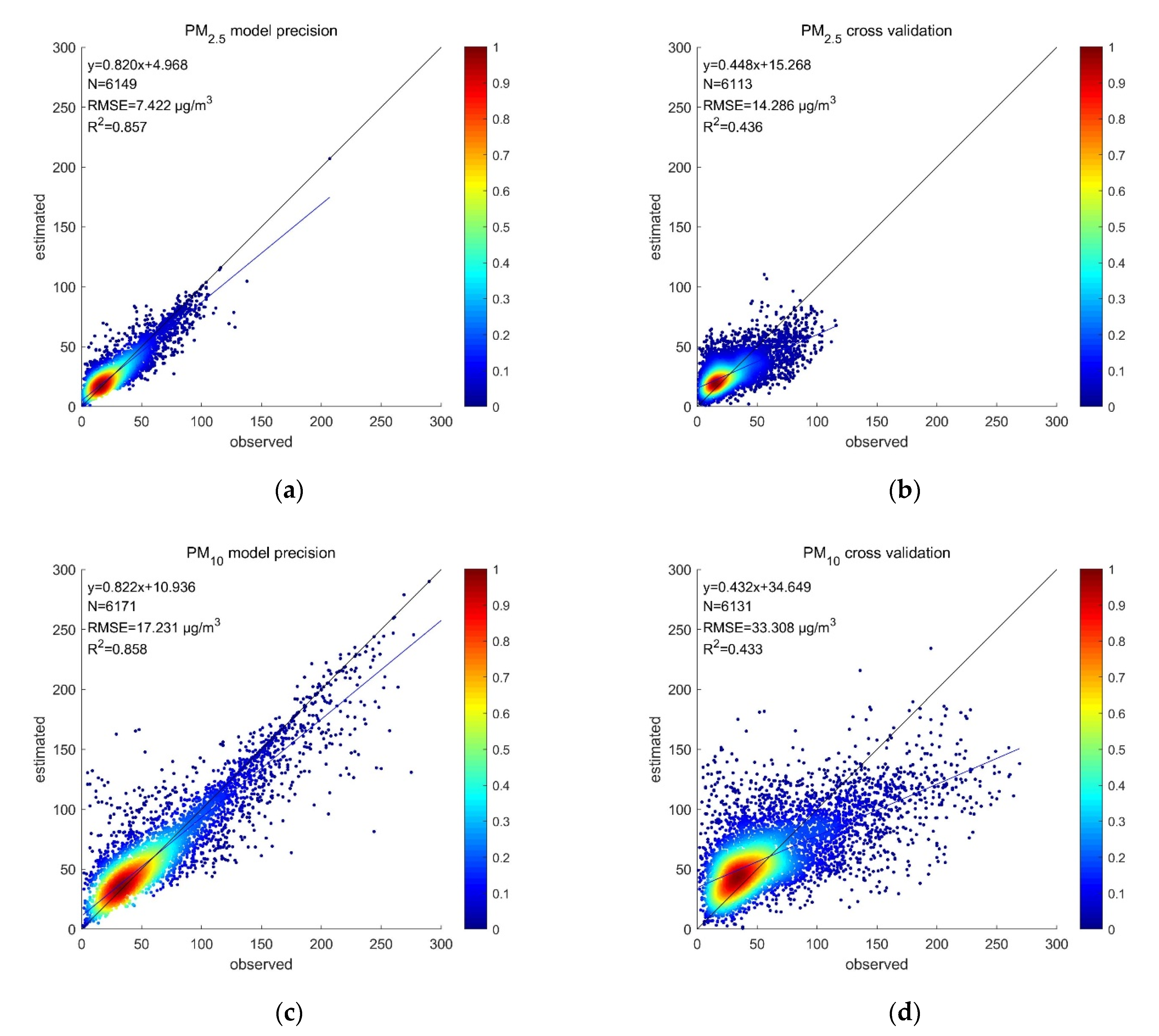
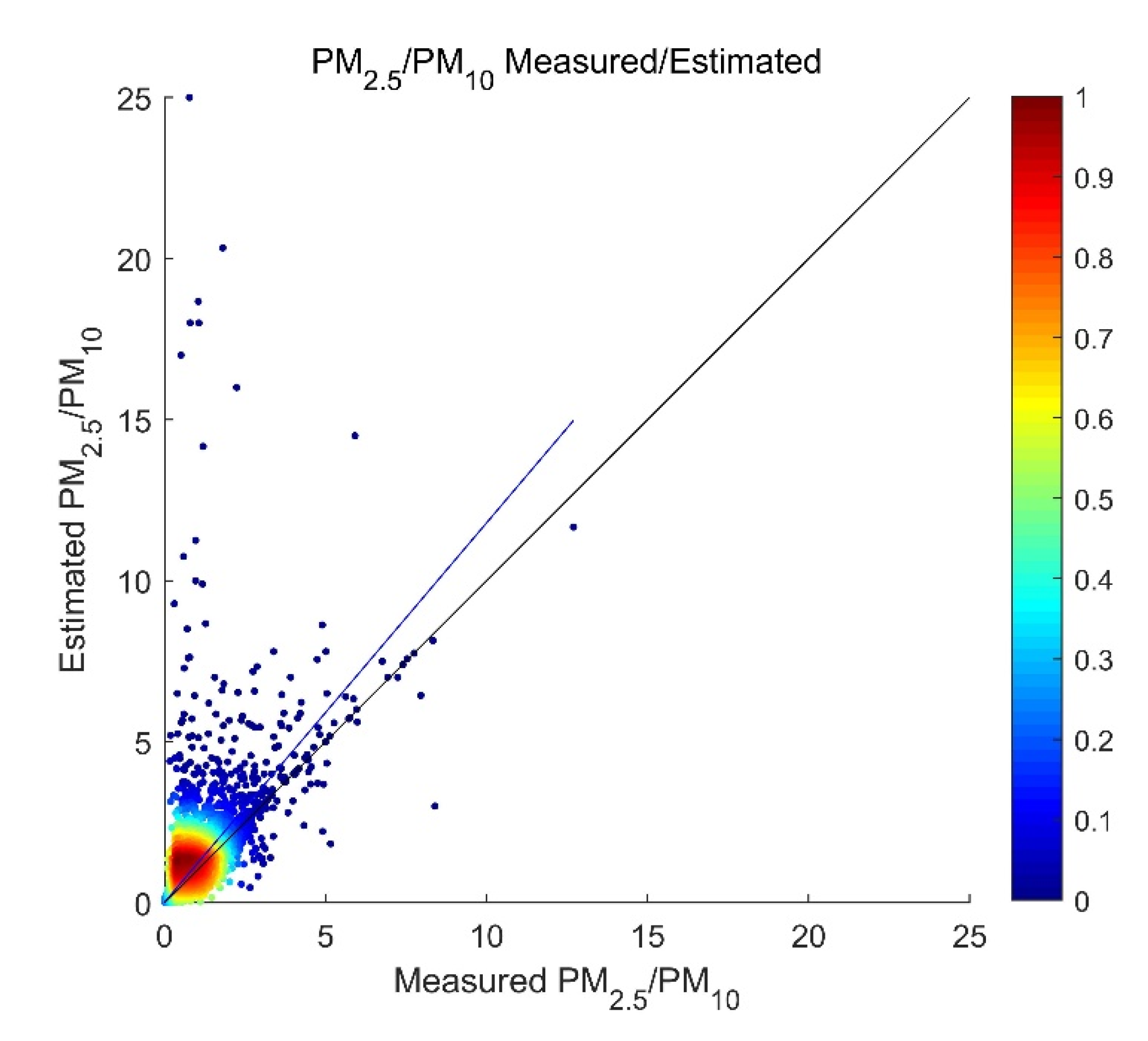
4.1. Evaluation of IGTWR Model Applied to FY-4A

In this study, the IGTWR model was used to estimate hourly PM_2.5 and PM₁₀ mass concentrations during the daytime in China on 5–6 and 9–10 June 2020. Hourly FY-4A AOD from UTC 00:00 to UTC 09:00 (LST 08:00 to LST 17:00), relative humidity, and boundary layer height were employed as input parameters. Longitude, latitude, date, hour, and NDVI were used to calculate the regression weights. The 6049 sample points were used to construct the modelling set for the IGTWR model. The model fitting performance is shown in Figure 2 (left). A ten-fold cross-validation approach was used to assess model performance [42]. Then, 6049 sample points were divided evenly into ten parts. One part was used for validation, and the remaining nine parts were used for training; the process was repeated ten times. Figure 2 shows the cross-validation results (right). For a sample of 6049 points in ten hours, the correlation coefficient R² value between predicted and observed PM_2.5 was 0.909, and the root mean squared error (RMSE) of the model fitting was only 5.802 μg/m³. In the scatter plot of measured versus predicted values, the points were distributed around a 1:1 line. The cross-validated R² was 0.489, and the RMSE was 13.047 μg/m³, which was only 7.245 μg/m³ higher than the RMSE of the model fitting. The slope of the fitting line of the measured–predicted PM_2.5 scatter plot was 0.493. This indicates that PM_2.5 was overestimated for concentrations below 30 μg and underestimated for concentrations above this for short periods. For a sample of 6070 points in ten hours, the R² value between predicted and observed PM₁₀ was 0.915, and the RMSE of the model fitting was only 12.939 μg/m³. In the scatter plot of measured versus predicted values, the points were distributed around a 1:1 line. The cross-validated correlation coefficient R² was 0.498, and the RMSE was 29.779 μg/m³, which was only 16.84 μg/m³ higher than the RMSE of the model fitting. The slope of the fitting line of the measured-predicted PM₁₀ scatter plot was 0.484. This indicates that PM₁₀ was overestimated for concentrations below 60 μg and underestimated for concentrations above this for short periods.

For a more intuitive comparison with the previous model, the same data are used for the calculations, except that land use data is used instead of NDVI. Figure 3 shows the scatter plots for model fitting results and tenfold cross-validation results for PM_2.5 and PM₁₀. For a sample of 6149 points in ten hours, the correlation coefficient R² value between predicted and observed PM_2.5 was 0.857, and the root mean squared error (RMSE) of the model fitting was only 7.422 μg/m³. In the scatter plot of measured versus predicted values, the points were distributed around a 1:1 line. The cross-validated R² was 0.436, and the RMSE was 14.286 μg/m³. The slope of the fitting line of the measured-predicted PM_2.5 scatter plot was 0.448. For a sample of 6171 points in ten hours, the R² value between predicted and observed PM₁₀ was 0.858, and the RMSE of the model fitting was only 17.231 μg/m³. In the scatter plot of measured versus predicted values, the points were distributed around a 1:1 line. The cross-validated correlation coefficient R² was 0.433, and the RMSE was 33.308 μg/m³. The slope of the fitting line of the measured–predicted PM₁₀ scatter plot was 0.432.

The difference in the validation results indicates that the model using NDVI to participate in the definition of the generalised distance has a higher R² than the previous model. Although this improvement is not particularly significant, it still illustrates the significance of the improved model work.

Figure 4 shows the measured and estimated PM_2.5/PM₁₀ ratios. In the study area, the mass concentration of PM₁₀ is generally higher than the mass concentration of PM_2.5. In the scatter plot, the points are mostly distributed above a 1:1 line, which indicates that the measured PM_2.5/PM₁₀ ratio is usually somewhat higher than the estimated ratio.

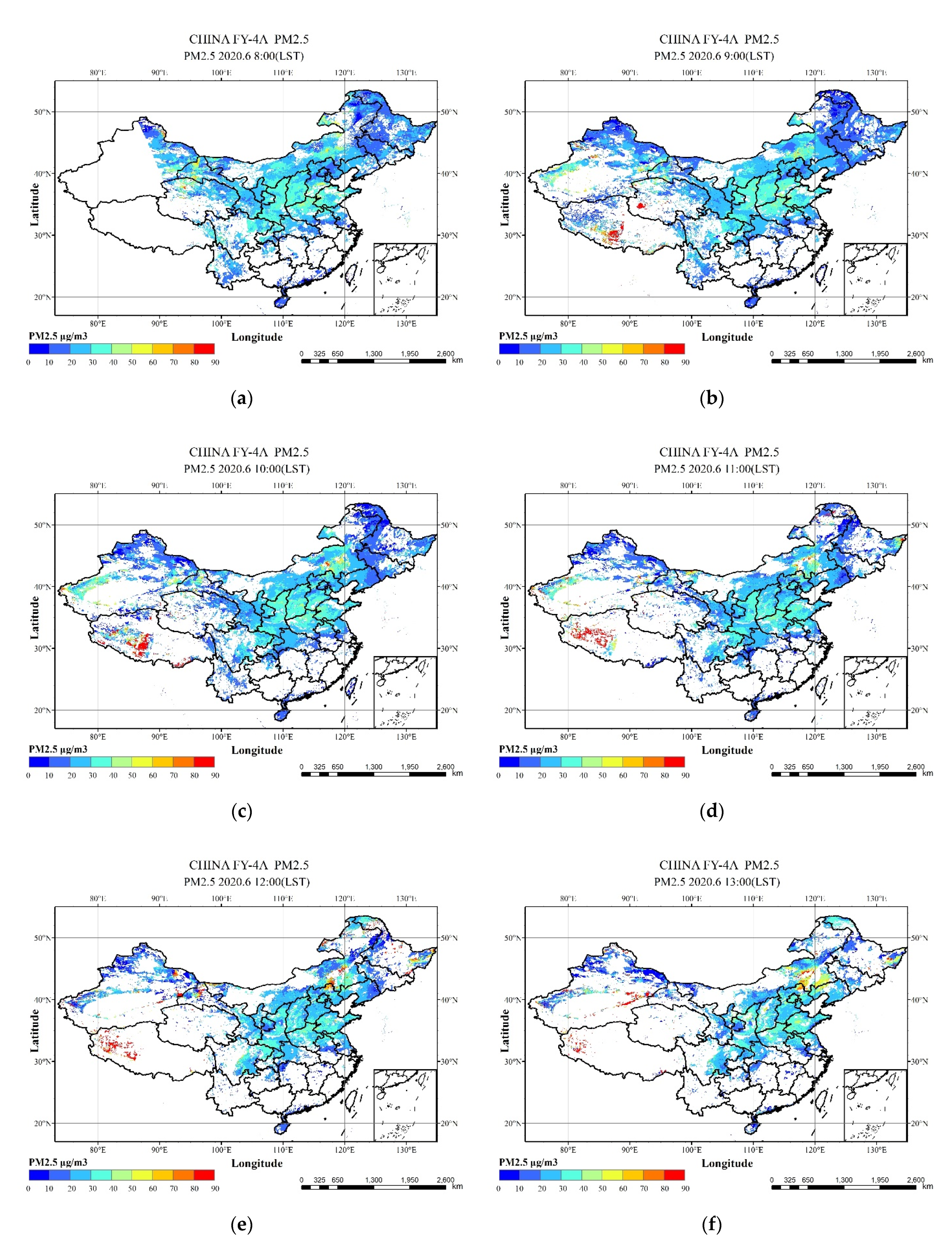
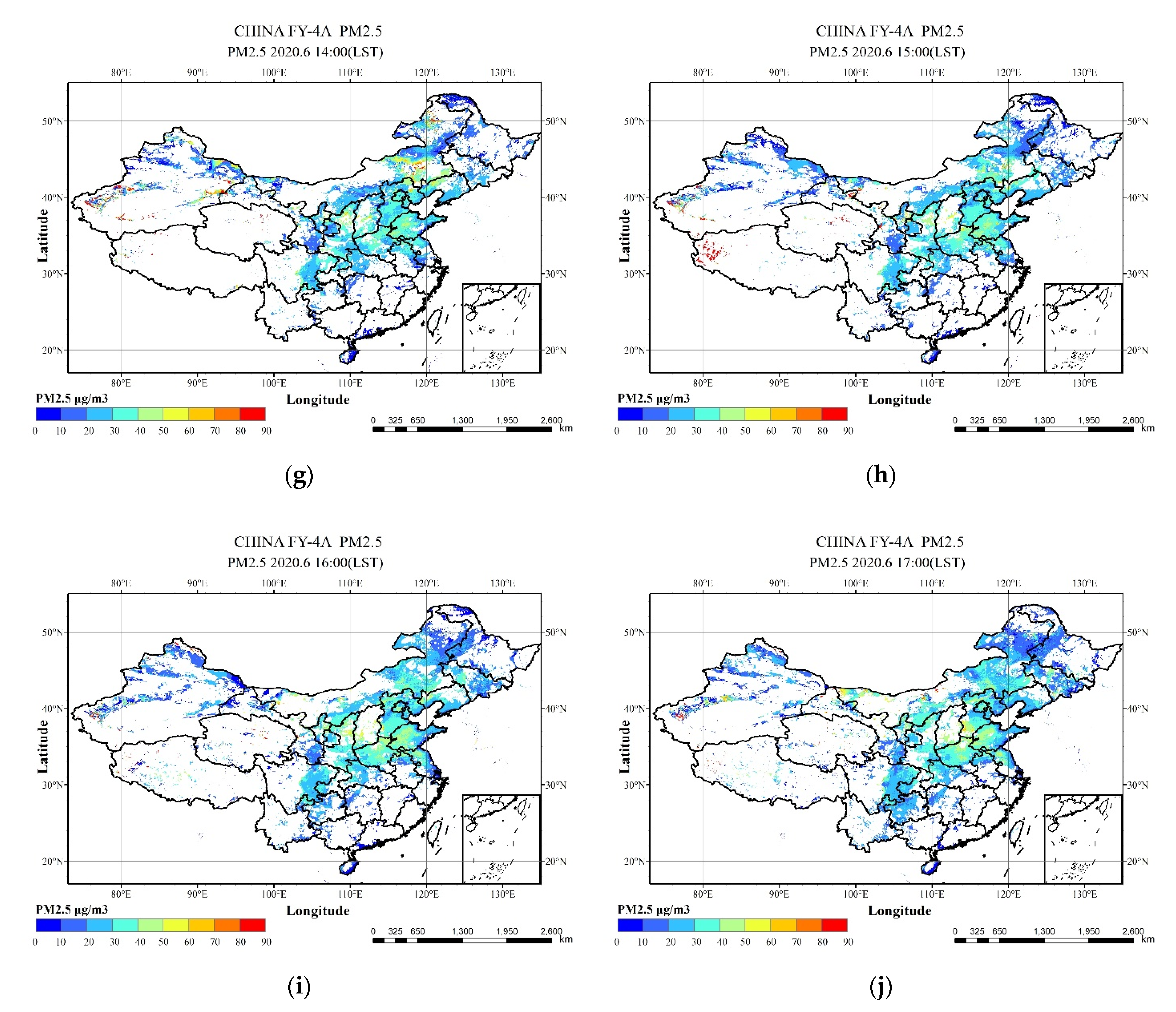
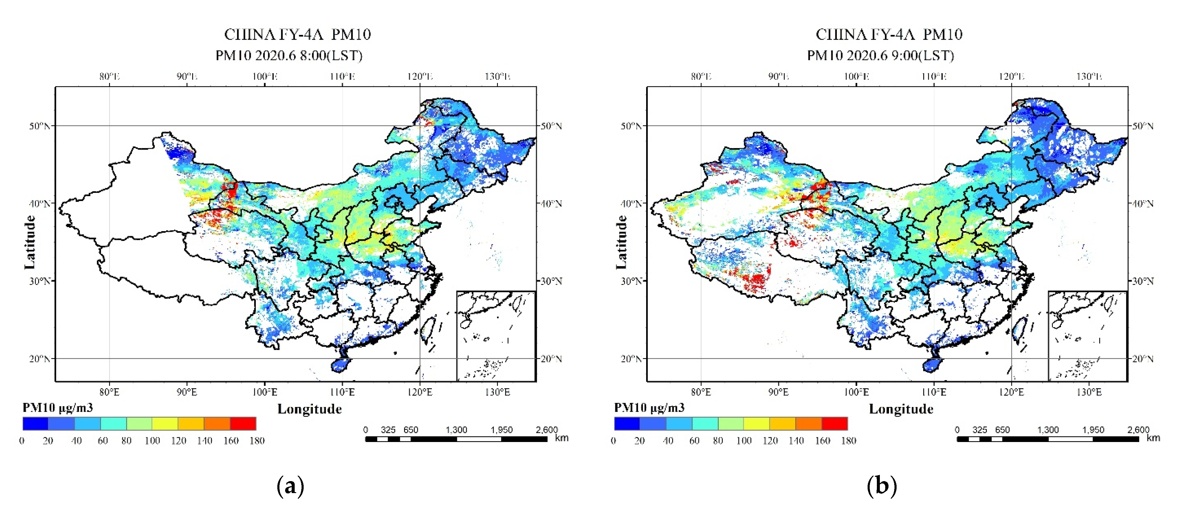
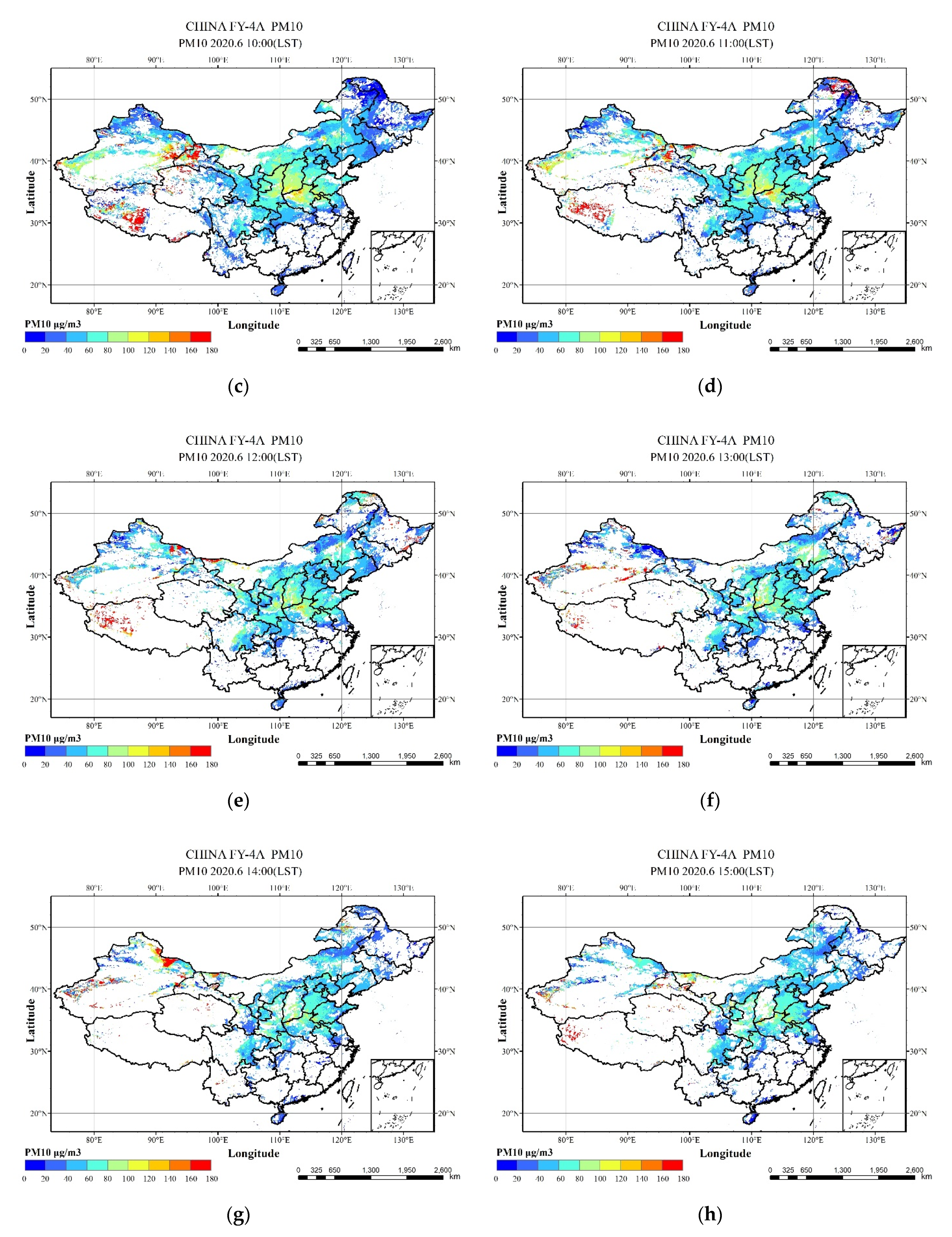
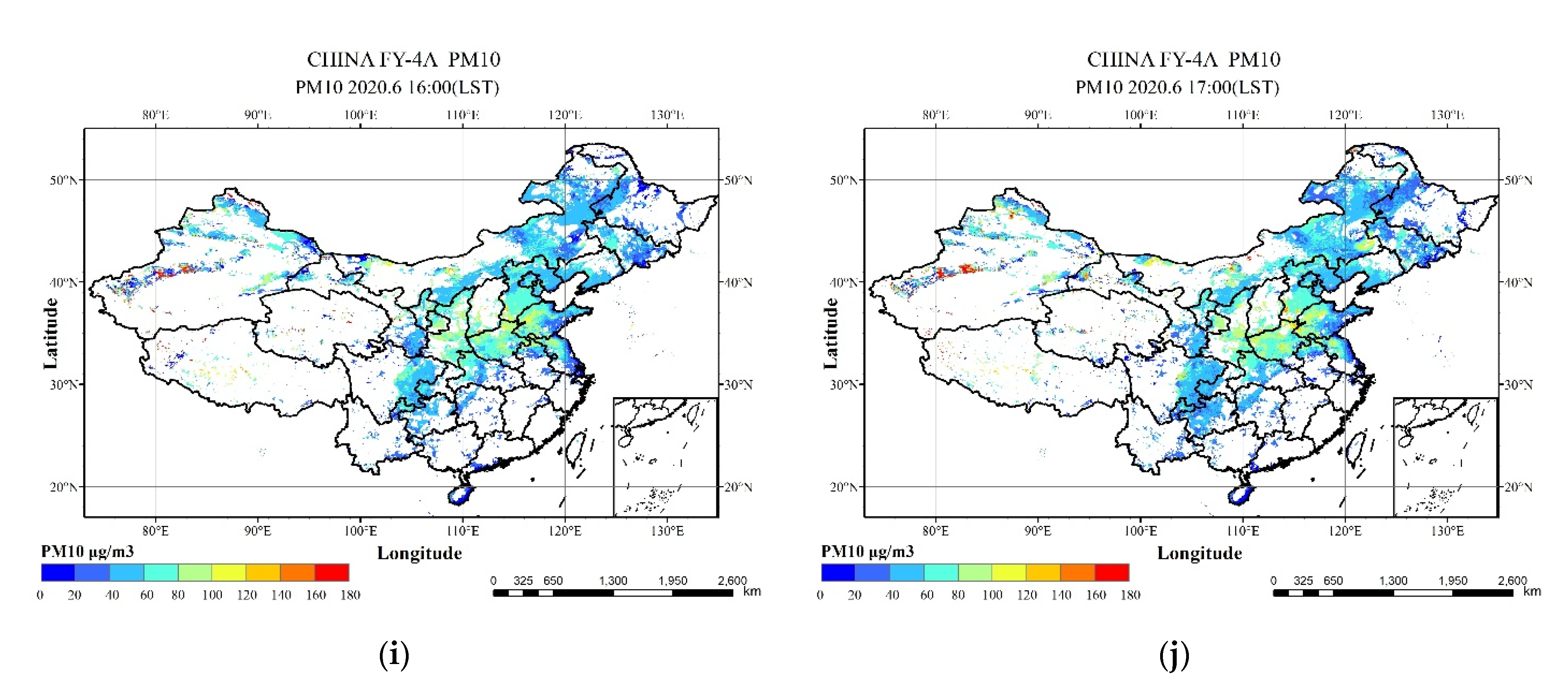
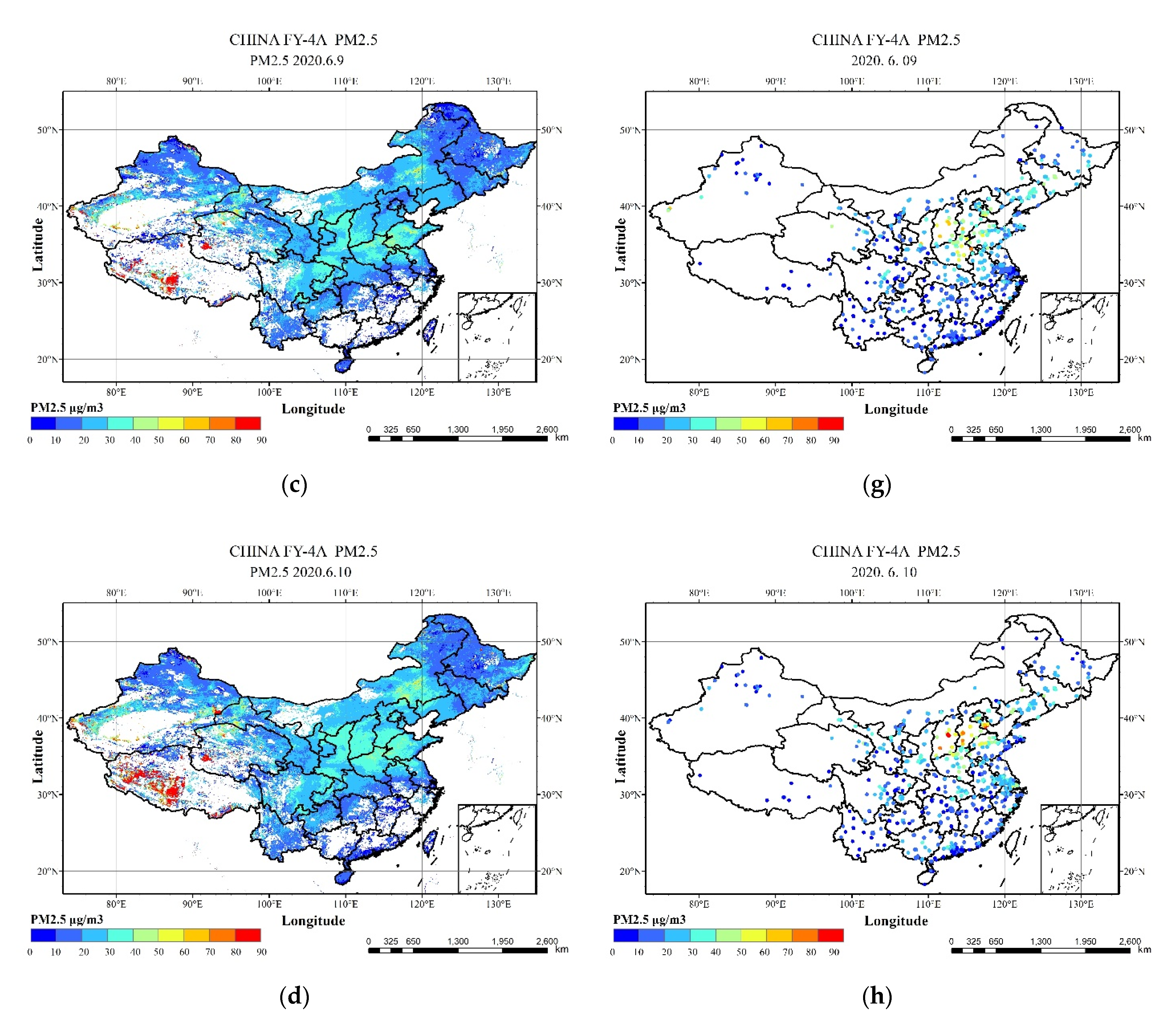
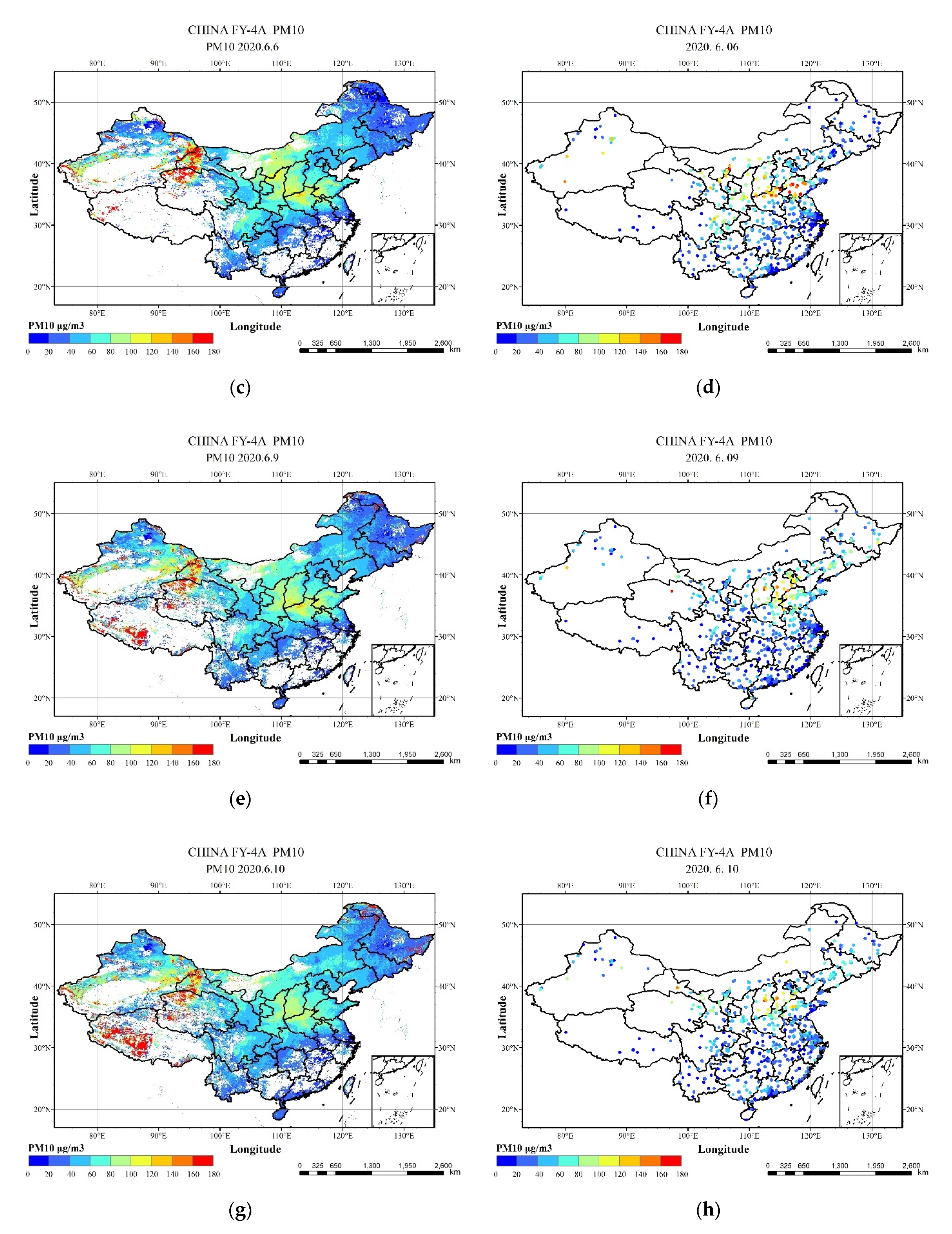
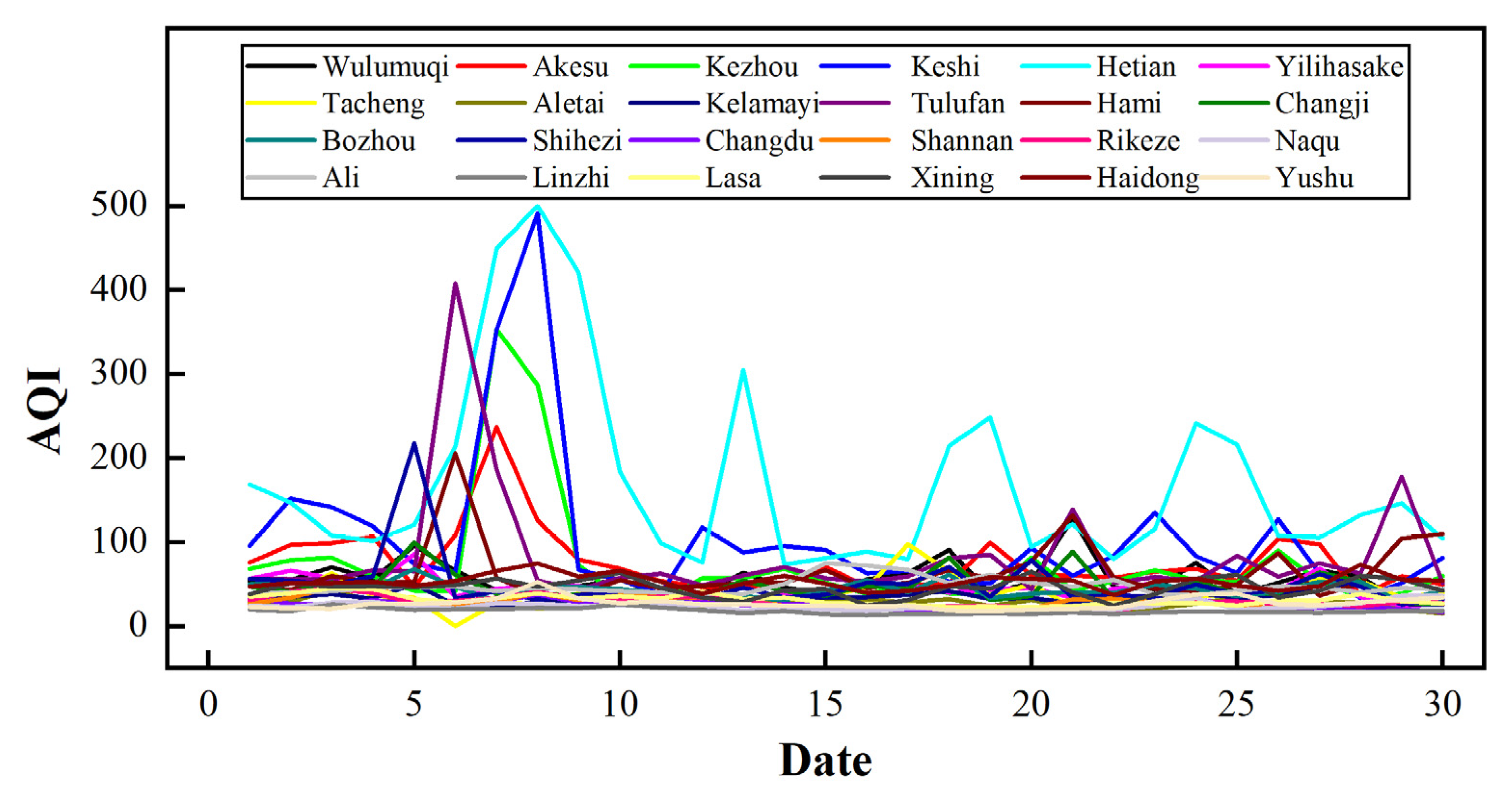
4.2. Hourly PM_2.5 and PM₁₀ Concentrations in China

AOD, RH, BLH, and other auxiliary data and calculation methods used by the two pollutants are similar, while the ground monitoring data are different. The calculation of PM is highly dependent on the coverage of the AOD and its temporal and spatial resolution. Thus, for PM_2.5 and PM₁₀ estimation, hourly and 1 km resolution can be achieved.

Figure 5 and Figure 6 show the spatial distribution of model-estimated mean PM_2.5 and PM₁₀ concentrations in China at different times of the day at 5–6 and 9–10 June 2020, respectively. For most of the study areas, the PM_2.5 concentrations are below 90 μg/m³. Additionally, the PM₁₀ concentrations are below 100 μg/m³. The lowest average PM_2.5 concentrations is recorded at 15:00 p.m. (LST), and the highest at 09:00 a.m. (LST). The lowest mean PM₁₀ concentration was at 15:00 p.m. (LST), and the highest was at 09:00 a.m. (LST). This is similar to but not entirely consistent with previous studies [25,37]. Before sunrise, the height of the atmospheric boundary layer is relatively low, and aerosols are concentrated in the lower layers of the atmosphere. This results in relatively high PM_2.5 concentrations near the ground. The atmosphere is then heated with increasing radiation from the height of the sun, leading to expansion and thermodynamic uplift, with a corresponding rise in the boundary layer [43,44]. As a result, fine particulates in the atmosphere also move into the upper atmosphere, leading to a gradual decrease in PM_2.5 concentrations at ground level. This is due to the short time series used in this study, which is insufficient to form a more obvious statistical pattern. The variation in PM does not follow the same clear daily cycle as the BLH, because the relationship between PM concentrations and PBL varies considerably with geographical location, season, and other meteorological conditions [45].

Figure 7 and Figure 8 show the daily daytime averages of PM_2.5 mass concentration and PM₁₀ mass concentration for each day and the corresponding station data, respectively. The first column in each figure shows the data estimated by the model, and the second column shows the station mean data (columns 1 and 2, from left to right). The station averages are the mean of the hourly measurements from 08:00 to 17:00 each day, where unusable data were excluded. The model-estimated PM concentrations are generally consistent with the spatial and temporal distribution of PM concentrations observed at ground level. Spatially, the higher PM_2.5 pollution concentrations are found in central China, including Shaanxi, Shanxi, Henan, and Shandong, similar to previous studies [25]. However, higher pollution was observed in Xinjiang and the Tibetan–Qinghai Plateau, which is more exceptional in June 2020. Figure 9 shows the AQI change graphs for selected cities in Tibet, Xinjiang, and Qinghai in June 2020. AQI (air quality index) describes how clean or polluted the air is, with associated health effects. The AQI is calculated by the Chinese Environmental Protection Bureau based on air quality evaluation standards by monitoring sulphur dioxide, nitrogen dioxide, PM₁₀, PM_2.5, carbon monoxide, and ozone. AQI enables air quality to be presented in a uniform evaluation standard [46]. Currently, the main influences on AQI are PM_2.5 and PM₁₀. The specificity of the air quality in these regions from 5 to 10 June 2020 can be seen. Unfortunately, the raw data for the 7th and 8th are missing due to the cloud, so we have chosen 5–6 and 9–10 June 2020 for the study. The Tibetan–Qinghai Plateau and the area around the Tian Shan Mountains are clean areas with little anthropogenic pollution, and the main source of PM is soil dust. Therefore, the high concentration levels reported during the study time are due to natural causes. In central and eastern China, where air pollution is relatively high, a decreasing gradient from north to south can be seen, consistent with previous studies (e.g., [47,48,49]).

The analysis in this section shows that the model is sensitive to the estimates of the ground-level hourly PM_2.5 and PM₁₀ concentrations. Additionally, it can predict the following pollution trends.

5. Discussion

5.1. Comparison with Previous Studies

The relationship between AOD and PM_2.5 concentration is known to be more complex due to the influence of multiple factors (e.g., aerosol type, meteorological variables). IGTWR is a traditional data analysis method that provides a more straightforward representation of the relationship between PM and various variables than the emerging machine learning approach. Moreover, compared to machine learning, IGTWR is less prone to overfitting. The present study improves the quality of the model by defining the generalised distance with NDVI. Additionally, it employs the improved model to estimate hourly PM_2.5 and PM₁₀ concentrations in China. The research conducted by Xu et al. showed that the quality of the model to estimate PM_2.5 could be improved by introducing NDVI into the regression model [34]. The CV of the IGTWR model employed in the present study indicated that the model showed an excellent estimation ability of PM_2.5 and PM₁₀ concentrations. This advantage is reflected in statistical indicators. Specifically, the R² was 0.909 and 0.915, and the RMSE was 5.802 µg/m³ and 12.939 µg/m³ for PM_2.5 and PM₁₀, respectively. In this regard, the model employed in the present study was superior to previous models, in which FY-4A AOD data were used to estimated PM_2.5 concentration. Jiang et al. [35] estimated PM_2.5 concentrations using physical methods and FY-4A AOD with a maximum R² of 0.39, but the values were still over-or underestimated. Mao et al. [8] used the random forest algorithm and FY-4A AOD for the estimation of PM_2.5 in China. Additionally, they found that the use of the FY-4A improved 17% spatial coverage compared to the Himawari-8-based PM_2.5 retrievals. In addition to the satisfying performance and advantages of the method employed in the present study, the model developed for estimating hourly PM concentrations can provide detailed information on the daily cycle of PM concentrations at a good spatial resolution, which can help us to facilitate an in-depth study of PM_2.5.

5.2. Potential Limitations and Room for Model Improvement

Although this model can predict PM_2.5 and PM₁₀ concentrations well, there are still several potential limitations, and there is scope for future improvements. Reanalysis data are commonly used in most studies due to the lack of high spatial and temporal resolution PBLH and RH observations. The raw resolution of the PBLH and RH product is only 0.25° × 0.25°, which may affect the estimation accuracy of hourly PM concentrations. Liu et al. believed that model performance would be improved if high-frequency meteorological data were available [50]. Moreover, Gui et al. constructed a virtual ground-based PM_2.5 observation network by using an extreme gradient boosting (XGBoost) model with high-density meteorological observations as the main predictor. Additionally, results showed that this network had great potential for reconstructing historical PM_2.5 concentrations [50]. This is a significant improvement to the application of the model employed in the present study to historical situations.

The present model is limited by the missing AOD and the necessity to use PM measurements. More specifically, PM concentrations cannot be estimated in the missing AOD fraction. Yin et al. proposed a method to estimate PM_2.5 distribution with the Himawari-8 top-of-atmosphere reflectance (TOAR) over China, effectively estimating PM_2.5 in areas where valid AOD observations are not available. The spatial and temporal coverage of PM_2.5 estimated by TOAR is approximately four times higher than that based on AOD data [51]. Park et al. also developed an estimation model for spatially continuous AOD and PM that can be used for all-sky conditions [5]. All these studies have significant implications for the improvement of the present model.

6. Conclusions

In this study, the IGTWR model is employed as the basis for model improvement by adding NDVI data to change the definition of the generalised distance. The mass concentrations of PM_2.5 and PM₁₀ are estimated using FY-4A data with other ancillary data. The results show that FY-4 combined with IGTWR model to estimate PM_2.5 and PM₁₀ concentrations in China accurately. From the cross-validation results, it appears that the estimation effect of this model on PM_2.5 is better than that on PM₁₀. Further research will investigate this and improve the model to adapt it to PM₁₀ estimation.

The PM mass concentrations estimated throughout the study were validated against measurements from ground stations and compared qualitatively with the results of the model before the improvement. The PM_2.5 and PM₁₀ estimates were in good agreement with ground station measurements, with correlation coefficients of 0.909 and 0.915, respectively. The predicted and measured values of PM_2.5 and PM₁₀ concentrations are consistent across the study area.

Unlike the models used in previous studies, the IGTWR model redefines distance in a broad sense using land use classifications. Hu et al. [52] used spatial distance as a weighting parameter; later, Huang et al. [41] extended this distance to geographic and temporal distances by introducing days into the model. The IGTWR model is used for this study. Date, hour, and NDVI are used to construct the generalised distances. Compared to the previous study by Xue et al. [36] the model effect is reduced by extending the area from central and eastern China to the whole country, adding areas with sparser ground stations. As shown in Figure 7 and Figure 8, the small area covered by the AOD is due to the absence of the bright surface area itself and cloud cover. The AOD data cover fewer ground stations, resulting in a training sample of just over 6000 points. One of the reasons for the overfitting is the sparse number of sample points, so the tenfold cross-validation result is worse than the model fitting result. The ability of the model to predict particulate matter has been reduced, but the overall picture remains within acceptable limits. This is due to the characteristics of the GWR model.

Future research must address several issues. Firstly, fixed bandwidth is used in this model, but it is unstable. Subsequent studies may try to use dynamic bandwidth to improve its stability. Secondly, the reason for the weaker prediction of PM is the lack of sample points. As the duration of the study increases with the quality of the FY-4A data, it can be expected that this method is able to estimate ground-level PM concentrations with higher confidence at seasonal levels or higher temporal resolutions. Thirdly, the redefinition of the generalised distance is the key point for improving the GWR in Equation (7). Therefore, the use of other types of data to improve the definition of generalised distances (e.g., DEM, etc.) and to make use of the data provided by FY-4A will be an interesting topic for future research. Finally, the FY-4A data and the model can be applied in the future together with the enhanced dust intensity index (EDII) [53] for the detection of dust areas, dust detection, and intensity estimation.

References

1. Tao, J.; Gao, J.; Zhang, L.; Zhang, R.; Che, H.; Zhang, Z.; Lin, Z.; Jing, J.; Cao, J.; Hsu, S.C. PM2.5 pollution in a megacity of southwest China: Source apportionment and implication. Atmos. Chem. Phys. 2014, 14, 8679–8699. [Google Scholar] [CrossRef] [Green Version]
2. Cohen, A.J.; Brauer, M.; Burnett, R. Estimates and 25-year trends of the global burden of disease attributable to ambient air pollution: An analysis of data from the Global Burden of Diseases Study 2015 (vol 389, pg 1907, 2017). Lancet 2018, 391, 1576. [Google Scholar] [CrossRef] [Green Version]
3. Wang, J.; Christopher, S.A. Intercomparison between satellite-derived aerosol optical thickness and PM2.5 mass: Implications for air quality studies. Geophys. Res. Lett. 2003, 30, 510–528. [Google Scholar] [CrossRef]
4. Shaw, N.; Gorai, A.K. Study of aerosol optical depth using satellite data (MODIS Aqua) over Indian Territory and its relation to particulate matter concentration. Environ. Dev. Sustain. 2020, 22, 265–279. [Google Scholar] [CrossRef]
5. Park, S.; Lee, J.; Im, J.; Song, C.-K.; Choi, M.; Kim, J.; Lee, S.; Park, R.; Kim, S.-M.; Yoon, J.; et al. Estimation of spatially continuous daytime particulate matter concentrations under all sky conditions through the synergistic use of satellite-based AOD and numerical models. Sci. Total Environ. 2020, 713, 136516. [Google Scholar] [CrossRef] [PubMed]
6. Wei, J.; Li, Z.Q.; Cribb, M.; Huang, W.; Xue, W.H.; Sun, L.; Guo, J.P.; Peng, Y.R.; Li, J.; Lyapustin, A.; et al. Improved 1 km resolution PM2.5 estimates across China using enhanced space-time extremely randomized trees. Atmos. Chem. Phys. 2020, 20, 3273–3289. [Google Scholar] [CrossRef] [Green Version]
7. She, L.; Xue, Y.; Yang, X.; Leys, J.; Guang, J.; Che, Y.; Fan, C.; Xie, Y.; Li, Y. Joint Retrieval of Aerosol Optical Depth and Surface Reflectance Over Land Using Geostationary Satellite Data. IEEE Trans. Geosci. Remote Sens. 2019, 57, 1489–1501. [Google Scholar] [CrossRef]
8. Mao, F.; Hong, J.; Min, Q.; Gong, W.; Zang, L.; Yin, J. Estimating hourly full-coverage PM2.5 over China based on TOA reflectance data from the Fengyun-4A satellite. Environ. Pollut. 2021, 270, 116119. [Google Scholar] [CrossRef]
9. Liu, Y.; Park, R.J.; Jacob, D.J.; Li, Q.B.; Kilaru, V.; Sarnat, J.A. Mapping annual mean ground-level PM2.5 concentrations using Multiangle Imaging Spectroradiometer aerosol optical thickness over the contiguous United States. J. Geophys. Res.-Atmos. 2004, 109, 10. [Google Scholar] [CrossRef]
10. Chu, D.A.; Tsai, T.-C.; Chen, J.-P.; Chang, S.-C.; Jeng, Y.-J.; Chiang, W.-L.; Lin, N.-H. Interpreting aerosol lidar profiles to better estimate surface PM2.5 for columnar AOD measurements. Atmos. Environ. 2013, 79, 172–187. [Google Scholar] [CrossRef]
11. Zhang, Y.; Li, Z. Remote sensing of atmospheric fine particulate matter (PM2.5) mass concentration near the ground from satellite observation. Remote Sens. Environ. 2015, 160, 252–262. [Google Scholar] [CrossRef]
12. You, W.; Zang, Z.; Zhang, L.; Zhang, M.; Pan, X.; Li, Y. A nonlinear model for estimating ground-level PM10 concentration in Xi’an using MODIS aerosol optical depth retrieval. Atmos. Res. 2016, 168, 169–179. [Google Scholar] [CrossRef]
13. Nordio, F.; Kloog, I.; Coull, B.A.; Chudnovsky, A.; Grillo, P.; Bertazzi, P.A.; Baccarelli, A.A.; Schwartz, J. Estimating spatio-temporal resolved PM10 aerosol mass concentrations using MODIS satellite data and land use regression over Lombardy, Italy. Atmos. Environ. 2013, 74, 227–236. [Google Scholar] [CrossRef]
14. Park, S.; Shin, M.; Im, J.; Song, C.-K.; Choi, M.; Kim, J.; Lee, S.; Park, R.; Kim, J.; Lee, D.-W.; et al. Estimation of ground-level particulate matter concentrations through the synergistic use of satellite observations and process-based models over South Korea. Atmos. Chem. Phys. 2019, 19, 1097–1113. [Google Scholar] [CrossRef] [Green Version]
15. Hou, W.; Li, Z.; Zhang, Y.; Xu, H.; Zhang, Y.; Li, K.; Li, D.; Wei, P.; Ma, Y. Using support vector regression to predict PM10 and PM2.5. In 35th International Symposium on Remote Sensing of Environment; Guo, H., Ed.; IOP Conference Series-Earth and Environmental Science: Bristol, UK, 2014; Volume 17. [Google Scholar]
16. Jiang, T.T.; Chen, B.; Nie, Z.; Ren, Z.H.; Xu, B.; Tang, S.H. Estimation of hourly full-coverage PM2.5 concentrations at 1-km resolution in China using a two-stage random forest model. Atmos. Res. 2021, 248, 105146. [Google Scholar] [CrossRef]
17. Chen, W.; Ran, H.; Cao, X.; Wang, J.; Teng, D.; Chen, J.; Zheng, X. Estimating PM2.5 with high-resolution 1-km AOD data and an improved machine learning model over Shenzhen, China. Sci. Total Environ. 2020, 746, 141093. [Google Scholar] [CrossRef]
18. Wei, J.; Huang, W.; Li, Z.; Xue, W.; Peng, Y.; Sun, L.; Cribb, M. Estimating 1-km-resolution PM2.5 concentrations across China using the space-time random forest approach. Remote Sens. Environ. 2019, 231, 111221. [Google Scholar] [CrossRef]
19. Shin, M.; Kang, Y.; Park, S.; Im, J.; Yoo, C.; Quackenbush, L.J. Estimating ground-level particulate matter concentrations using satellite-based data: A review. Gisci. Remote Sens. 2020, 57, 174–189. [Google Scholar] [CrossRef]
20. Friedman, J.H. Greedy function approximation: A gradient boosting machine. Ann. Stat. 2001, 29, 1189–1232. [Google Scholar] [CrossRef]
21. Chen, T.Q.; Guestrin, C.; Assoc Comp, M. XGBoost: A Scalable Tree Boosting System. In Proceedings of the 22nd acm sigkdd international conference on knowledge discovery and data mining 2016, San Francisco, CA, USA, 13–17 August 2016; pp. 785–794. [Google Scholar]
22. Ma, Z.; Hu, X.; Huang, L.; Bi, J.; Liu, Y. Estimating Ground-Level PM2.5 in China Using Satellite Remote Sensing. Environ. Sci. Technol. 2014, 48, 7436–7444. [Google Scholar] [CrossRef]
23. Bai, Y.; Wu, L.; Qin, K.; Zhang, Y.; Shen, Y.; Zhou, Y. A Geographically and Temporally Weighted Regression Model for Ground-Level PM2.5 Estimation from Satellite-Derived 500 m Resolution AOD. Remote Sens. 2016, 8, 262. [Google Scholar] [CrossRef] [Green Version]
24. Guo, Y.; Tang, Q.; Gong, D.-Y.; Zhang, Z. Estimating ground-level PM2.5 concentrations in Beijing using a satellite-based geographically and temporally weighted regression model. Remote Sens. Environ. 2017, 198, 140–149. [Google Scholar] [CrossRef]
25. You, W.; Zang, Z.; Zhang, L.; Li, Y.; Pan, X.; Wang, W. National-Scale Estimates of Ground-Level PM2.5 Concentration in China Using Geographically Weighted Regression Based on 3 km Resolution MODIS AOD. Remote Sens. 2016, 8, 184. [Google Scholar] [CrossRef] [Green Version]
26. Wei, J.; Li, Z.; Xue, W.; Sun, L.; Fan, T.; Liu, L.; Su, T.; Cribb, M. The ChinaHighPM(10) dataset: Generation, validation, and spatiotemporal variations from 2015 to 2019 across China. Environ. Int. 2021, 146, 106290. [Google Scholar] [CrossRef]
27. Yang, Q.; Yuan, Q.; Yue, L.; Li, T.; Shen, H.; Zhang, L. The relationships between PM2.5 and aerosol optical depth (AOD) in mainland China: About and behind the spatio-temporal variations. Environ. Pollut. 2019, 248, 526–535. [Google Scholar] [CrossRef]
28. Xu, Q.; Chen, X.; Yang, S.; Tang, L.; Dong, J. Spatiotemporal relationship between Himawari-8 hourly columnar aerosol optical depth (AOD) and ground-level PM2.5 mass concentration in mainland China. Sci. Total Environ. 2021, 765, 144241. [Google Scholar] [CrossRef]
29. Wang, J.; Li, Z. Estimation of ground-level dry PM2.5concentrations at 3 km resolution over Beijing using Geostationary Ocean Colour Imager. Remote Sens. Lett. 2020, 11, 913–922. [Google Scholar] [CrossRef]
30. Wang, X.; Wang, F.; Jia, L.; Su, H.; Lin, M. IEEE Estimating PM2.5 concentrations of high-resolution in taiwan island using gf-1 wfv data. In Proceedings of the IEEE International Geoscience and Remote Sensing Symposium (IGARSS), Yokohama, Japan, 28 July–2 August 2019; pp. 7846–7849. [Google Scholar]
31. Zhao, C.; Wang, Q.; Ban, J.; Liu, Z.; Zhang, Y.; Ma, R.; Li, S.; Li, T. Estimating the daily PM2.5 concentration in the Beijing-Tianjin-Hebei region using a random forest model with a 0.01 degrees x 0.01 degrees spatial resolution. Environ. Int. 2020, 134, 105297. [Google Scholar] [CrossRef]
32. Yang, S.H.; Jeong, J.I.; Park, R.J.; Kim, M.J. Impact of Meteorological Changes on Particulate Matter and Aerosol Optical Depth in Seoul during the Months of June over Recent Decades. Atmosphere 2020, 11, 1282. [Google Scholar] [CrossRef]
33. Li, R.; Mei, X.; Chen, L.; Wang, Z.; Jing, Y.; Wei, L. Influence of Spatial Resolution and Retrieval Frequency on Applicability of Satellite-Predicted PM2.5 in Northern China. Remote Sens. 2020, 12, 736. [Google Scholar] [CrossRef] [Green Version]
34. Xu, X.; Zhang, C. Estimation of ground-level PM2.5concentration using MODIS AOD and corrected regression model over Beijing, China. PLoS ONE 2020, 15, e0240430. [Google Scholar] [CrossRef]
35. Jiang, Q.; Gui, H.; Zhang, T.; Wang, F.; Zhang, B.; Chi, X.; Xu, R. FY-4A satellite data based on grid surface atmospheric particulate concentration estimation in China. Weather 2020, 46, 1297–1309. [Google Scholar]
36. Xue, Y.; Li, Y.; Guang, J.; Tugui, A.; She, L.; Qin, K.; Fan, C.; Che, Y.; Xie, Y.; Wen, Y.; et al. Hourly PM2.5 Estimation over Central and Eastern China Based on Himawari-8 Data. Remote Sens. 2020, 12, 855. [Google Scholar] [CrossRef] [Green Version]
37. Xu, X.; Liu, J.; Zhuang, D. Remote sensing Monitoring methods of land use/cover changes in national scale. Anhui Agric. Sci. 2012, 40, 2365–2369. [Google Scholar]
38. Yang, J.; Zhang, Z.Q.; Wei, C.Y.; Lu, F.; Guo, Q. Introducing the New Generation of Chinese Geostationary Weather Satellites, Fengyun-4. Bull. Am. Meteorol. Soc. 2017, 98, 1637–1658. [Google Scholar] [CrossRef]
39. Xia, X.; Min, J.; Shen, F.; Wang, Y.; Xu, D.; Yang, C.; Zhang, P. Aerosol data assimilation using data from Fengyun-4A, a next-generation geostationary meteorological satellite. Atmos. Environ. 2020, 237, 117695. [Google Scholar] [CrossRef]
40. Miao, Y.; Liu, S.; Guo, J.; Huang, S.; Yan, Y.; Lou, M. Unraveling the relationships between boundary layer height and PM2.5 pollution in China based on four-year radiosonde measurements. Environ. Pollut. 2018, 243, 1186–1195. [Google Scholar] [CrossRef]
41. Huang, B.; Wu, B.; Barry, M. Geographically and temporally weighted regression for modeling spatio-temporal variation in house prices. Int. J. Geogr. Inf. Sci. 2010, 24, 383–401. [Google Scholar] [CrossRef]
42. Diego Rodriguez, J.; Perez, A.; Antonio Lozano, J. Sensitivity Analysis of k-Fold Cross Validation in Prediction Error Estimation. IEEE Trans. Pattern Anal. Mach. Intell. 2010, 32, 569–575. [Google Scholar] [CrossRef] [PubMed]
43. Guo, J.; Miao, Y.; Zhang, Y.; Liu, H.; Li, Z.; Zhang, W.; He, J.; Lou, M.; Yan, Y.; Bian, L.; et al. The climatology of planetary boundary layer height in China derived from radiosonde and reanalysis data. Atmos. Chem. Phys. 2016, 16, 13309–13319. [Google Scholar] [CrossRef] [Green Version]
44. Wang, L.; Gong, W.; Xia, X.; Zhu, J.; Li, J.; Zhu, Z. Long-term observations of aerosol optical properties at Wuhan, an urban site in Central China. Atmos. Environ. 2015, 101, 94–102. [Google Scholar] [CrossRef]
45. Su, T.; Li, Z.; Kahn, R. Relationships between the planetary boundary layer height and surface pollutants derived from lidar observations over China: Regional pattern and influencing factors. Atmos. Chem. Phys. 2018, 18, 15921–15935. [Google Scholar] [CrossRef] [Green Version]
46. Technical Regulation on Ambient Air Quality Index (on Trial): HJ, 633–2012; China Environmental Science Press: Beijing, China, 2012.
47. Ma, Z.; Hu, X.; Sayer, A.M.; Levy, R.; Zhang, Q.; Xue, Y.; Tong, S.; Bi, J.; Huang, L.; Liu, Y. Satellite-Based Spatiotemporal Trends in PM2.5 Concentrations: China, 2004–2013. Environ. Health Perspect. 2016, 124, 184–192. [Google Scholar] [CrossRef] [Green Version]
48. Li, T.; Shen, H.; Yuan, Q.; Zhang, X.; Zhang, L. Estimating Ground-Level PM2.5 by Fusing Satellite and Station Observations: A Geo-Intelligent Deep Learning Approach. Geophys. Res. Lett. 2017, 44, 11985–11993. [Google Scholar] [CrossRef] [Green Version]
49. Liu, J.; Weng, F.; Li, Z.; Cribb, M.C. Hourly PM2.5 Estimates from a Geostationary Satellite Based on an Ensemble Learning Algorithm and Their Spatiotemporal Patterns over Central East China. Remote Sens. 2019, 11, 2120. [Google Scholar] [CrossRef] [Green Version]
50. Gui, K.; Che, H.; Zeng, Z.; Wang, Y.; Zhai, S.; Wang, Z.; Luo, M.; Zhang, L.; Liao, T.; Zhao, H.; et al. Construction of a virtual PM2.5 observation network in China based on high-density surface meteorological observations using the Extreme Gradient Boosting model. Environ. Int. 2020, 141, 105801. [Google Scholar] [CrossRef]
51. Yin, J.; Mao, F.; Zang, L.; Chen, J.; Lu, X.; Hong, J. Retrieving PM2.5 with high spatio-temporal coverage by TOA reflectance of Himawari-8. Atmos. Pollut. Res. 2021, 12, 14–20. [Google Scholar] [CrossRef]
52. Hu, X.; Waller, L.A.; Al-Hamdan, M.Z.; Crosson, W.L.; Estes, M.G., Jr.; Estes, S.M.; Quattrochi, D.A.; Sarnat, J.A.; Liu, Y. Estimating ground-level PM2.5 concentrations in the southeastern US using geographically weighted regression. Environ. Res. 2013, 121, 1–10. [Google Scholar] [CrossRef] [PubMed]
53. She, L.; Xue, Y.; Yang, X.; Guang, J.; Li, Y.; Che, Y.; Fan, C.; Xie, Y. Dust Detection and Intensity Estimation Using Himawari-8/AHI Observation. Remote Sens. 2018, 10, 490. [Google Scholar] [CrossRef] [Green Version]
Figure 1. The distribution of land use types over China in 2020 [37]. The number of different land use types refers to the land use and cover change (LUCC) classification system, as shown in Table 1. The black boundary line represents the study area.
Remotesensing 13 04276 g001
Figure 2. Scatter plots for (a) model fitting result and (b) tenfold cross-validation results for PM2.5. Scatter plots for (c) model fitting result and (d) tenfold cross-validation results for PM10. The colour represents the sample density.
Remotesensing 13 04276 g002aRemotesensing 13 04276 g002b
Figure 3. Scatter plots for (a) model fitting result and (b) tenfold cross-validation results for PM2.5. Scatter plots for (c) model fitting result and (d) tenfold cross-validation results for PM10. The colour represents the sample density. This part is calculated using land use data instead of NDVI.
Remotesensing 13 04276 g003
Figure 4. The measured and estimated PM2.5/PM10 ratios.
Remotesensing 13 04276 g004
Figure 5. Average hourly PM2.5 concentration in 5–6 and 9–10 June 2020, 8:00–17:00 (LST), from (a) to (j).
Remotesensing 13 04276 g005aRemotesensing 13 04276 g005b
Figure 6. Average hourly PM10 concentration on 5–6 and 9–10 June 2020, 8:00–17:00 (LST), from (a) to (j).
Remotesensing 13 04276 g006aRemotesensing 13 04276 g006bRemotesensing 13 04276 g006c
Figure 7. Average daily PM2.5 concentration on 5–6 and 9–10 June 2020. Column 1 from (a) to (d) is model estimates and column 2 from (e) to (h) is station observations (columns 1 and 2, from left to right).
Remotesensing 13 04276 g007aRemotesensing 13 04276 g007b
Figure 8. Average daily PM10 concentration on 5–6 and 9–10 June 2020. Column 1 from (a) to (d) is model estimates and column 2 from (e) to (h) is station observations (columns 1 and 2, from left to right).
Remotesensing 13 04276 g008aRemotesensing 13 04276 g008b
Figure 9. Average daily AQI for selected cities in western China in June 2020.
Remotesensing 13 04276 g009