MIMO-SAR Interferometric Measurements for Structural Monitoring: Accuracy and Limitations

Abstract

Terrestrial Radar Interferometry (TRI) is a measurement technique capable of measuring displacements with high temporal resolution at high accuracy. Current implementations of TRI use large and/or movable antennas for generating two-dimensional displacement maps. Multiple Input Multiple Output Synthetic Aperture Radar (MIMO-SAR) systems are an emerging alternative. As they have no moving parts, they are more easily deployable and cost-effective. These features suggest the potential usage of MIMO-SAR interferometry for structural health monitoring (SHM) supplementing classical geodetic and mechanical measurement systems. The effects impacting the performance of MIMO-SAR systems are, however, not yet sufficiently well understood for practical applications. In this paper, we present an experimental investigation of a MIMO-SAR system originally devised for automotive sensing, and assess its capabilities for deformation monitoring. The acquisitions generated for these investigations feature a 180${}^{\circ }$ Field-of-View (FOV), distances of up to 60 m and a temporal sampling rate of up to 400 Hz. Experiments include static and dynamic setups carried out in a lab-environment and under more challenging meteorological conditions featuring sunshine, fog, and cloud-cover. The experiments highlight the capabilities and limitations of the radar, while allowing quantification of the measurement uncertainties, whose sources and impacts we discuss. We demonstrate that, under sufficiently stable meteorological conditions with humidity variations smaller than 1%, displacements as low as 25 μm can be detected reliably. Detecting displacements occurring over longer time frames is limited by the uncertainty induced by changes in the refractive index.

1. Introduction

Radar interferometry is used in a wide variety of monitoring applications ranging from small-scale phenomena like landslides to assessing large mass-movements as occurring e.g., after earthquakes [1,2,3,4]. Measurements are extracted from the relative attenuation, delay, and frequency shift of signals radiated by a transmitting antenna (TXA), reflected by an object, and detected by the receiving antenna (RXA). Radar interferometry specifically uses the phase information of the complex received signal to derive metric displacements in line-of-sight (LOS), see Section 2.4 for more details.

The field-of-view (FOV) and angular resolution of radar systems depend on the size of the transmitting antenna and the wavelength of the radio wave, see Section 2.2 and Section 2.3. Achieving a large FOV and a high angular resolution requires either large rotating antennas (real aperture radar, RAR) or small antennas radiating and receiving from different positions (synthetic aperture radar, SAR). Radar sensors can be mounted on spaceborne, airborne, or ground-based platforms. The latter, in the form of terrestrial radar interferometry (TRI), is becoming increasingly attractive for smaller scale monitoring tasks leveraging its high spatiotemporal resolution and capability for highly precise deformation measurements. TRI is applied for measuring surface changes in geomonitoring, structural monitoring, and glacier and snow monitoring [5,6]. Those radar systems operate on the C-, X-, and Ku-bands, with corresponding wavelengths of 5.0, 3.1, and 1.7 cm respectively. They can achieve deformation accuracy in the sub-millimeter ranges.

Current high-resolution ground-based RAR and SAR systems used for monitoring rely on moving parts making them expensive and complex to maintain. The autonomous driving industry pushed the development of MIMO-SAR, short for multiple input multiple output synthetic aperture radar, as an alternative to SAR with reduced mechanical complexity (i.e., no moving parts). Despite reduced hardware cost and size, MIMO-SAR provides high angular and range resolution [7], and it can acquire measurements of the entire area within the FOV within a fraction of a second and under adverse weather conditions. These characteristics suggest deploying MIMO-SAR for structural health monitoring (SHM).

MIMO-SAR in Structural Health Monitoring

The goal of SHM is the early detection of areas of structural weakness in engineering structures. SHM systems consists of multiple interacting components. Data acquisition is carried out by sensors, which may be installed in-situ like optical fibers [8], piezoelectric sensors [9], GNSS (Global Navigation Satellite Systems) receivers [10], accelerometers [11], and inclinometers [12]. Alternatively, the sensors might gather information relevant to assessing structural soundness remotely as is the case with robotic total stations [13], 3D-laser scanners [14], or radar systems [15,16,17,18]. Subsequently experts interpret the observations, diagnose the health status of the structure, and initiate on-site inspection of maintenance work in case of irregularities.

Vibrations form a key diagnostic in SHM [19]. If these fast deformations can be measured, a comparison to the expected behavior of an uncompromised structure allows detecting flaws and weaknesses. Many common structures like bridges and buildings vibrate with a natural frequency of 10 Hz or below [20] with some reaching up to 50 Hz [21]. The amplitudes of vertical displacements are usually in the range of sub-millimeters reaching up to a couple of decimeters with a maximum velocity of about 2.5 cm/s [22] for highly flexible structures such as footbridges. According to the Shannon-Nyquist theorem [23] on baseband signals, a sensor used for vibration monitoring needs to sample with a temporal frequency at least twice as high as the highest frequency of the deformation signal to guarantee a complete reconstruction and avoid aliasing due to undersampling.

Commercial MIMO-SAR systems suitable for SHM are rare and most systems are in-house developments.

Table 1. MIMO-SAR systems for SHM.

System Name or First Publication	Year	Angular Res. [°]	Range Res. [m]	Acquisition Rate [Hz]	Accuracy Def. [µm]	Reference
TI AWR1642	2019	14.3	4	16.7	-	[24]
ScanBrick	2019	few deg.	>5	<1000	10	[25]
Pieraccini et al.	2019	2.865	47	1/30	100	[26,27]
Hu et al.	2017	0.466	37.5	37	sub-mm	[28,29,30,31]
Melissa	2013	1.2	89	1.4	10	[32,33]

provides an overview of MIMO-SAR systems whose characteristics and deployment for SHM projects have been publicized in scientific journals or openly accessible media.

Already in 2013, Tarchi et al. [32] developed a MIMO-SAR system called Melissa, which operated in the Ku-band and featured 12 TXA and 12 RXA. They used it to monitor the movements of the cruise ship Costa Concordia after its sinking and concluded that MIMO-SAR systems can be operated by day and night, are robust against environmental conditions, operate remotely without requiring the installation of reference targets, and provide a large number of 2D displacement observations [33]. Like with all radar systems, phase unwrapping errors occured when the object moved more than $\lambda /4$ between consecutive acquisitions (i.e., >7 mm/s, considering specific wavelength and acquisition rate). Hu et al. [28] developed another Ku-band MIMO-SAR system with 16 TXA and up to 32 RXA. They compared vibration frequencies and amplitudes derived from MIMO-SAR observations to the ones generated by a vibration calibrator and found the frequencies to be consistent and the amplitudes underestimated by 5 to 10% [31]. In the same paper, their system is applied to measure the vibrations of a car with running engine and a train bridge with and without train traffic. They were able to distinguish vibrations of different vibrating objects within the monitored area. Pieraccini et al. [26] developed an X-band MIMO-SAR system with 4 TXA and 4 RXA and measured the deformation of a pedestrian bridge loaded by a car at different positions. While measuring a corner cube mounted below a car bridge [27], a subsequent comparison with a static Ku-band RAR system revealed a disadvantage in sampling time but an advantage in azimuthal resolution. D’Aria et al. [25] used ScanBrick, which is —to the knowledge of the authors —the first commercially available MIMO-SAR system specifically advertised for infrastructures and geophysical applications. They observed a church facade subjected to construction work and a train bridge with a passing train. They were able to detect deformations in the sub-mm to mm range but had no independent reference measurements for comparison. Gambi et al. [24] evaluated an automotive radar with 2 TXA and 4 RXA and measured the displacements of a traffic bridge concluding that W-band radar instruments would be able to measure vibrations.

The research so far shows the potential for MIMO-SAR to enable monitoring of highly dynamical phenomena as demonstrated on actual application cases. However, the effects determining the reliability of MIMO-SAR observations are still not completely understood. In this paper, we contribute to this understanding by providing a more formal assessment of achievable performance of an automotive MIMO-SAR system by comparison with highly accurate reference measurements and measurements under stable indoor conditions and in an outdoor situation.

We identify three key criteria for the assessment: (1) the range of measurable and robustly detectable displacements; (2) the range of acquisition frequencies and their relationship to typical oscillation frequencies of engineering structures; (3) the influence of environmental conditions (e.g., humidity, temperature) on measurements. To this end, we explain the concept and principles of MIMO-SAR measurements (Section 2) upon which we describe three experimental setups (Section 3) designed to isolate the main effects impacting the reliability of such measurements. The results of these experiments are presented and interpreted in Section 4, and we summarize our investigation with concluding remarks regarding MIMO-SAR’s precision and give an outlook of further steps in Section 5.

2. MIMO-SAR Principles

The basis of MIMO-SAR measurements are covered in this section, describing the antenna configuration (Section 2.1) and its influence on the field-of-view (Section 2.2), as well as the azimuth resolution (Section 2.3). These descriptions are followed by an analysis of the range resolution capabilities (Section 2.3) and general remarks on the measurement principle underlying radar interferometry (Section 2.4).

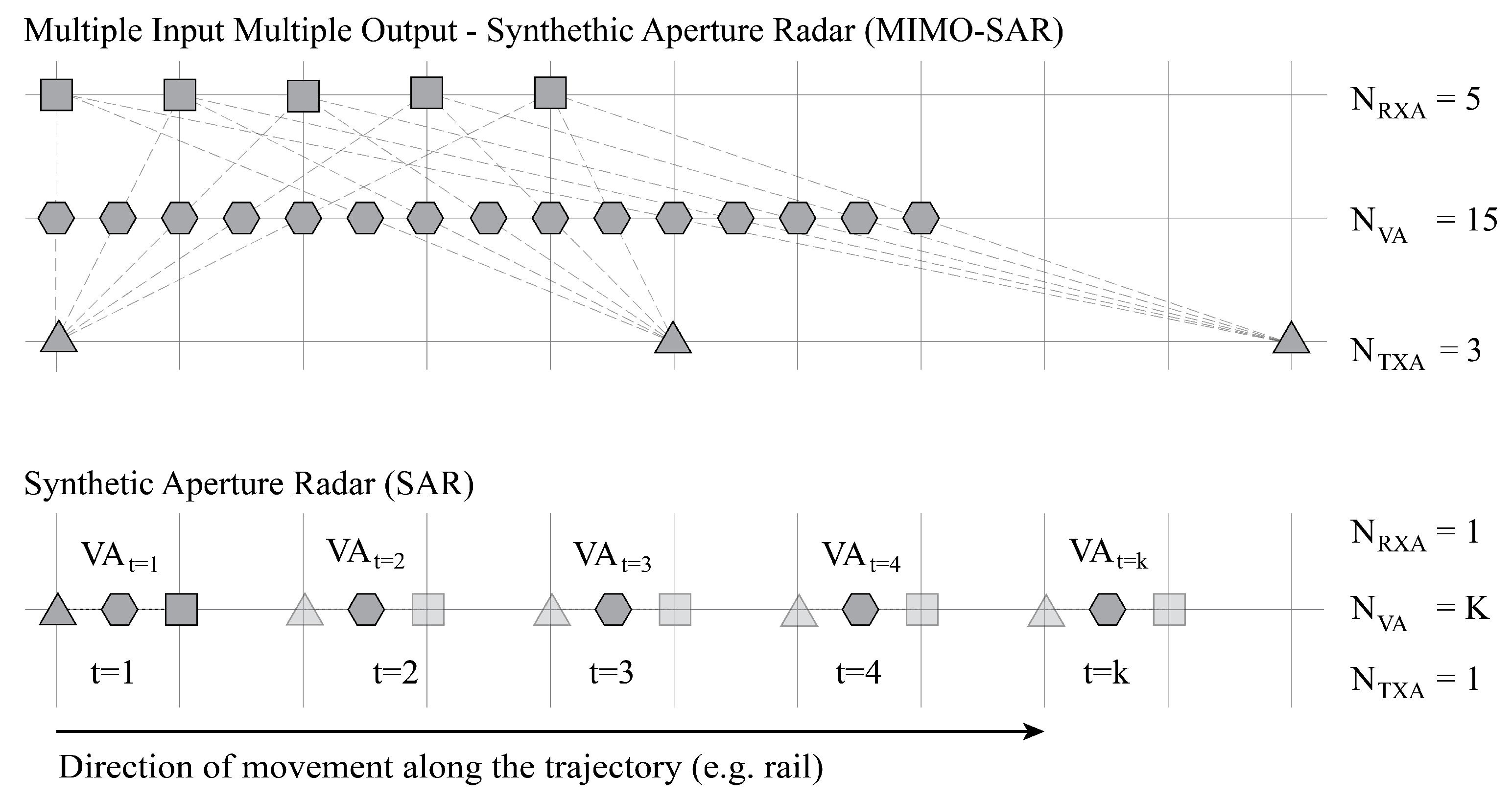
2.1. Antenna Configuration

MIMO-SAR employs frequency-modulated continuous waves (FMCW) that are emitted and received by multiple antennas installed in a fixed geometrical configuration. It has no moving parts and data acquisition can be performed faster compared to classical SAR systems. Each pair of the $N_{TXA}$ transmitting (TXA) and the $N_{RXA}$ receiving antennas (RXA) results in one virtual antenna (VA). If the physical antennas are spatially distributed in such a way, that every resulting VA is at a unique position, the MIMO-SAR system can acquire

$$N=N_{TXA}·N_{RXA}$$

(1)

independent measurements [32,34]. This concept is illustrated in Figure 1, where five equal-spaced RXA and three TXA create a pattern of 15 unique and linearly spaced VA. The observations can be distinguished through separation of the signals employing a time-division or frequency-division multiple-access approach. In the first case, all TXA emit at the same frequency but at different times and in the second case all TXA emit at the same time but with different frequencies.

To achieve the same acquisition geometry with a classical SAR system, the TXA-RXA pair of the SAR system needs to be moved over the full length of the path traced by the VA. This is time consuming and requires a positioning system achieving an accuracy on the order of a fraction of the wavelength.

The geometrical configuration of the MIMO-SAR system illustrated in Figure 1 exhibits co-linearly arranged antennas; consequently also the VA are linearly arranged. A horizontal linear arrangement of VA allows distinguishing horizontal angles ${\theta }_i$ of arrival (i.e., parallel to antenna orientation) but not the elevation of the arriving signal (i.e., orthogonal to antenna orientation). This deficiency can be alleviated by having the VA cover a two-dimensional area instead of being distributed along a line. Each unique VA has a different distance to the measured object and combining these observations allows to estimate the angle of arrival (Section 2.2). The capability to distinguish multiple targets w.r.t. their angle and range depends on the number of VA and the bandwidth of the emitted chirp (Section 2.3).

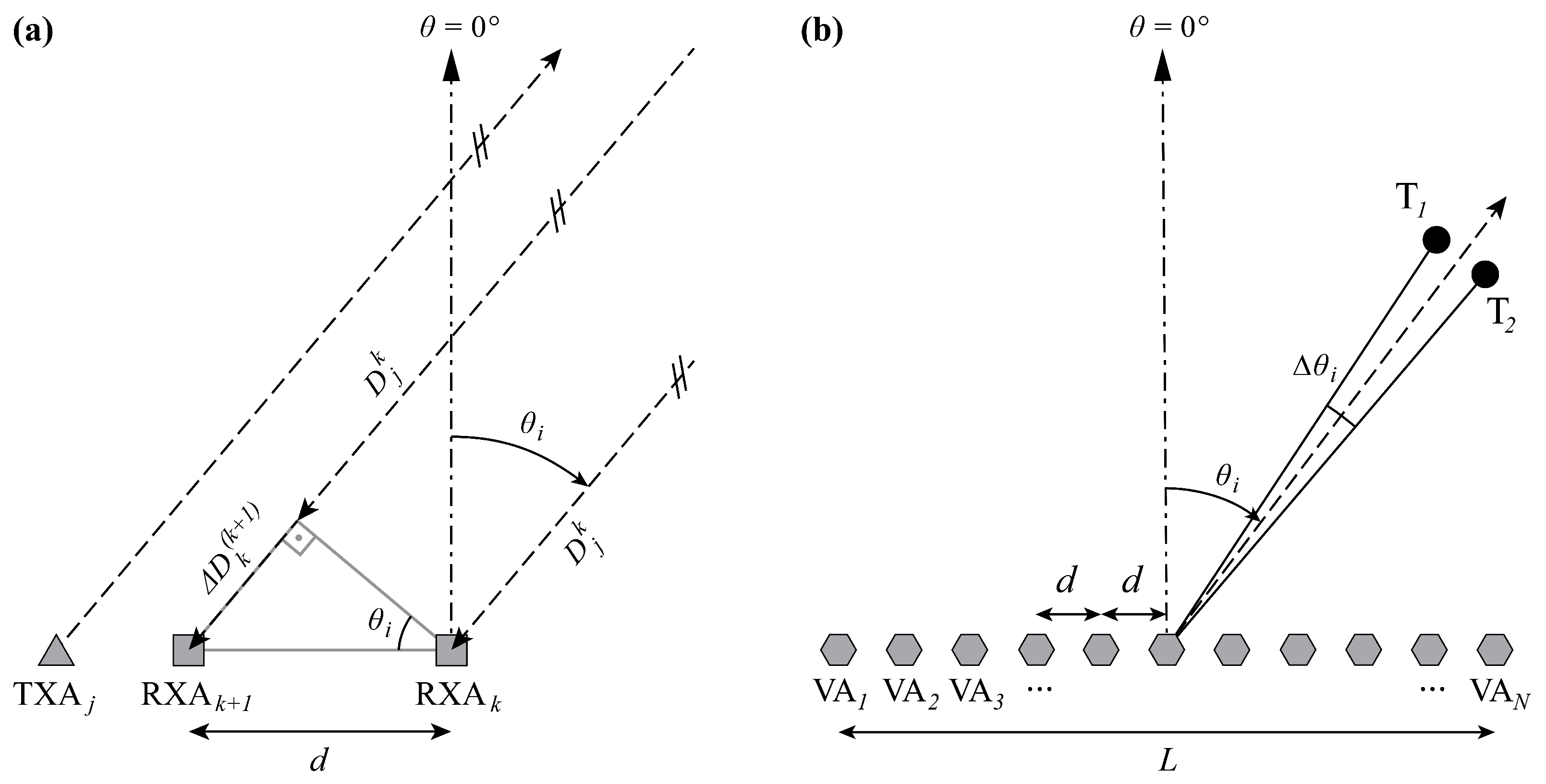
2.2. Angle Estimation and Field of View

For MIMO-SAR systems, every receiving antenna registers the backscattered signals of all the transmitting antennas. Suppose that two RXA separated by a distance d as illustrated in Figure 2a are receiving a signal scattered back from an object much further away than the length L of the synthetic aperture. Then the angle $\theta$ of the received backscattered signals is approximately equal for both RXA and the difference in travelled distance is $\Delta D=d·sin\left(\theta \right)$. This difference in distances corresponds to a phase difference $\mathsf{\Phi }$ of

$$\mathsf{\Phi }=\frac{2\pi }{\lambda }·d·sin\left(\theta \right)$$

(2)

between the two adjacent antennas, where $\lambda$ denotes the wavelength of the carrier wave. By solving Equation (2) for the angle of arrival $\theta$, one finds

$$\theta =si{n}^{-1}\left(\frac{\mathsf{\Phi }·\lambda }{2\pi ·d}\right).$$

(3)

Any phase difference $\mathsf{\Phi }$ derived as the argument of a complex number is bound to lie in the interval $(-\pi ,\pi ]$. Replacing $\mathsf{\Phi }$ in Equation (3) with $\pm \pi$ gives the angular field of view ${\theta }_{FOV}$ of

$${\theta }_{FOV}=\pm si{n}^{-1}\left(\frac{\lambda }{2·d}\right),$$

(4)

whose maximum span of $\pm {90}^{\circ }$ is achieved if the antennas are separated by $d=\lambda /2$ [35], p. 2f.

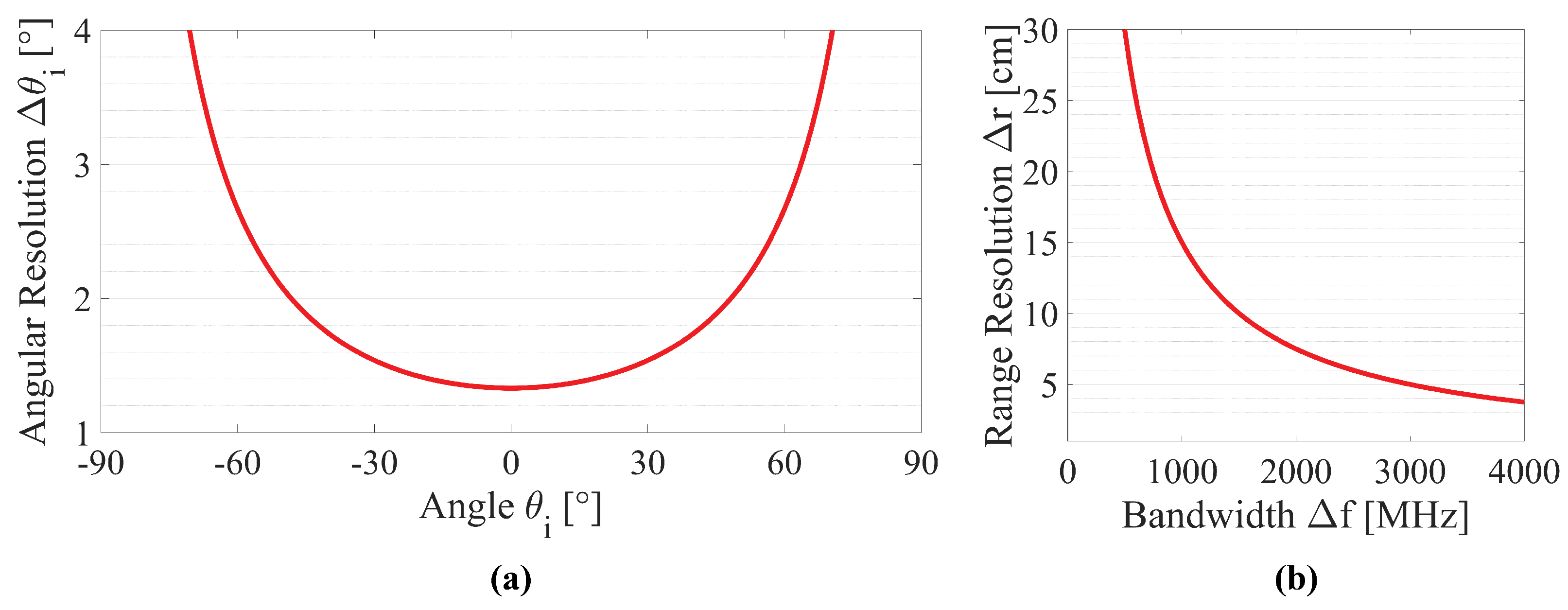
2.3. Angular and Range Resolution

The angular resolution of a SAR configuration depends on the length L of the synthetic aperture. Two objects at the same distance (Figure 2b, T₁ and T₂) will have distinct peaks in an angular matrix of length M, if their angular separation $\Delta {\theta }_i$ is

$$\Delta {\theta }_i\ge \frac{\lambda }{M·d·cos\left({\theta }_i\right)},$$

(5)

where $\lambda$ is the wavelength of the carrier frequency and ${\theta }_i$ the angle in azimuth direction with $\theta =0^{\circ }$ at boresight [35], p. 11. Achieving the maximum possible field of view (Equation (4)) and avoiding grating lobes [36], p. 307 requires that the distance between each acquisition should be evenly distributed and spaced by $\lambda /2$. This simplifies the equation and leads to

$$\Delta {\theta }_i\ge \frac{2}{M·cos\left({\theta }_i\right)}$$

(6)

and shows that the angular resolution is inversely proportional to the number of acquisitions along the synthetic aperture and degrades with larger azimuth. Assuming a sensor (i.e., TIDEP-01012) with 86 VA separated by $\lambda /2$ and based on Equation (6), the angular resolution in azimuth direction is $1.{33}^{\circ }$ in the direction corresponding to ${\theta }_i=0^{\circ }$ and degrades towards ${\theta }_i={90}^{\circ }$ as can be seen in Figure 3a.

The range resolution $\Delta r$ for a FMCW radar instrument is inversely proportional to the bandwidth $\Delta f$ of the chirp and can be computed as

$$\Delta r=\frac{c}{2·\Delta f},$$

(7)

where c denotes the speed of light [37]. The influence of the bandwidth on the range resolution can be seen in Figure 3b.

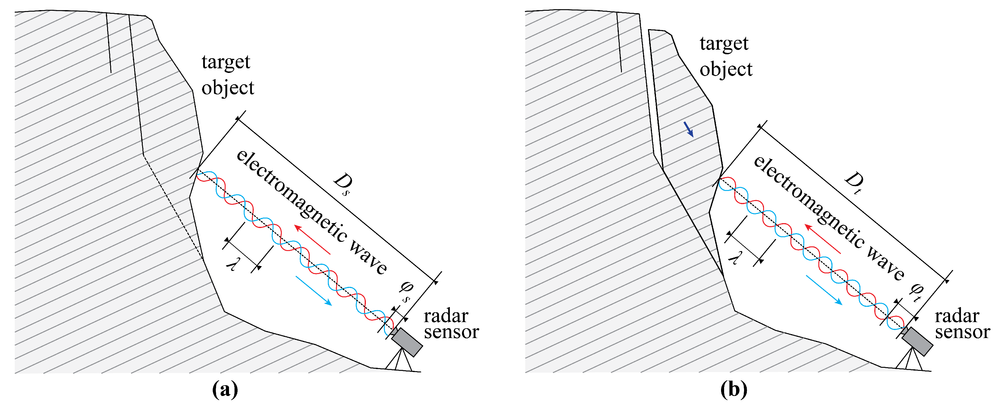
2.4. Radar Interferometry

The usual output of a radar acquisition is a single look complex ($SLC$) matrix. It represents the observations by associating complex numbers to the signals backscattered from objects located in a certain region in the physical world (Figure 4a). Those signals are assigned to bins which constitute the basic geometric building blocks of an SLC and each represent an area in the physical world with the smallest extent still resolvable. Consequently, an SLC is a complex-valued matrix of size $M\times N$, where M is the number of bins in azimuth direction and N is the number of bins in range direction (Figure 4b,c). Signals whose origins cannot be distinguished due to the finite spatial resolution as discussed in Section 2.3 are accumulated and the resulting single complex number encoding the superposition of signals is assigned to the corresponding bin. Every object within a bin $(k,l)$ at time t is contributing to the signal expressed as the complex value

$$SL{C}_t(k,l)=a+bj=Aexpj\varphi ,$$

(8)

where a and b denote the real and imaginary parts of the complex number and j is the imaginary unit. The amplitude $A=\sqrt{a^2+b^2}$ indicates the strength of the reflected signal depending on the orientation and material properties of the objects within the bin. In contrast, the complex number’s phase $\varphi =arctan2(b,a)$ encodes information about the distances between objects and radar. The exact relationship is

$$\varphi =\frac{(2·\pi )·(2·D)}{\lambda }(mod2\pi ),$$

(9)

with $\lambda$ as the wavelength of the emitted electromagnetic wave and $2·D$ the distance from the sensor to the target and back again. Consequently, TRI can detect an object’s movements by relating changes of distances $D_s$ and $D_t$ between sensor and object at epochs s and t to changes in the observed phase, see Figure 5. The equation

$$\begin{array}{cc}\hfill D_t-D_s=\Delta D_{st}& =\frac{\lambda }{4\pi }\Delta {\varphi }_{st}+\frac{n}{2}\lambda ,n\in \mathbb{Z}\hfill \end{array}$$

(10)

$$\begin{array}{cc}\hfill \Delta {\varphi }_{st}& =arctan2\left(Im({\overline{SLC}}_s\circ SL{C}_t),Re({\overline{SLC}}_s\circ SL{C}_t)\right)\hfill \end{array}$$

(11)

relates the real and imaginary parts of the complex interferogram ${\overline{SLC}}_s\circ SL{C}_t$, formed via pointwise multiplication of appropriately conjugated SLC_s, to the interferometric phase $\Delta {\varphi }_{st}$. The latter in turn depends on the changes of geometry that impart changes $\Delta D_{st}$.

This equation also shows a limitation of the interferometric displacement measurements. The displacement measured by evaluating the interferometric phase extracted from two SLC’s only coincides with the actual displacement if the latter one’s absolute value is smaller than $\lambda /4$. If it is larger, then phase unwrapping has to be performed, see e.g., [38]. Observations carried out over longer periods of time lead to time series of displacement observations that can be accumulated to total displacements exceeding $\lambda /4$.

3. Experiments

Firstly, we acquire and analyse measurements in a static indoor environment, in order to assess the stability and noise level of the phase observations (hereafter Indoor Static). Subsequently, in a second indoor experiment the instrument’s capabilities to detect actual deformations are assessed under relatively stable environmental conditions (herafter Indoor Dynamic). Finally, we investigate the same capabilities in an outdoor environment featuring various weather conditions mimicking a potential real-case scenario for SHM (herafter Outdoor Dynamic).

3.1. Experimental Device

We carry out our experimental investigation using a Texas Instruments TIDEP-01012 MIMO-SAR system. It consists of a radiofrequency board (MMWCAS-RF-EVM) and a digital signal processing board (MMWCAS-DSP-EVM), see Figure 6. The key modules of the radiofrequency board are 4 AWR1243 chips with each having 3 transmitting and 4 receiving channels operating in the frequency range between 76 and 81 GHz. The TIDEP-01012 has 12 transmitting (TX) and 16 receiving (RX) antennas and their arrangement results in a virtual antenna pattern consisting of 86 unique, linearly distributed, and equally $(\lambda /2)$-spaced antennas. According to Equation (6), this configuration provides a maximum azimuth angular resolution of $1.{33}^{\circ }$ at azimuth $0^{\circ }$.

The system allows acquisitions with a temporal resolution as high as milliseconds although the amount of generated data can be prohibitive. Due to onboard disk limitations, the continuous observation period is bounded to approximately 21 min when the temporal sampling density is set to 400 Hz. This is the default value used consistently across our experiments unless otherwise noted.

The instrument supports a wide range of chirp configurations with adjustable start frequency, frequency slope, sampling rates, and various secondary parameters. Based on the chirp settings, it can be used in long- (<350 m) or short-to-medium-range (<150 m) modes. For subsequent investigations, we deploy the instrument in short-to-medium-range mode.

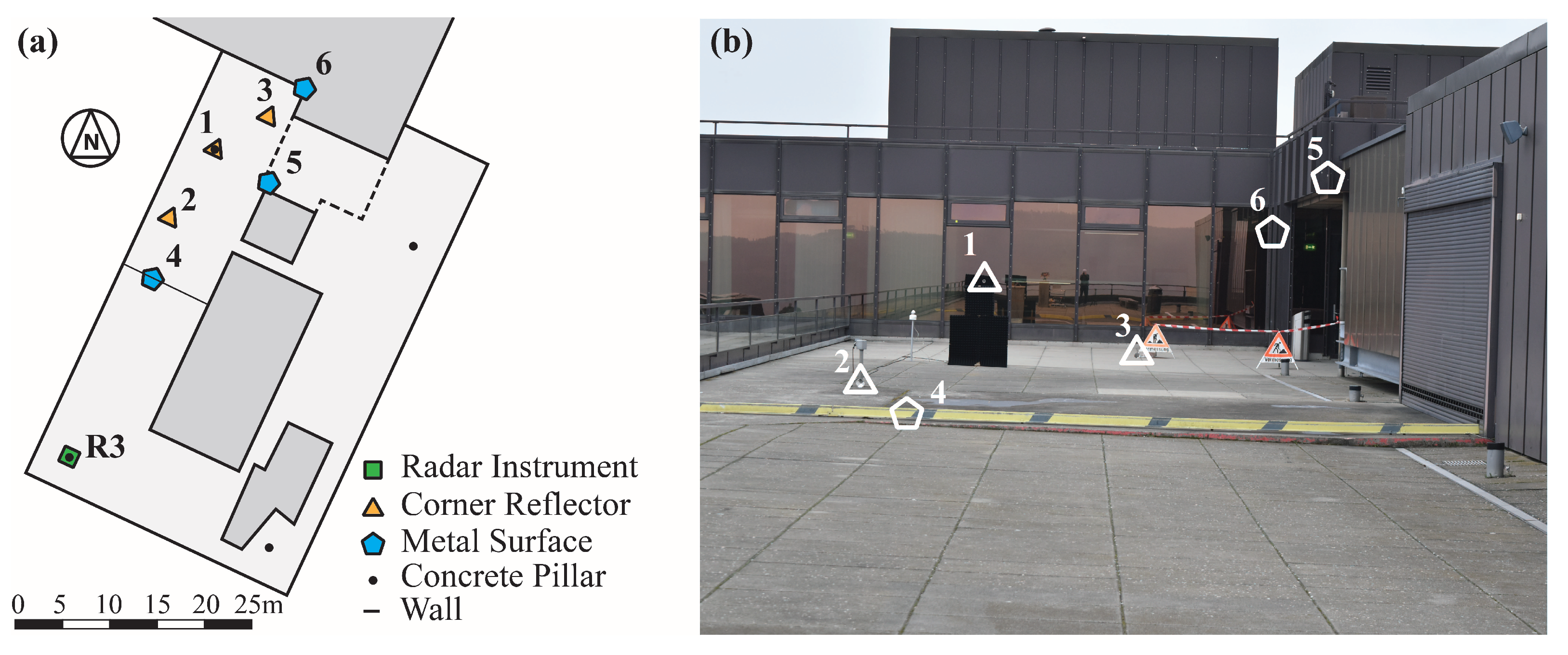
3.2. General Experimental Setup

To reliably quantify the capabilities of the radar instrument for measuring displacements, we require that the relative positions in our experimental setup are known with an accuracy at least one order of magnitude higher than the radar’s expected accuracy. Based on previous research [25,32,33], the accuracy of deformation measurements is not expected to be better than 10 μm. For this reason, we used the motorized translation stage ThorLabs MTS50/M-Z8. It has a bidirectional repeatability of 0.8 μm and an absolute positioning accuracy of 290 μm [39]. We mounted a small square corner cube with an edge length of 40 mm onto this translation stage and subsequently moved it in a stepwise fashion.

To reduce inter-channel mismatch, we follow the calibration procedure outlined in the Texas Instruments’ mmWave Studio software [40]. Further configuration options are accessible via lua scripting. We chose a chirp bandwidth of 1280 MHz leading to a range resolution of 11.7 cm and a maximum distance of 60 m. These choices present a trade-off between distance coverage and high range resolution. They allow a single acquisition to span the whole extent of the delivery hall chosen for the experiments while still guaranteeing identifiability of the Pixels containing primarily the corner cube reflector. A detailed summary of the relevant parameters can be seen in

Table 2. Parameters for the experiments.

Parameter	Indoor Static	Indoor Dynamic	Outdoor Dynamic
Center Frequency $f_c$ [GHz]	77.72	77.72	77.72
Frequency Slope $s_c$ [MHz/μs]	40	40	40
Idle Time [μs]	2	2	2
ADC Start Time [μs]	2	2	2
ADC Samples $N_{ADC}$ [-]	512	512	512
Sample Frequency [kHz]	16,000	16,000	16,000
Ramp End Time [μs]	35	99	99
Acquisition Rate [Hz]	400	20	10

. The parameters for Indoor Static were chosen to allow for as many acquisitions as possible in a short period of time. We decided to restrict the repetition rate to a maximum of 400 Hz due to limited on-board storage and total observation time even though higher temporal resolutions are possible. The parameters of Indoor Dynamic and Outdoor Dynamic have been chosen to be able to acquire multiple repetitions of translation stage movement at once and have therefore only acquisition rates of 10 and 20 Hz. For all the experiments, the TIDEP-01012 was installed on a tripod and controlled with a laptop with power supplied directly by the power grid. Whenever beneficent, we placed small (40mm) and large (80mm) squared corner cubes into the observed scene.

3.3. Indoor Experiments

To estimate an upper bound for the accuracy of the radar in situations with negligible meteorological variations, we gather data in a stable indoor setting in an underground delivery hall. This environment features relatively stable atmospheric conditions and is sufficiently large to enable measurements over a range of 60 m. Two experiments were carried out in this setting.

The first experiment (Figure 7b) features the radar instrument (R1) transmitting down a long hallway. Two small (S1/S2) and two large (L1/L2) corner cubes were placed on the ground in distances between 17 and 46 m and separated by about 10 m from each other. The radar instrument acquired SLC_s with a rate of 400 Hz and had to restart the acquisition process after each cycle due to the previously mentioned on-board disk constraints. The restarting procedure takes about four seconds and causes small data gaps in the time series.

For the second experiment, the instrument was set up at a different location (Figure 7c, R2) and aligned towards a small corner cube mounted on the translation stage (Figure 7c), (1) located in a distance of about 19 m. Another small corner cube at location (3) and a large corner cube at the pillar (2) were also included for comparison. The translation stage was programmed to move the corner cube in steps of 25 μm from 0 to 10 mm and back to 0 mm. It maintained each position for two seconds before moving to the next one allowing the radar to collect 40 observations at each position.

3.4. Outdoor Experiments

The third experiment was carried out on a terrace and aimed to assess the performance of the instrument in an outdoor environment featuring uncontrolled and varying meteorological conditions. The specific conditions for the different acquisitions corresponding to this experiment are detailed in

Table 3. Weather conditions at the dynamic experiments carried out between October 2020 and January 2021.

Day	Location	Weather	Temperature [°C]	Humidity [%]	Pressure [hPa]
17 October 2020	Indoor	-	16.0–16.8	49.9–50.7	$957.8$
14 November 2020	Outdoor	Sunshine	15.8–16.6	40.7–44.8	$956.5$
14 December 2020	Outdoor	Fog	3.4–4.6	80.3–84.9	$951.5$
18 December 2020	Outdoor	Fog	3.8–4.8	82.3–90.9	$960.0$
5 January 2021	Outdoor	Cloud	0.3–0.6	67.8–69.8	$946.4$

. Figure 8 shows the experimental setup. The radar instrument was mounted on a concrete pillar at location (R3) and aligned towards a second pillar at (1), which hosted a translation stage with a corner cube on top. The pillar was covered with absorbing mats to reduce its backscatter and to isolate the corner cube. Two large corner cubes on the ground (2/3) and three natural reflectors (4/5/6) were also introduced. Bins associated with those targets were chosen for assessing the long-term stability of the measurements. A Reinhardt DFT1M meteo instrument [41] was placed on site and once every minute measured temperature, air pressure, and relative humidity (Table 3). SLC_s were acquired with a rate of 10 Hz. The translation stage moved in steps of 500 μm from 0 to 50 mm and back to 0 mm. At each position, the translation stage waited between two and three seconds leading to 20–30 observations per position.

4. Results and Discussion

The results obtained from the experiments described above are shown and discussed in this section. Section 4.1 describes the impact of meteorological effects on the observations and Section 4.2 quantifies instrument-induced effects. Quantifying the phase stability requires a separation of uncertainties induced by the environment and by the instrument. This is done by investigating the impact of the measurement configuration on the phase stability in Section 4.3, followed by an assessment of the range of detectable displacements and their accuracy (Section 4.4).

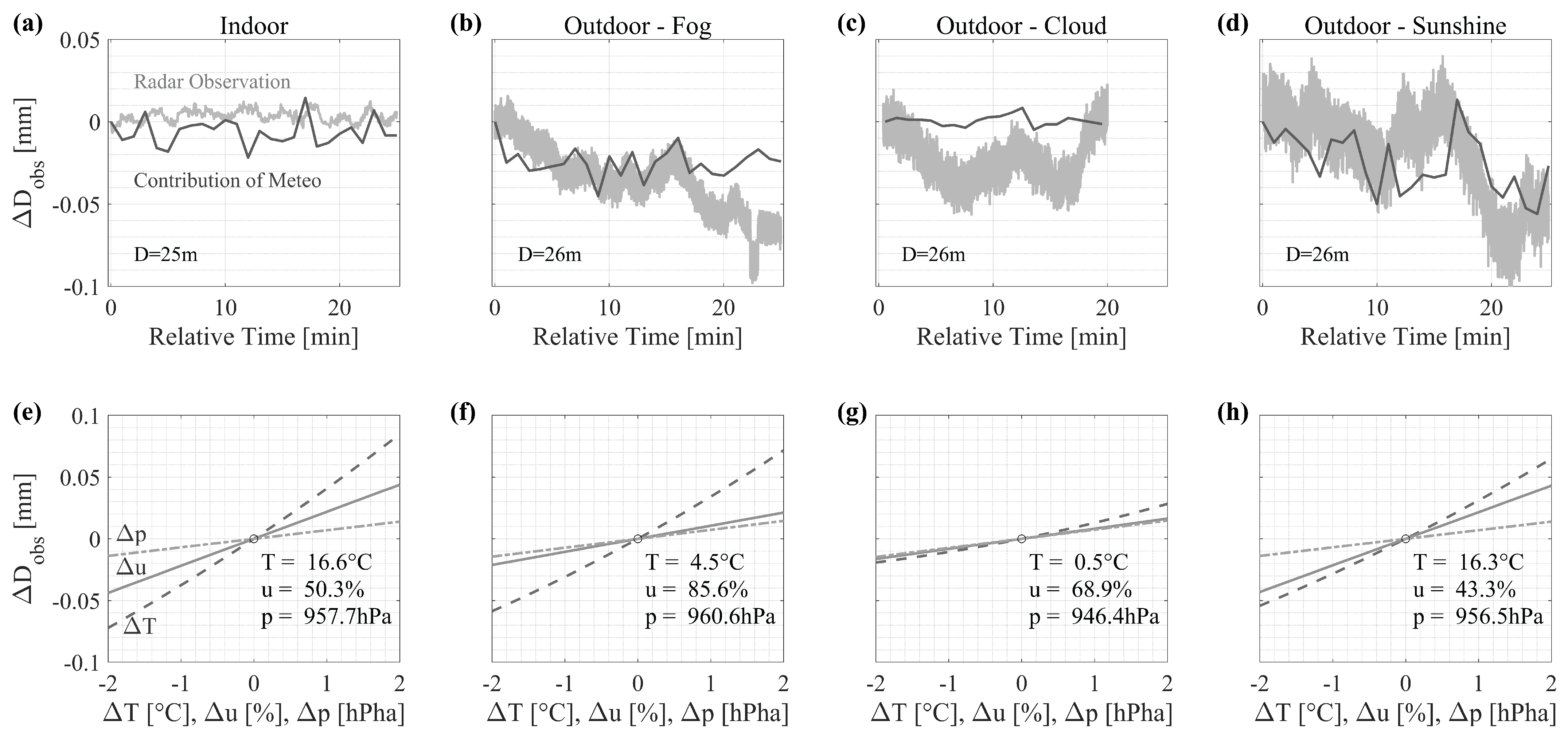
4.1. Meteorological Impacts

The results of indoor and outdoor measurements alike are two-dimensional complex matrices containing information about the amplitude and phases of the waves scattered back from the objects captured by the radar. An amplitude and phase image can be seen in Figure 9, showcasing the distribution of amplitudes as measured in the outdoor experiment and the phase differences occurring during subsequent acquisitions.

If the location of an object relative to the radar instrument does not change and all other influences are constant, the phase value in the corresponding bins of the radar image remains the same for subsequent measurements. However, in most practical situations, drifts caused by changing environmental conditions (e.g., temperature and humidity [42,43]) as well as instrumental effects (e.g., stability of tripod and sensor chip temperature) are to be expected on top of noise. Figure 10a–d shows examples of time series of phase values acquired in the previously described indoor and outdoor experiments. Each of these time series corresponds to a bin representing a reflector (Figure 7, No. 6 and Figure 8, No. 2) which did not move with respect to the radar instrument during the chosen time windows of about 25 min. For the indoor case, Figure 10a, the radar results confirm this stability: the accumulated displacements $\Delta D_{\mathrm{obs}}$ remain within a band of only about 10 μm. We find much larger variations both in terms of noise level and drift of $\Delta D_{\mathrm{obs}}$ for the three outdoor cases (Figure 10b–d) with apparent, accumulated displacements reaching 100 μm.

We estimated the refraction index based on the measured meteorological conditions and calculated the contribution of the atmospheric changes to the phase observations using Equation (9) [44]. These calculated meteorological contributions have not been used to correct the radar data but are instead plotted separately in Figure 10a–d. Some correlation between the two curves can be seen. However, the calculated meteorological effects do not fully explain the drifts of the interferometric phase values. This is likely due to the high sensitivity of the phase values with respect to the atmospheric conditions and the uncertainty of the meteorological data.

Figure 10e–f shows the impact of deviations in temperature, relative humidity, and barometric pressure on the phase measurement for each of the four experiments. The phase measurements are sensitive with respect to changes in all three parameters. However, the impact of temperature and humidity changes is particularly pronounced, and different for the different experiments. A change of only 2% in relative humidity causes an apparent displacement of about 20 μm at low temperatures (0 to 5 °C) as in the two outdoor cases Figure 10b,c, and about 45 μm at the higher temperature during the two other experiments (Figure 10a–d).

The high-quality Reinhardt DFT1M instrument used for collecting the meteorological data has a specified measurement accuracy of 0.3 °C for temperature, 2.0% for relative humidity, and 0.8 hPa for air pressure [41]. This results in an uncertainty of several tens of microns of the meteorological effects calculated from the meteorological data, and thus is a potential explanation for the magnitude of the deviations visible in Figure 10a–d. However, at least for the outdoor experiments, these deviations have clear systematic patterns, and this hints at a more fundamental challenge.

The meteorological measurements describe the atmospheric conditions at the location of the meteo sensors, but the atmospheric impact on the radar measurements is the accumulated impact along the radar signal paths from the instrument to the reflecting surfaces and back. If the meteorological measurements are not representative for the average conditions along these signal paths, the calculated meteorological effects will be biased. The fairly good agreement between the variability of the calculated meteorological effects and the measurements in the indoor experiment suggests that the meteo measurements were representative for the signal paths in this case, while the systematic deviations in the outdoor cases can be attributed to the fact that the meteo measurements in one location were not representative for the conditions along the signal path. This is particularly corroborated by the case in Figure 10b where passing swaths of fog between the instrument and the reflector were visually observed and the corresponding variations of humidity (for which no measurements exist) qualitatively explain the variability of the radar measurements.

We conclude that changes in meteorological conditions significantly affect the displacements observed by a radar interferometer and may cause biases by far exceeding the otherwise attainable noise levels. Since it is usually not possible to measure the meteorological conditions along the signal paths with sufficient accuracy, atmospheric effects will be a dominant source of deviations in many applications of radar-interferometry. However, while MIMO-SAR measurements are not different from other radar measurements in that respect, the atmospheric impact is typically less detrimental for short distances and for short time intervals such that MIMO-SAR-based vibration and deformation measurements are possible with sub-mm accuracy for distances of up to about 200 m despite uncompensated atmospheric effects, as the above examples suggest.

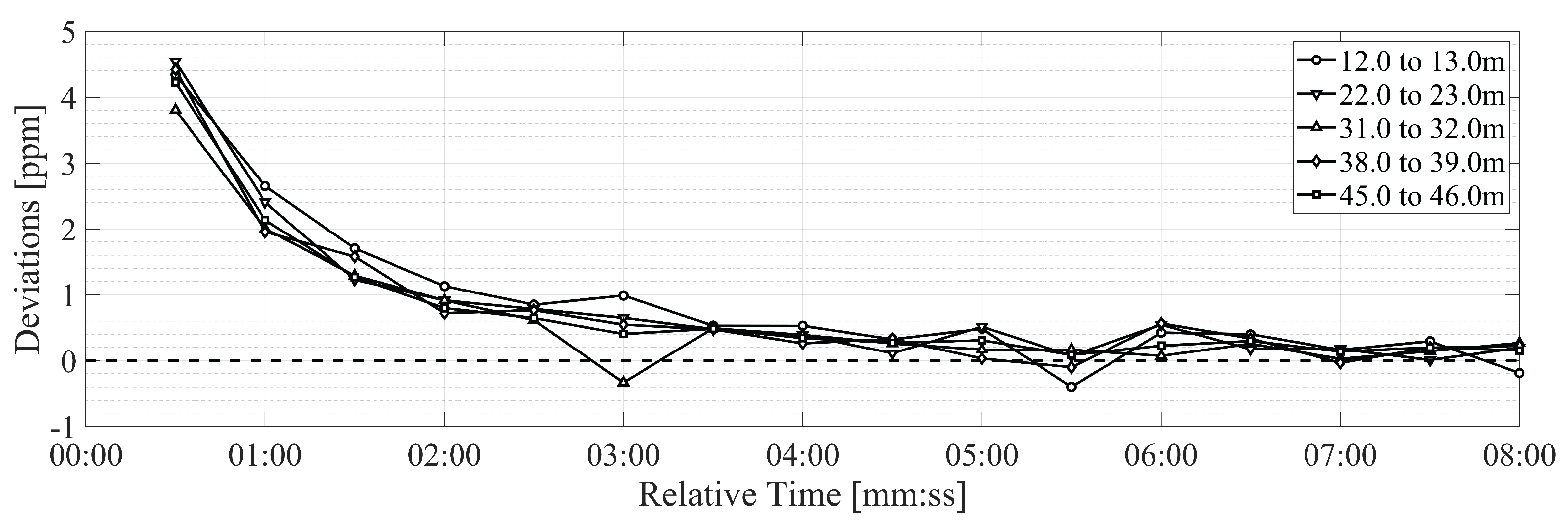
4.2. Quantification of Systematic, Instrument-Induced Effects

The meteorological conditions in the indoor environment are stable over short periods of time, as seen in Figure 10a. The influence of atmospheric effects is therefore negligible and instrumental effects are dominant. We process the dataset acquired in the static indoor experiment (Indoor Static) to analyse instrument-induced uncertainties. We selected bins representing stable reflectors with good signal-to-noise ratio as encoded in the amplitude dispersion index $ADI={\sigma }_A/{\mu }_A\le 0.1$ [45] relating the standard deviation ${\sigma }_A$ and the mean ${\mu }_A$ of measured amplitudes. The strong and stable reflectors extracted with this approach are mostly metallic objects like containers, meshed fences, and corner cubes as well as corners of concrete and brick walls.

We unwrapped the observed phases and converted them to a metric scale to uncover time-dependent patterns in the cumulative displacements calculated from the interferometric phases. The disjoint acquisition sets were connected with each other by extrapolating a second order polynomial trend over the data gaps caused by the restarts mentioned in Section 3.3. As a further step, we investigated the averaged measured distance change over 30 s and noted an approximate linear dependency on distance. We present the quotient in Figure 11.

The resulting measurements from stable reflectors exhibit a systematic drift at the beginning of the acquisition period; that drift disappears with increasing observation time. We observed that these apparent changes in distance are linearly dependent on distance, which points towards a varying scale error. A plausible cause for the observed drifts is a frequency shift during warming-up of the crystal oscillator embedded in the radio frequency board. During the experiments, the board heated up from a temperature of the environment (16 °C) to a temperature of 50 °C in a matter of minutes after initialization. The observed scale changes of about 4 ppm are explainable by a shift in frequency of 0.35 MHz—a plausible deviation expected of the crystal oscillator embedded in the TIDEP-01012 MIMO-SAR system [46]. We have identified three practical approaches to mitigate this shift in frequency and we applied the last mitigation procedure for the following investigations.

•

Mounting the radar in a protective box with active heating to stabilize the operating temperature.

•

Estimating the relative frequency drift based on known stable points and removing it from all observations.

•

Ignoring the first three minutes of acquisitions.

4.3. Quantification of Phase Stability

To analyse the temporal variability of the random instrumental effects, we compute the Allan deviation (ADEV) of the time series of cumulative displacements. The Allan deviation is defined as

$$ADEV={\sigma }_{\mathrm{ADEV}}\left(\tau \right)=\sqrt{\frac{1}{2}\langle {({\overline{y}}_{n+1}-{\overline{y}}_n)}^2\rangle }$$

(12)

with ${\overline{y}}_n$ denoting in this case the average displacement over the n-th observation period of duration $\tau$ and $\langle .\rangle$ denoting the expectation operator.

The Allan Deviation computed on the displacement data is invariant to constant biases and linear drifts, helping in understanding the spectral distribution of noise and higher order drifts [47]. This in turn enables quantifying the expected precision as a function of integration time, which can be selected by averaging subsequent displacement observations.

We calculated the Allan Deviation using the data gathered during the static indoor experiments, thereby minimizing the impact of atmospheric influences on the measurements and isolating internal effects; namely measurement noise and short-term drifts due to clock instabilities. Figure 12 shows the computed ADEV as a function of the observation period for a sampling rate 400 Hz over a time-series of 8 $\min$. The results show a standard deviation of 18.5 μm for the individual measurements acquired every 2.5 ms. The slope of the ADEV with increasing observation time until approximately 1 s indicates that white noise dominates for frequencies higher than 1 Hz. Subsequent measurements are therefore highly uncorrelated within this time frame, and increasing integration time up to 1 s improves precision effectively. Considering the application focus of this work on high-frequency monitoring, only integration times up to some tens of ms are relevant. If allowed by the dynamic requirements of other applications, however, noise absorption can be maximized by integrating approximately 1 s, yielding minimum standard deviations of about 1.5 μm. Averaging individual measurements over more than 1 s is inefficient due to higher-density low-frequency noise components and drifts dominating the deviations. The maximum deviation introduced by these slower processes shall be assessed via stability tests over longer periods (see Figure 10a–d). The results of this test under stable meteorological conditions show peak-to-peak variations of 100 μm over 25 min. Stability analysis over longer periods is so far hindered by the prohibitively large amount of generated data, and is planned for future work once this practical limitation is resolved.

4.4. Detection Limits and Relative Accuracy

We consider MIMO-SAR phase masurements as superpositions of displacements and unwanted effects. As a high signal-to-noise ratio benefits extracting displacements from phase measurements, the characteristics of the noise distribution impact the size of minimum detectable displacements (MDD). To provide confidence intervals depending on the phase noise floor, we model displacement measurements $\Delta D^k,k=1,\dots ,N$ as distributed with constant mean and variance ${\sigma }_{\Delta D}^2$. They are assumed to be derived from k pairs of interferometric phase observations ${\varphi }_1^k,{\varphi }_2^k$ that are related to $\Delta D^k$ via the wavelength $\lambda$ as $\Delta D^k=\lambda {\left(4\pi \right)}^{-1}({\varphi }_1^k-{\varphi }_2^k)$ with the standard deviations ${\sigma }_{\Delta D}$ and ${\sigma }_{\varphi }$ also being linked by this linear equation. Assuming uncorrelated white noise, the average displacement $\overline{\Delta D}=N^{-1}{\sum }_{k=1}^N\Delta D^k$ as computed from N samples has the standard deviation

$$\begin{array}{c}\hfill {\sigma }_{\overline{\Delta D}}={\left[\frac{{\lambda }^2}{N^2{\left(4\pi \right)}^2}\sum _{k=1}^N({\sigma }_{\varphi }^2+{\sigma }_{\varphi }^2)\right]}^{1/2}=\frac{\sqrt{2}\lambda }{4\pi \sqrt{N}}{\sigma }_{\varphi }.\end{array}$$

(13)

Defining the Nullhypothesis as the assertion that no displacement occurred, these relationships can be used to determine a well-behaved rejection criterion. Rejecting the Nullhypothesis and thereby diagnosing deformations if the measured phase differences imply a deformation in excess of $3{\sigma }_{\Delta D}$ ensures a rate of false positives of less than 0.3%. This criterion indicates the presence of deformation with relative certainty. Furthermore, any true underlying displacement whose absolute value is bigger than $6{\sigma }_{\Delta D}$ leads to measurements whose rejection probability is bigger than 99.7% and a rate of false negatives lower than 0.3 %. Therefore, any $|\Delta D|\ge$ MMD with

$$\begin{array}{c}\hfill \mathrm{MMD}=\frac{6·\sqrt{2}\lambda }{4\pi }{\sigma }_{\varphi }\end{array}$$

(14)

is detectable with less than the error rates mentioned above. The MMD decreases with a factor of $1/\sqrt{N}$ if the displacement estimate is a result of averaging N pairs of phase measurements exhibiting constant mean; this is the expected behaviour for observation times below 1 $\mathrm{s}$ as shown in Figure 12.

The variance of the phase measurements originates from random noise sources internal to the instrument and the variability of atmospheric conditions. We expect the instrumental noise sources to impact phase measurements by imparting a spatially and temporally uncorrelated zero-mean deviation to them. The variance of these deviations is typically larger for measurements with low amplitudes [45] for which we expect them to be the dominant source of uncertainty. Changes of meteorological conditions between consecutive measurements exhibit different behavior. Due to the variation of the refractive index depending on physical quantities and playing the role of a scale factor, atmospheric effects are temporally autocorrelated and increase in variance with increasing distance.

For the duration of short-term monitoring applications in a controlled environment, it is therefore reasonable to assume instrument noise to be the dominant factor hampering the detection of displacements. For longer term monitoring scenarios, detectable displacements are limited by the long-term stability of the measurements, mostly determined by the stability of the time-base of the system and meteorologically induced drifts whose severity increases with distance. Consequently, the Indoor and Outdoor datasets allow to empirically estimate the impact of both of these sources of error.

In the indoor environment featuring stable atmospheric conditions, we observe an empirical standard deviation of approximately 4 μm for a cluster of bins representing one corner cube. Based on the previous considerations this implies that a displacement of 35 μm can be detected with the probability of false positives and false negatives bounded from above by 0.3% when measuring with a sampling rate of 400 Hz. Averaging the phase measurements prior and posterior to the deformation for 1 s reduces the noise floor by an order of magnitude, thus decreasing the MMD to about 4 μm.

Measurements in the outdoor environment exhibited a standard deviation of approximately 8 μm for a cluster of bins representing one corner cube. This deviation, likely dominated by high-frequency atmospheric variability, implies a MMD of 70 μm or 7 μm after an integration time of 0.25 s. Figure 13 illustrates these choices to be rather conservative with displacements of 25 μm appearing to be easily resolvable for measurements in the indoor-environment.

These results indicate detectability of displacements in short-term monitoring applications. In order to assess the achievable relative accuracy taking into account long-term instabilities we repeated the outdoor experiment multiple times during various days and weather conditions (Table 3). We measured the relative positions of the corner reflector mounted on a translation stage upon which we compared the observed relative displacement with the calibrated translation stage positions. Figure 14 shows the position on the translation stage and the residuals of the radar observation with respect to the translation stage position.

A periodic deviation of the average residuals with a frequency of 3 cycles per 50 mm is clearly visible. This cyclic pattern also appeared during the calibration process of the translation stage overseen by a laser tracker with an accuracy of a few μm. This is most likely explained by manufacturing imperfections of the translation stage introducing deviations in the corner cube’s position. Aside from these contributions, the residuals are mostly lower than ±100 μm and have an RMSE of approximately 25 μm. They do not seem to be symmetrically distributed around 0 and show a degree of auto-correlation not consistent with them being independently and identically distributed white noise. These systematic deviations are likely attributable to persistent changes in the atmospheric conditions as shown in Section 4.1. These results show that detecting displacements in-between longer periods of time is strongly limited by the refractivity errors introduced by the variation of the meteorological conditions.

Lastly, we briefly mention that an upper boundary limiting detectability exists as well. If a displacement occuring between two acquisitions exceeds 1/4 of the center wavelength of the emitted chirp, the resulting phase differences cannot be converted to distances uniquely. For a W-band radar like the TIDEP-01012 operating at 79 GHz, this implies a maximum detectable displacement of 0.95 mm with larger displacements resolvable only when spatial information can be employed to perform phase unwrapping.

5. Conclusions

Multiple Input Multiple Output Synthetic Aperture Radar (MIMO-SAR) has emerged as a cost-efficient and easily deployable solution to implement terrestrial radar interferometry (TRI). It enables higher measurement rates than other terrestrial SAR approaches, which makes it potentially suitable for SHM tasks with demanding dynamics such as structure vibration measurements. Due to its novelty, however, the practical applicability of MIMO-SAR TRI to SHM still requires a better understanding of its accuracy limits and the effects impacting it. In this work, we contribute to this understanding by analysing and quantifying the sensitivity of displacement measurements. We carried out and analysed experiments with a commercial W-band MIMO-SAR system in indoor and outdoor environments with an acquisition frequency of up to 400 Hz.

We have shown that there are short- to long-term effects influencing the phase observations. On the short-term, instrumental uncertainties have been quantified by isolating atmospheric influences on a controlled indoor experiment. We analysed the noise spectral distribution of the displacement measurements via Allan Deviation. The results yield a standard deviation of ${\sigma }_{ADEV}=$ $18.5$ $\mathsf{\mu }$$\mathrm{m}$ for individual measurements acquired at 400 Hz. An optimal integration time of approximately 1 $\mathrm{s}$ was identified, reducing the standard deviation of estimated displacements to about ${\sigma }_{ADEV}=$ $1.5$ $\mathsf{\mu }$$\mathrm{m}$. The radar instrument is also likely influenced by a warm-up effect of the sensor itself, which causes temperature dependent frequency drift and influences the displacement measurements by 4.5 ppm in the first 30 s of measurements for an environmental temperature of 16 °C. That effect decreases continuously with acquisition time with the impact being lower than 0.5 ppm after a warm-up time of 3 min. The global uncertainty budget for larger time frames is dominated by changes of meteorological conditions with humidity and temperature being the dominant factors. A change of 2% in relative humidity in an environment of 16 °C causes a change of refractivity and leads to an apparent displacement of approx. 45 $\mathsf{\mu }$$\mathrm{m}$ at 25 $\mathrm{m}$.

For corner cubes, we were able to showcase detectability of displacements as small as 25 μm under stable weather conditions and 50 $\mathsf{\mu }$$\mathrm{m}$ during fluctuating weather conditions for distances smaller than 35 m. Based on the empirical standard deviations of the interferometric displacements, confidence intervals can be constructed. They indicate that with 99.72 % confidence, displacement measurements did not deviate from their expected value by more than 16 $\mathsf{\mu }$$\mathrm{m}$ in the indoor environment and 35 $\mathsf{\mu }$$\mathrm{m}$ in the outdoor environment exhibiting changing meteorological conditions. In the short-term, the displacement measurements are affected by phase noise and high-frequency meteorological changes. In the long-term, the accuracy is mostly dominated by changes in meteorological conditions. Generally, it decreases with distance. In our experiments, it was bound to ±100 $\mathsf{\mu }$$\mathrm{m}$ at a distance of approximately 25 $\mathrm{m}$.

These results indicate that highly accurate displacement measurements are possible by estimating and correcting or altogether avoiding meteorological and instrumental effects. Consequently, MIMO-SAR is a promising technology suitable for measuring short-term displacements as is necessary for the monitoring of bridge vibrations, dynamic load tests, or other applications featuring high temporal frequencies and sub-mm displacements. With these capabilities it is complementary to other established monitoring techniques, e.g., satellite-based InSAR which provides larger coverage and stability over longer time-spans but significantly coarser temporal and spatial resolution. It will thus be worth exploring in the future, how MIMO-SAR can be integrated with other sensors for comprehensive structural monitoring or even geomonitoring.

References

1. Massonnet, D.; Feigl, K.L. Radar interferometry and its application to changes in the Earth’s surface. Rev. Geophys. 1998, 36, 441–500. [Google Scholar] [CrossRef] [Green Version]
2. Monserrat, G.; Crosetto, M.; Luzi, G. A review of ground-based SAR interferometry for deformation measurement. ISPRS J. Photogramm. Remote Sens. 2014, 93, 40–48. [Google Scholar] [CrossRef] [Green Version]
3. Pepe, A.; Calò, F. A Review of Interferometric Synthetic Aperture RADAR (InSAR) Multi-Track Approaches for the Retrieval of Earth’s Surface Displacements. Appl. Sci. 2017, 7, 1264. [Google Scholar] [CrossRef] [Green Version]
4. Solari, L.; Del Soldato, M.; Bianchini, S.; Ciampalini, A.; Ezquerro, P.; Montalti, R.; Raspini, F.; Moretti, S. From ERS 1/2 to Sentinel-1: Subsidence Monitoring in Italy in the Last Two Decades. Front. Earth Sci. 2018, 6, 149. [Google Scholar] [CrossRef]
5. Caduff, R.; Schlunegger, F.; Kos, A.; Wiesmann, A. A review of terrestrial radar interferometry for measuring surface change in the geosciences. Earth Surf. Process. Landforms 2015, 40, 208–228. [Google Scholar] [CrossRef]
6. Pieraccini, M.; Miccinesi, L. Ground-Based Radar Interferometry: A Bibliographic Review. Remote Sens. 2019, 11, 1029. [Google Scholar] [CrossRef] [Green Version]
7. Sun, S.; Petropulu, A.P.; Poor, H.V. MIMO Radar for Advanced Driver-Assistance Systems and Autonomous Driving: Advantages and Challenges. IEEE Signal Process. Mag. 2020, 37, 98–117. [Google Scholar] [CrossRef]
8. Casas, J.R.; Cruz, P.J.S. Fiber Optic Sensors for Bridge Monitoring. J. Bridge Eng. 2003, 8, 362–373. [Google Scholar] [CrossRef] [Green Version]
9. Chen, Y.; Xue, X. Advances in the Structural Health Monitoring of Bridges Using Piezoelectric Transducers. Sensors 2018, 18, 4312. [Google Scholar] [CrossRef] [PubMed] [Green Version]
10. Yu, J.; Meng, X.; Shao, X.; Yan, B.; Yang, L. Identification of dynamic displacements and modal frequencies of a medium-span suspension bridge using multimode GNSS processing. Eng. Struct. 2014, 81, 432–443. [Google Scholar] [CrossRef]
11. Sabato, A.; Niezrecki, C.; Fortino, G. Wireless MEMS-Based Accelerometer Sensor Boards for Structural Vibration Monitoring: A Review. IEEE Sens. J. 2017, 17, 226–235. [Google Scholar] [CrossRef]
12. Ha, D.; Park, H.; Choi, S.; Kim, Y. A Wireless MEMS-Based Inclinometer Sensor Node for Structural Health Monitoring. Sensors 2013, 13, 16090–16104. [Google Scholar] [CrossRef] [Green Version]
13. Lienhart, W.; Ehrhart, M.; Grick, M. High frequent total station measurements for the monitoring of bridge vibrations. J. Appl. Geod. 2017, 11, 1–8. [Google Scholar] [CrossRef]
14. Gordon, S.; Lichti, D.; Stewart, M. Application of a high-resolution ground-based laser scanner for deformation measurements. In Proceedings of the 10th FIG International Symposium on Deformation Measurements, Orange, CA, USA, 19–22 March 2001. [Google Scholar]
15. Pieraccini, M.; Fratini, M.; Parrini, F.; Atzeni, C. Dynamic Monitoring of Bridges Using a High-Speed Coherent Radar. IEEE Trans. Geosci. Remote Sens. 2006, 44, 3284–3288. [Google Scholar] [CrossRef]
16. Jung, J.; Kim, D.-J.; Palanisamy Vadivel, S.K.; Yun, S.-H. Long-Term Deflection Monitoring for Bridges Using X and C-Band Time-Series SAR Interferometry. Remote Sens. 2019, 11, 1258. [Google Scholar] [CrossRef] [Green Version]
17. D’Amico, F.; Gagliardi, V.; Bianchini Ciampoli, L.; Tosti, F. Integration of InSAR and GPR techniques for monitoring transition areas in railway bridges. NDT E Int. 2020, 115, 102291. [Google Scholar] [CrossRef]
18. Xiong, S.; Wang, C.; Qin, X.; Zhang, B.; Li, Q. Time-Series Analysis on Persistent Scatter-Interferometric Synthetic Aperture Radar (PS-InSAR) Derived Displacements of the Hong Kong–Zhuhai–Macao Bridge (HZMB) from Sentinel-1A Observations. Remote Sens. 2021, 13, 546. [Google Scholar] [CrossRef]
19. Montalvao, D.; Maia, N.M.M.; Ribeiro, A.M.R. A review of vibration-based structural health monitoring with special emphasis on composite materials. Shock Vib. Dig. 2006, 38, 295–324. [Google Scholar] [CrossRef]
20. Catieni, R. Dynamic Load Tests on Highway Bridges in Switzerland; EMPA Report No. 211; EMPA: Dübendorf, Switzerland, 1983. [Google Scholar]
21. Meng, X.; Roberts, G.; Dodson, A.; Andreotti, M.; Cosser, E.; Meo, M. Development of a Prototype Remote Structural Health Monitoring System (RSHMS). In Proceedings of the 1st FIG International Symposium on Engineering Surveys for Construction Works and Structural Engineering, Nottingham, UK, 28 June–1 July 2004. [Google Scholar]
22. Gaunt, J.T.; Sutton, C.D. Highway Bridge Vibration Studies. In Publication FHWA/IN/JHRP-81/11; Joint Highway Research Project; Indiana Department of Transportation: Indianapolis, IN, USA; Purdue University: West Lafayette, IN, USA, 1981. [Google Scholar]
23. Shannon, C.E. Communication in the Presence of Noise. Proc. IRE 1949, 37, 10–21. [Google Scholar] [CrossRef]
24. Gambi, E.; Ciattaglia, G.; De Santis, A. Automotive Radar Applications for Structural Health Monitoring. WIT Trans. Build. Environ. 2019, 189, 79–89. [Google Scholar]
25. D’Aria, D.; Falcone, P.; Maggi, L.; Cero, A.; Amoroso, G. MIMO Radar-Based System for Structural Health Monitoring and Geophysical Applications. Int. J. Struct. Constr. Eng. 2019, 13, 258–265. [Google Scholar]
26. Pieraccini, M.; Miccinesi, L. An Interferometric MIMO Radar for Bridge Monitoring. IEEE Geosci. Remote Sens. Lett. 2019, 16, 1383–1387. [Google Scholar] [CrossRef]
27. Pieraccini, M.; Miccinesi, L.; Rojhani, N. Monitoring of Vespucci bridge in Florence, Italy using a fast real aperture radar and a MIMO radar. In Proceedings of the IGARSS 2019-2019 IEEE International Geoscience and Remote Sensing Symposium, Yokohama, Japan, 28 July–2 August 2019; pp. 1982–1985. [Google Scholar]
28. Hu, C.; Wang, J.; Tian, W.; Zeng, T.; Wang, R. Design and Imaging of Ground-Based Multiple-Input Multiple-Output Synthetic Aperture Radar (MIMO SAR) with Non-Collinear Arrays. Sensors 2017, 17, 598. [Google Scholar] [CrossRef]
29. Jiao, A.; Han, C.; Huo, R.; Tian, W.; Zeng, T.; Dong, X. A Method of Acquiring Vibration Mode of Bridge Based on MIMO Radar. In Proceedings of the 2019 IEEE International Conference on Signal, Information and Data Processing (ICSIDP), Chongqing, China, 11–13 December 2019; pp. 1–6. [Google Scholar]
30. Hu, C.; Deng, Y.; Tian, W.; Wang, J. A PS processing framework for long-term and real-time GB-SAR monitoring. Int. J. Remote Sens. 2019, 40, 6298–6314. [Google Scholar] [CrossRef]
31. Tian, W.; Li, Y.; Hu, C.; Li, Y.; Wang, J.; Zeng, T. Vibration Measurement Method for Artificial Structure Based on MIMO Imaging Radar. IEEE Trans. Aerosp. Electron. Syst. 2020, 56, 748–760. [Google Scholar] [CrossRef]
32. Tarchi, D.; Oliveri, F.; Sammartino, P.F. MIMO Radar and Ground-Based SAR Imaging Systems: Equivalent Approaches for Remote Sensing. IEEE Trans. Geosci. Remote Sens. 2013, 51, 425–435. [Google Scholar] [CrossRef]
33. Broussolle, J.; Kyovtorov, V.; Basso, M.; Di Silvi, E.F.; Castiglione, G.; Figueiredo Morgado, J.; Giuliani, R.; Oliveri, F.; Sammartino, P.F.; Tarchi, D. MELISSA, a new class of ground based InSAR system. An example of application in support to the Costa Concordia emergency. ISPRS J. Photogramm. Remote Sens. 2014, 91, 50–58. [Google Scholar] [CrossRef]
34. Abdullah, H.; Mabrouk, M.; Abd-Elnaby Kabeel, A.; Hussein, A. High-Resolution and Large-Detection-Range Virtual Antenna Array for Automotive Radar Applications. Sensors 2021, 21, 1702. [Google Scholar] [CrossRef]
35. Rao, S. MIMO Radar. In Application Report SWRA554A; Texas Instruments Inc.: Dallas, TX, USA, 2018. [Google Scholar]
36. Stutzman, W.L.; Thiele, G.A. Antenna Theory and Design; Wiley: Hoboken, NJ, USA, 2012; ISBN 9780470576649. [Google Scholar]
37. Brooker, G.M. Understanding Millimetre Wave FMCW Radars. In Proceedings of the 1st International Conference on Sensing Technology, Palmerston North, New Zealand, 21–23 November 2005; pp. 152–157. [Google Scholar]
38. Yu, H.; Lan, Y.; Yuan, Z.; Xu, J.; Lee, H. Phase Unwrapping in InSAR: A Review. IEEE Geosci. Remote Sens. Mag. 2019, 7, 40–58. [Google Scholar] [CrossRef]
39. Thorlabs Inc. MTS25-Z8 and MTS50-Z8 Brushed DC Motorized Translation Stages. In Original Instructions HA0210T Rev K; Thorlabs Inc.: Newton, NJ, USA, 2021. [Google Scholar]
40. Texas Instruments Inc. mmWave Studio Cascade. In Users Guide; Texas Instruments Inc.: Dallas, TX, USA, 2019. [Google Scholar]
41. Manual Sensors with Datalogger; Reinhardt System- und Messelectronic GmbH: Obermühlhausen, Germany, 30 May 2012.
42. Butt, J.; Wieser, A.; Conzett, S. Intrinsic random functions for mitigation of atmospheric effects in terrestrial radar interferometry. J. Appl. Geod. 2017, 11, 89–98. [Google Scholar] [CrossRef] [Green Version]
43. Izumi, Y.; Frey, O.; Baffelli, S.; Hajnsek, I.; Sato, M. Efficient Approach for Atmospheric Phase Screen Mitigation in Time Series of Terrestrial Radar Interferometry Data Applied to Measure Glacier Velocity. JIEEE J. Sel. Top. Appl. Earth Obs. Remote Sens. 2021, 14, 7734–7750. [Google Scholar] [CrossRef]
44. Rüeger, J.M. Refractive Index Formulae for Radio Waves. In Proceedings of the FIG XXII International Congress, Washington, DC, USA, 19–26 April 2002. [Google Scholar]
45. Ferretti, A.; Prati, C.; Rocca, F. Permanent scatterers in SAR interferometry. IEEE Trans. Geosci. Remote Sens. 2001, 39, 8–20. [Google Scholar] [CrossRef]
46. Quartz Crystal CX3225SA-Factsheet; CX3225SA40000D0PTWCC. Rev. 1; Kyocera Corporation: Kyoto, Japan, 8 November 2018.
47. IEEE std 952. In IEEE Standard Specification Format Guide and Test Procedure for Single-Axis Interferometric Fiber Optic Gyros; 1997 (R2008); Annex C; 1997; pp. 62–73. ISBN 1-55937-961-8.
Figure 1. Schematic of MIMO-SAR (top) and classical SAR (bottom) showing the positions of virtual antennas (hexagon) derived form the positions of transmitting (triangle) and receiving (square) antenna arrays.
Remotesensing 13 04290 g001
Figure 2. (a) Relationship between the angle of arrival θ , the distance d between two receiving antennas, and the phase delay as induced by a difference Δ D in propagation distances. (b) Showcasing the connections between angle of arrival θ with its respective angular resolution Δ θ and N virtual antennas.
Remotesensing 13 04290 g002
Figure 3. (a) Angular resolution Δ θ i as a function of the angle of arrival θ i for a SAR instrument with 86 unique VA spaced by λ / 2 . (b) Range resolution Δ r as a function of the bandwidth Δ f for a SAR instrument.
Remotesensing 13 04290 g003
Figure 4. Basic output of a radar acquisition: (a) range bins of an acquisition geometry, (b) resulting SLC with axes in cross range and along range, and (c) SLC matrix with the axes oriented towards azimuth and range.
Remotesensing 13 04290 g004
Figure 5. Measurement principle of radar interferometry for a FMCW radar sensor with (a) showing the situation before and (b) the situation after the displacement of the target.
Remotesensing 13 04290 g005
Figure 6. Picture of the TIDEP-01012 with the radio frequency board on top (red) and the digital signal processor board at the bottom (green). The location of the 12 transmitting and 16 receiving antennas on the RF board are outlined with black lines.
Remotesensing 13 04290 g006
Figure 7. (a) Floor map of the measurement setups highlighting the positions of the radar instrument (square), the corner cubes (triangle), and other targets (pentagon). (b) Measurement setups for the static indoor experiment. (c) Measurement setup for the dynamic indoor experiment.
Remotesensing 13 04290 g007
Figure 8. (a) Floor map of the measurement setups highlighting the positions of the radar instrument (square), the corner cubes (triangle), and other targets (pentagon). (b) Measurement setup for the dynamic experiment on the roof terrace.
Remotesensing 13 04290 g008
Figure 9. (a) Amplitudes and (b) phase differences between two subsequent acquisitions associated with the dynamic outdoor experiment. The images are overlaid with a partially transparent mask for better visibility.
Remotesensing 13 04290 g009
Figure 10. (ad) Relative displacement observed with the radar instrument (light grey) and the calculated influence of the meteorological conditions measured by a meteorological instrument (dark grey) for targets in distances of 25 to 26 m under various meteorological conditions. (eh) Influence of the change Δ of meteorological properties to the displacement measurement based on the averaged temperature T, relative humidity u, and pressure p while carrying out the experiments.
Remotesensing 13 04290 g010
Figure 11. Deviations in parts per million for various distances.
Remotesensing 13 04290 g011
Figure 12. Allan Deviations as a function of observation time for the static indoor measurements.
Remotesensing 13 04290 g012
Figure 13. Excerpt of the cumulative displacements in millimeters for the corner cube mounted on the translation stage moving in steps of 25 μm for the experiment carried out indoors.
Remotesensing 13 04290 g013
Figure 14. Statistical distribution for experiments carried out in the outdoor environment. Residuals quantify discrepancies between positions measured with the TIDEP-01012 and translation stage positions. The full translation stage motion from 0 to 50 mm took approximately 5 min.
Remotesensing 13 04290 g014