Abstract
Although remote sensors have been increasingly providing dense data and deriving reanalysis data for inversion of particulate matters, the use of these data is considerably limited by the ground monitoring samples and conventional machine learning models. As regional criteria air pollutants, particulate matters present a strong spatial correlation of long range. Conventional machine learning cannot or can only model such spatial pattern in a limited way. Here, we propose a method of a geographic graph hybrid network to encode a spatial neighborhood feature to make robust estimation of coarse and fine particulate matters (PM10 and PM2.5). Based on Tobler’s First Law of Geography and graph convolutions, we constructed the architecture of a geographic graph hybrid network, in which full residual deep layers were connected with graph convolutions to reduce over-smoothing, subject to the PM10–PM2.5 relationship constraint. In the site-based independent test in mainland China (2015–2018), our method achieved much better generalization than typical state-of-the-art methods (improvement in R2: 8–78%, decrease in RMSE: 14–48%). This study shows that the proposed method can encode the neighborhood information and can make an important contribution to improvement in generalization and extrapolation of geo-features with strong spatial correlation, such as PM2.5 and PM10.
1. Introduction
As criteria air pollutants, particulate matters have adverse health effects [1] and important influence on climate changes [2,3,4]. For fine particulate matter (PM) with a diameter of 2.5 microns or less (PM2.5), short-term exposure has been shown to be associated with respiratory symptoms, acute and chronic bronchitis, asthma attacks, and restricted activity days, etc. [5,6]. For particulate matter with a diameter of 10 microns or less (PM10), short-term exposure has been reported to be associated with worsening asthma and chronic obstructive pulmonary disease etc. [7,8,9]. Long-term (months to years) exposure to PM2.5 and PM10 has been linked to premature death, reduced lung function and lung cancer, etc. [9,10]. On the other hand, as a particulate component of PM, black carbon—mainly from combustion—considerably contributes to climate warming, but as another component of PM, particulate sulfates cool the atmosphere of the Earth [11]. Accurate estimation of PM2.5 and PM10 is important for their emission track, prevention and control and health effect evaluation [12,13].
As ground aerosols, PMs are closely associated with aerosol optimal depth (AOD) that can be used as a critical input parameter for concentration estimation. There are a wide range of AOD remote sensing products, from the early Advanced Very High Resolution Radiometer (AVHRR), the Global Ozone Monitoring Experiment (GOME), the Moderate Resolution Imagining Spectroradiometer (MODIS), to the recent Visible Infrared Imaging Radiometer Suite (VIIRS) and Advanced Himawari Imager (AHI). Compared with the other AOD products, MODIS has a wide field of view with daily global observations of the Earth and is used as a mainstream AOD sensor [14,15]. As a recent advanced algorithm for retrieving MODIS AOD, Multi-Angle Implementation of Atmospheric Correction (MAIAC) [16,17,18,19] can provide an AOD product of better quality at a higher spatial resolution (1 km), compared with the previous algorithms including Dark Target and Deep Blue [20,21]. Compared with remote sensing satellites, unmanned aerial vehicles (UAVs) have recently been increasingly used to collect sensed aerosol or vertical data with higher spatial resolution [22,23,24]. In addition, the second Modern-Era Retrospective analysis for Research and Applications (MERRA-2) Global Modeling Initiative’s (GMI) reanalysis data [25] provides important vertical meteorological and emission information for PM2.5 and PM10 estimation. As a simulation for the atmospheric composition community, MERRA-2 GMI is driven by MERRA-2 variables (winds, temperature, and pressure, etc.), coupled to the GMI stratosphere–troposphere chemical mechanism, and can provide valuable component emission data including black carbon, organic carbon, dimethyl sulfide, dust, ozone and sulfur dioxide [26], etc.
In the era of big data, although remote sensors and UAVs can provide massive aerosol-related data streams covering global time and space, ground monitoring data are still very limited for the inversion of ground aerosol pollutants, including PM2.5 and PM10. Ground monitoring data are essential for PM estimation, because training, validation, and testing data need to be selected from them. For mainland China, which covers an area of about 9.6 million square kilometers, there are only about 1594 PM routine state-controlled monitoring sites; on average, each monitoring site covers about 6000 square kilometers. As regional criteria air pollutants, PM2.5 and PM10 present a long-range highly correlated spatial pattern in comparison with traffic-related nitrogen dioxide (NO2) [27,28,29]. Therefore, aerosol, weather, land use, altitude and other surrounding environmental conditions have important influence on the PM concentration and diffusion at a location. Consequently, modeling the surrounding feature based on remote sensing, meteorology and land-use data are important for inversion of PM2.5 and PM10. The mechanism-based models include dispersion models such as CALINE4 [30], and chemical transport models such as GEOS-Chem [31] and CMAQ [32,33], and take into account the influence of neighborhoods through the physiochemical process of atmospheric pollutants. However, the applications of these models are subject to insufficient emission inventory, coarse-resolution meteorological input and challenging assumptions for their parameterization of the atmospheric process. In practical applications in mainland China, they underestimated [34] or overestimated [35] PM2.5 concentrations at coarse spatial resolution, and subsequently introduced bias for downstream applications including health effect evaluation of PM [36,37,38].
As a type of spatial regression, geostatistical methods [39] range from simple kriging and ordinary kriging to universal and Bayesian kriging [40] and cokriging [41,42], and involve modeling of surrounding covariates for cokriging and of the dependent variable in neighborhood for the other kriging methods. However, due to the uncertainty in fitting of the variogram used in kriging or cokriging, compared with modern machine learning methods, the generalization of the geostatistics method is limited for the inversion of PM2.5 or PM10 [43,44,45]. Furthermore, for spatiotemporal estimation of PM, the spatiotemporal variogram in kriging requires the assumption of spatiotemporal isotropy and homogeneity, which is often not satisfied in practice [46]. Compared with kriging, machine learning methods including a generalized additive model (GAM) [47], geographic weighted regression [48,49], mixed-effect models [50,51], XGBoost [52,53], random forest [54], and a full residual deep network [55], etc. have shown higher training performance. However, these methods are based on spatiotemporal points and do not model the neighborhood influence on inversion of PM2.5. As a typical method of deep learning, a convolutional neural network (CNN) can be used to generalize its surrounding features, but discontinuous, irregular, and limited monitoring data prevent CNN from effectively extracting spatiotemporal patterns from the dense regular data.
One shortcoming of conventional geostatistical and machine learning methods is the lack or the limited ability in modeling neighborhood information. As a recent deep learning method, the graph neural network (GNN) enables strong interaction modeling from the neighborhood through embedding learning of graph nodes. With a theoretical mathematical basis in spectral graph theory [56], GNN can be used to model complex geometric relationships and their interactions. As a powerful form of geometric deep learning, the GNN can well deal with irregular non-Euclidean data with limited labels, and has achieved many successful applications in a variety of domains including recommendation systems [57,58], physical systems [59], combinational optimization [60], computer vision [61], molecule findings [62] and drug discovery [63,64]. Given irregular monitoring data and complex interactions with environmental factors, GNN is an appropriate tool to encode the neighborhood information for PM pollutants. However, the typical graph network has a fixed network structure and its prediction is just limited to those nodes in the existing network. Such a transductive network cannot be used to make predictions to the unseen or new nodes in the graph, which seriously limits the applications of the graph network in many domains [65]. The existing applications of GNN in predicting PM [66,67] showed such a limitation for generalization and extrapolation.
This paper proposes a novel method of geographical graph hybrid network (GGHN) to generalize the neighborhood feature from the surrounding remote sensed data, and other spatiotemporal covariates to improve spatiotemporal inversion of PM2.5 and PM10. Based on Tobler’s First Law of Geography and local graph convolutions, we constructed the architecture of a geographic graph-level hybrid network to be a flexible inductive rather than transductive model for any unseen input data. Based on such a geography network, the convolutional kernel was also designed according to Tobler’s law to encode a neighborhood feature through powerful embedding learning of the graph network [68]. In addition, full residual layers were concatenated with the graph convolution (GC) outputs to boost the learning and reduce over-smoothing deriving from graph convolutions. This paper showed robustness of the proposed geographic graph hybrid network for inversion of PM2.5 and PM10 in mainland China, and the proposed method can also be generalized to other similar geo-features that have strong spatial correlation and involve surrounding massive remote sensing data and other covariates.
2. Materials and Methods
2.1. Study Area
The study area of mainland China is located approximately between 18° and 54° north latitude and 73° and 135° east longitude, with a population of about 1.4 billion in 2016 and 9.6 million square kilometers (Figure 1). The complex climate in the study area is affected by monsoon circulation and topography variability. The average air temperature is about 9.6 °C, the average annual total solar radiation is about 5.6 × 10³ MJ/m2, the average annual precipitation is about 629.9 mm, the average relative humidity is about 68.0%, and the average wind speed is about 1.9 m/s [69,70,71]. The northerly wind blowing from the mainland to the ocean prevails in winter, and the southerly wind blowing from the ocean to the land prevails in summer [72]. Based on the reanalysis data [73], the study area has an average PBLH of about 591.9 m and an average cloud fraction of about 2.8%.
Figure 1.
The study region of mainland China with seven geographic regions, and the PM monitoring sites and those selected for the site-based independent testing.
Air pollution is a major environmental issue in mainland China as a result of increasing industrialization and complex climate. PM10 and PM2.5 are two typical air pollutants, especially in the winter of mainland China. PM2.5 mainly comes from combustion of gasoline, oil, diesel fuel or wood, cement production, etc. In addition to PM2.5 emission sources, PM10 also comes from dust from construction sites, landfills, agriculture, desert and atmospheric transportation [74], etc. In recent years, rigorous air-pollution controls have been taken to have a great effect in reduction of the PM2.5 levels in the atmosphere [75].
2.2. Data
2.2.1. PM Measurement Data
The hourly PM2.5 and PM10 measurement (unit: μg/m3) data from 2015 to 2018 were gathered from 1594 monitoring sites of the China Environmental Monitoring Center (CNEMC) (http://www.cnemc.cn, accessed on 10 March 2020). PM2.5 and PM10 concentrations were measured via beta attenuation, tapered element oscillating microbalance method (TEOM), or TEOM with a filter dynamics measurement system (FDMS) [76,77]. These TEOM monitors measured PM2.5 or PM10 depending on the sampling head installed. For more technical details of the PM monitors, please refer to [76,78].
The raw hourly PM2.5 and PM10 measurements were first preprocessed to remove invalid values and outliers caused by instrument malfunction and measurement errors [79]. Then, the daily averages were obtained from the valid hourly data. In total, 1,988,424 daily measurement samples for PM2.5 and PM10 were obtained for mainland China. The spatial distribution of these sampling locations with their means are also shown (including the independent testing sites) in Figure 1.
2.2.2. Remotely Sensed Data
The advanced MAIAC AOD remote sensing data of 2015–2018 were collected from the NASA data sharing site (https://lpdaac.usgs.gov/products/mcd19a2v006, accessed on 18 March 2020). The daily data had a spatial resolution of 1 × 1 km2. In this study, due to a high correlation (0.51 vs. 0.30) with ground particulate matters, we also used the ground aerosol extinction coefficient (https://doi.org/10.7910/DVN/YDJT3L, accessed on 15 March 2021) [80], which was obtained by conversion from MAIAC AOD using planetary boundary layer height (PBLH) and relative humidity. The gaps of the MAIAC AOD data have been filled using powerful deep learning [81]. The normalized difference vegetation index (NDVI) and the enhanced vegetation index (EVI) 1 km data of 16-day intervals were obtained from NASA (https://modis.gsfc.nasa.gov/data/dataprod/mod13.php, accessed on 1 June 2020).
2.2.3. Geographic Zone
The geographic region datum (Figure 1) was obtained from the Resource Environmental Science and Data Centre, Chinese Academy of Sciences (http://www.resdc.cn, accessed on 1 June 2020). There are seven zones for mainland China: Northeast China, Northwest China, North China, Southwest China, East China, Central China and South China. For PM modeling, the one-hot coding [82] was used to encode the region factor through seven binary (0 or 1) variables to include it in the model to account for the zonal variance in PMs.
2.2.4. Reanalysis Data
The coarse-resolution (0.625° × 0.5°) MERRA-2 Global Modeling Initiative data (MERRA-GMI) were obtained from https://portal.nccs.nasa.gov/datashare/merra2_gmi (accessed on 1 September 2020). The dataset was generated through the simulation for the atmospheric composition coupling MERRA2 meteorological variables with the Global Modeling Initiative (GMI)’s stratosphere–troposphere chemical mechanism. The simulation is interactively coupled to the Goddard Chemistry Aerosol Radiation and Transport module, with inclusion of similar emissions for MERRA-2 [83]. Overall, 15 modeled gaseous air pollutants and particulate matter source contributions of MERR2-GMI and 6 MERRA2 parameters were selected given their acceptable correlation (absolute correlation ≥ 0.01). See Appendix A Table A1 for specific variables. In order to match the target spatial resolution (1 × 1 km2), bilinear interpolation [84] was used as the resampling method to convert the coarse-resolution daily reanalysis data to fine-resolution data.
2.2.5. High-Resolution Meteorology and the Other Data
In addition to the reanalysis data, the high-resolution (1 km) surface meteorology data were also obtained from the high-resolution meteorological interpolation dataset of mainland China [85,86]. The full residual deep learning method [55] was used to interpolate the daily 1 × 1 km2 grids of meteorological variables. In interpolation, the input variables included latitude, longitude, day of year, elevation, and meteorological reanalysis data (see [80] for technical details). The finely resolved dataset had high interpolation accuracy, which exactly matched the target spatial (1 km) and temporal (daily) resolution of this study. These high-resolution meteorology data included daily air pressure (hPa), air temperature (°C), relative humidity (%), and wind speed (m/s).
We also gathered the other spatial and temporal variables, including the coordinates (x and y) and their derivatives (squares of x and y, and product of x and y), elevation, multiscale time indices (day of year and natural month). The elevation datum of 500 m resolution was obtained from Shuttle Radar Topology Mission (SRTM, https://www2.jpl.nasa.gov/srtm, accessed on 1 March 2019).
2.3. Methods
2.3.1. Preprocessing
The preprocessing included data cleaning, resampling, temporal alignment and normalization. Data cleaning was to remove noisy input data and improve model training. Here, the loose outer fence [87] was defined as (mean − 5 × IQR, mean + 5 × IQR) (IQR: interquartile range) to filter out those noise or invalid measurement or covariate data that are not within the normal range. Due to complex meteorology and atmospheric chemical transmission, PM2.5 and PM10 may occasionally have extreme concentration values, so the PM measurement data may cover a relatively high value range [88,89]. Therefore, the loose intervals were defined here to remove noisy data [90]. A bilinear interpolation method was used to resample the data at different spatial and/or temporal resolutions into the standard target spatial (1 × 1 km2) and temporal (daily) resolution data. Temporal alignment was used to match the data at different temporal resolutions (e.g., hourly, monthly and yearly) into daily resolution data. For estimation of PM2.5 and PM10, log transformation was conducted to make them normally distributed. For deep learning, standard normalization [91] was conducted for the log-transformed PM variables (PM2.5 and PM10) and each covariate to make them have a standard normal distribution (mean: 0; standard deviation: 1). The PM normalization parameters were also used for the inverse normalization of the outputs so that they are converted back to the original value range.
2.3.2. Geographic Graph Network
The geographic graph network is defined as a graph-level neural network () in a geographic coordinate system, where each node corresponds to a spatial location or spatiotemporal point for the vector dataset, or one cell for the grid dataset:
where represents the set of graph nodes, represents the set of edges connecting the nodes and is the geographic coordinate or spatiotemporal coordinate system.
Unlike the general graph neural network [92], where the connections between nodes can be determined manually or learned by learning through all the features, we can construct a geographic graph network according to Tobler’s First Law of Geography: “everything is related to everything else, but near things are more related than distant things” [93]. The k nearest neighbor (k-NN) method can be used to retrieve k nearest neighbors based on geographic coordinates to construct a geographic graph neural network. As shown in Figure 2a, a target node can be linked with k immediate (one-hop) nearest neighbors to form a small local graph; then, each of the target node’s neighbors can also be linked to its nearest neighbors (two hops). Thus, a small local graph of two levels can be formed by the target node and its one-hop and two-hop neighbors. Recursively, a small local graph of three or more levels can be constructed for the target node. Such multilevel interconnected nodes of all the target nodes make up a local geographic graph network.
Figure 2.
Construction of geographical graph (a) and geographical spatiotemporal graph (b) using k-NN.
For construction of a geographic spatiotemporal graph, the spatial coordinates and the time index first need to be normalized to be unitless. Thus, the spatiotemporal distance can be calculated based on normalized coordinates and temporal index, and k-NN can be used to retrieve k nearest nodes based on such spatiotemporal distances. As shown in Figure 2b, the nodes of three temporal slices (T − 1, T and T + 1) are used to retrieve nearest one-hop nodes for the target node in T (red square in Figure 2(II)). Similarly, the two or more hop neighbors for the target node can be retrieved recursively. Such interconnected multilevel neighbors form a small graph for the target node. All the interconnected nodes for all the target nodes make up a local spatiotemporal geographic graph network. Different from GraphSAGE [65], we limit the features used in k-NN to spatial coordinates or normalized spatiotemporal features.
Based on Tobler’s First Law of Geography, we defined the mean aggregate operator weighted by the reciprocal of spatial or spatiotemporal distance as:
where i represents the index of the target node, denotes the set of the nearest neighbors for i, represents the generalized neighborhood feature of the kth graph convolution for i, denotes the output of the jth neighbor node of the k − 1 graph convolution, dij is the spatial or spatiotemporal distance between i and j, denotes the function of weighted mean, , is the number of graph convolutions (the number of hops).
Then, the update function of the kth convolution layer is defined as:
where represents the output of the k − 1th convolution, σ is the activation function (Rectified Linear Unit, ReLU), BN denotes batch normalization, and represent the parameter matrices of and , respectively. The last convolution has the 1-d output that represents the generalized neighborhood feature.
The algorithm of the geographic graph convolution minibatch forward is presented in Algorithm 1. The mean aggregator is almost equivalent to the convolutional messaging and propagation used in the fixed transductive graph convolution [94]. By introducing the weights of the distance reciprocal, linear transformation is conducted for the mean aggregator. This weighted convolutional aggregator is a rough, linear approximation of a localized spectral convolution. Through powerful embedding learning, this convolution is appropriate to capture spatial or spatiotemporal correlation features from the neighborhood data.
| Algorithm 1: Geographic graph convolution forward algorithm |
| Input: Set of minibatch sample indices: ; Input features: (: the set of all the nodes); Depth for convolutions: Output: Geographic graph convolution feature vector: Function: k-NN nearest function: Parameter: Matrix of reciprocal distances: ; Weight matrix for neighborhood feature: ; Weight matrix for last convolution output: 1: Calculate the matrix of reciprocal distances: ; 2: ; 3: for do 4: ; 5: for do 6: ; 7: end for 8: end for 9: ; 10: for do 11: for do 12: ; 13: ; 14: ; 15: end for 16: end for 17: Return |
2.3.3. Concatenating with Full Residual Layers
In order to reduce the potential overfitting issue by graph convolutions [95], a graph hybrid network architecture is constructed (Figure 3). Here, the output of graph convolutions is concatenated with the original input as the input of a full residual deep encoder-decoder [55]. The full residual deep network has a strong learning ability through full residual connections between the encoders and the decoders [81,96], and can strengthen the representation learning of features, thus reducing the overfitting in graph neighborhood learning. The full residual deep encoder–decoder has a symmetric network topology and consists of the input layer, encoding layers, a coding layer, decoding layers and the output layer. Each encoding layer has a corresponding decoding layer with the same number of nodes and a residual link is connected between them to enhance backpropagation of the error information through shortcuts in learning. For air pollution modeling, the sensitivity analysis of different network topologies (different layers and nodes for each layer) showed that the network topology with the number of nodes (512, 265, 128, 64, 32, 16,8, 16, 32, 64, 128, 256, 512) had good performance, which was measured by the high performance score in the test dataset.

Figure 3.
Systematic architecture of geographic (spatiotemporal) graph hybrid network.
2.3.4. Parameter Sharing Output Subject to the Relationship Constraint
As part of PM10, the concentration of PM2.5 is always equal to or lower than that of PM10. In addition to the emission sources of PM2.5, PM10 also comes from desert and construction dust, agriculture and atmospheric transformation. In order to make the model distinguish PM2.5 and PM10 well, we trained a model to predict the concentrations of PM2.5 and PM10 at the same time. Through parameter sharing and specification, the trained model has good generalization and the ability to distinguish between PM2.5 and PM10. In addition, the PM2.5–PM10 relationship constraint is encoded in the loss function, so that the model can make reasonable predictions for PM2.5 and PM10. The loss function is defined as:
where and represent the observed concentrations or their transformations (log-transformed and normalized) of PM2.5 and PM10, respectively, is the RSE loss function, and is the prediction functions for the transformations of PM2.5 and PM10, respectively, N is the number of training samples, and is the weight (defined as a value between 0 and 1, usually determined through sensitivity analysis) for , that is the constraint term of the relationship between PM2.5 and PM10 (PM2.5 PM10) for the prediction:
that can be interpreted as: if , will lead to an increase in the loss, which in turn propagates back to change the parameters, thus making the loss smaller during the gradient descent optimization. By encoding (5) in the loss function, the trained model tries to maintain a reasonable relationship (PM2.5 ≤ PM10) when making predictions.
2.4. Evaluation
In order to evaluate the proposed method, regular stratified validation and a site-based independent test were conducted. For the site-based independent test, about 15% of the monitoring sites were selected through stratified sampling for independent testing and the remaining 85% sites were used for regular training and testing (Figure 1). Here, the geographic zone datum of mainland China was used as the stratifying factor; the seven geographic regions (zones) were shown in Figure 1. Any samples from the sites of the independent test were not used for model training, but only for the independent testing.
The regional and seasonal indices were used as the combinational stratifying factor for sampling in regular validation. The seasonal index was defined as spring (March, April and May), summer (June, July and August), autumn (September, October and November) and winter (December, January and February). Of all the samples of the 85% monitoring sites, 68% were used for model training and the other 32% were used for regular testing.
The performance metrics included R-squared (R2) and root mean square error (RMSE) between predicted values and observed values. The training, testing and independent testing metrics were reported for PM2.5 and PM10, respectively. Compared with testing in cross-validation, the site-based independent testing can better show the actual generalization or extrapolation accuracy of the trained models. From all the samples, we selected 20 datasets of different training and test samples using bootstrap sampling, and each set of samples was used to train a model. A total of 20 models were trained using 20 sets of samples, and their average performance metrics were summarized.
3. Results
3.1. Descriptive Statstics of PM2.5 and PM10 and Critical Covariates
3.1.1. Summary of Daily PM2.5 and PM10
From 2015 to 2019, we collected 1,988,424 daily samples of PM2.5 and PM10 from 1594 monitoring sites. According to the land cover classification data of urban and rural regions (http://data.ess.tsinghua.edu.cn, accessed on 1 July 2021) [97], of these monitoring sites, 864 were from urban areas and the other 730 were from rural areas. For the daily samples (Table 1), the mean was 46.8 μg/m3 for PM2.5 and 83.0 μg/m3 for PM10, and the standard deviation was 39.6 μg/m3 for PM2.5 and 74.8 μg/m3 for PM10. North China and Central China had the highest mean PM2.5 (57.2–58.8 μg/m3), and North China and Northwest China had the highest mean PM10 (109.3–110.5 μg/m3). South China and Southwest China had the lowest mean PM2.5 and PM10. Supplementary Table S1 also showed the descriptive statistics of the meteorological covariates of the monitoring sites involved in the modeling.

Table 1.
Mean and regional means of PM2.5 and PM10 for 2015–2018 in mainland China.
From these daily samples, 283,719 samples were selected based on the stratified regional factor (seven geographic regions in Figure 1) from 230 sites for the site-based independent test. From the remaining samples, 1,159,199 were selected using the combinational stratifying factor of region and season for model training and 545,506 were used for testing in validation.
3.1.2. Selection of Significant Covariates
Correlation analysis was conducted for PM2.5/PM10 and covariates. The absolute Pearson correlation of 0.01 was used to filter out the less useful covariates. In total, 35 covariates were selected as the model input from 41 candidate covariates (Figure 4 for their correlation and units). These covariates included four meteorology (air temperature, wind speed, air pressure, relative humidity), two aerosol covariates (MAIAC AOD and ground aerosol coefficient), NDVI and enhanced vegetation index (EVI), six MERRA2 variables (ozone, cloud fraction, PBLH, AOD, wind stagnation and mixing), an Aura ozone monitoring instrument (OMI) NO2, fifteen MERRA-GMI variables (daily satellite overpass fields: nitric oxide (NO), ozone (O3), carbon monoxide (CO), NO2, sulfur dioxide (SO2); aerosol diagnostics: organic carbon surface mass concentration, black carbon surface mass concentration, dust surface mass concentration—PM2.5, nitrate surface mass concentration PM2.5, SO2, nitric acid surface mass concentration; bottom layer diagnostics: NO2, NO, PM, PM25), latitude and longitude, land-use areal proportion, and two traffic variables.
Figure 4.
Bar plots of Pearson’s correlation for selection of the covariates ((a) for PM2.5 and (b) for PM10).
3.2. Modeling Performance
The total loss (Equation (4)) included PM2.5 loss, PM10 loss, and the PM2.5–PM10 relationship loss. The learning curves of total loss, PM2.5 loss and PM10 loss showed a gradual downward trend (Figure 5). Especially as the learning progressed, the relationship loss curve approached zero, indicating that the physical relationship of PM2.5 ≤ PM10 was maintained during the learning process. The learning curve of R2 and RMSE in training, testing and site-based independent testing (Figure 6) showed a trend of learning convergence. The sample size of the training dataset was very large (1,159,199), so a large number of learning epochs (250) was selected to ensure sufficient learning in the dataset to obtain a stable convergence state. After 250 learning epochs, the learning curve was approaching an optimal solution for the model. Through sensitivity analysis, we obtained the optimal solutions for the other hyperparameters, including a minibatch size of 2048, a learning rate of 0.01 and of 0.5, respectively.
Figure 5.
Curves of total loss, PM2.5 loss (a,c) and PM10 loss (b,d) and the loss of PM2.5-PM10 relationship (c,d).

Figure 6.
Curves of training, testing and site-based independent testing for R2 (a) and RMSE (b).
The optimal model was trained using the proposed method (Table 2): training R2 of 0.91, testing R2 of 0.84–0.85 and site-based independent testing R2 of 0.82–0.83; training RMSE of 9.82 μg/m3 for PM2.5 and 17.02 μg/m3 for PM10, testing RMSE of 13.87 μg/m3 for PM2.5 and 23.54 μg/m3 for PM10 and site-based independent testing RMSE of 14.51 μg/m3 for PM2.5 and 24.34 μg/m3 for PM10. The scatter plots between observed values and predicted values in the site-based independent testing (Figure 7) showed that most of the variance was captured by the trained model with few outliers. The scatter plot of observations and residuals (Figure 8) showed a slight underestimation of extreme high values, which was normal for most regression models due to data measurement errors and modeling uncertainties [98]. The residuals presented normal distribution (Figure 9), and their averages were close to zero, indicating minimal bias in the independent test. The average SHapley Additive exPlanations (SHAP) [99,100] score of each covariate was summarized as a measure of feature importance (Supplementary Figure S1). Given that the proposed GGHN was a nonlinear modeling method, Pearson’s linear correlation between each covariate and the target variable (PM2.5 or PM10) could not quantify such a nonlinear relationship. Compared with Pearson’s correlation, the SHAP value better quantified the contribution of each covariate to the predictions.
Table 2.
Training, testing and site-based independent testing for PM2.5 and PM10.

Figure 7.
Scatter plots between observed values and predicted values ((a) for PM2.5; (b) for PM10).

Figure 8.
Scatter plots between observed values and residuals in the site-based independent testing ((a) for PM2.5; (b) for PM10).
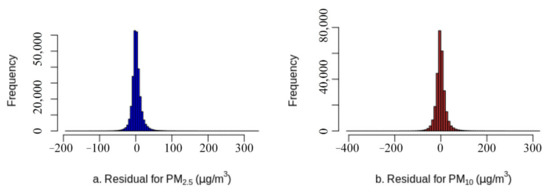
Figure 9.
Histograms of the residuals in the site-based independent testing ((a) for PM2.5; (b) for PM10).
Compared with other seven typical methods including a full residual deep network, local graph convolution network, random forest, XGBoost, regression kriging, kriging and a generalized additive model, the proposed geographic graph hybrid network improved test R2 by 5–57% for PM2.5 and 4–87% for PM10, and independent test R2 by 8–57% for PM2.5 and 8–78% for PM10; correspondingly, it decreased test RMSE by 11–49% for PM2.5 and 6–61% for PM10, and independent test RMSE by 14–46% for PM2.5 and 15–48% for PM10. Especially, although GGHN had training R2 (0.91 vs. 0.92–0.94) similar to or slightly lower than that of a full residual deep network and random forest, it had considerably better testing and independent testing R2 (0.82–0.85 vs. 0.71–0.81) and RMSE (13.87–14.51 μg/m3 vs. 15.51–17.63 μg/m3 for PM2.5; 23.54–24.34 μg/m3 vs. 24.98–30.34 μg/m3 for PM10), which indicated more improvement in generalization and extrapolation than the two methods. Compared with generalized additive model (GAM), the proposed geographic graph hybrid network achieved the maximum improvement in testing (R2 by 57% for PM2.5 and 87% for PM10) and independent testing (R2 by 57% for PM2.5 and 78% for PM10).
In addition, without the downstream network structure of the full residual deep network (Figure 3c), the local graph convolutional network only had a low performance (independent testing R2: 0.65 for PM2.5 and PM10; RMSE: 20.98 μg/m3 for PM2.5 and 33.78 μg/m3 for PM10). The downstream full residual deep network improved the performance by about 29% in testing R2 and about 26–28% in site-based independent testing R2. This showed that the downstream full residual deep network considerably reduced over-smoothing in the graph convolutional network. Without geographic graph convolutions, the full residual deep network just had a low performance (independent testing R2: 0.71–0.72). The addition of GCs improved the performance by about 4–5% in testing R2 and about 15% in site-based independent testing R2. The results showed that geographic graph convolutions made a considerable contribution to the reduction in over-fitting and the improvement in generalization for the trained model. Statistics of the performance measures of the site-based independent test showed significant difference between regions (Supplementary Table S2). In particulate, compared with the other regions, Northwest China had fewer monitoring sites with complex terrain, and lower R2 and higher RMSE.
3.3. Findings
3.3.1. Surfaces of Predicted PM2.5 and PM10 Concentration for Mainland China
Using the trained model, the daily surfaces of the predicted PM2.5 and PM10 concentrations in mainland China from 2015 to 2018 were obtained. Figure 10 shows the predicted surfaces of PM2.5, PM10 and the ratio of PM2.5 to PM10 for four typical seasonal and yearly dates: 15 April 2015 for spring, 15 July 2016 for summer, 15 October 2017 for fall and 15 December 2018 for winter.
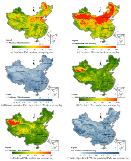
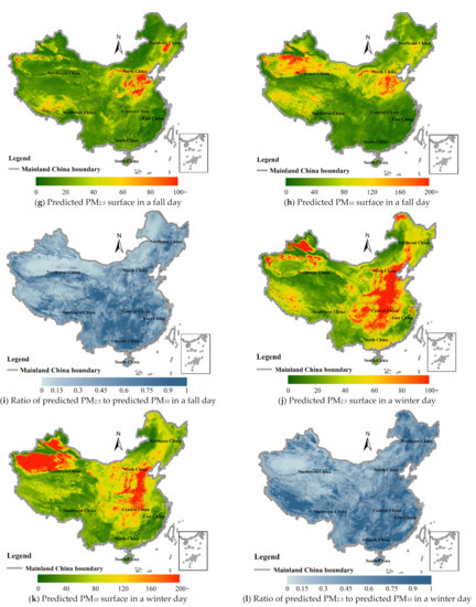
Figure 10.
Surfaces of predicted PM2.5 and PM10 (unit: μg/m3) and their ratio of PM2.5 to PM10 for four typical seasonal days ((a–c): a spring day of 15 April 2015; (d–f): a summer day of 15 July 2016; (g–i): a fall day of 15 October 2017; (j–l) for a winter day of 15 December 2018) in mainland China.
On the spring day of 15 April 2015, the northern part of mainland China experienced the largest sandstorm since 2002 [101]. Therefore, the PM10 concentration on this day was very high as shown in the predicted surface (Figure 10a,b). Compared with PM10, the concentration of PM2.5 on this day was not so high, and their high values were limited to local regions of North China, Northeast China and Northwest China. Although PM2.5 is a subset of PM10 particles, sand dust was one of the primary emission sources of PM10 in this sandstorm day, and the emission sources of PM2.5 mainly included combustion of gasoline, oil, diesel fuel and wood burning [102], etc. The surface of ratio of PM2.5 to PM10 (Figure 10c) showed low values in most locations, indicating that there was a significant difference between the two on this sandstorm day.
Different from the spring day of 2015, the summer day of 15 July 2016 (Figure 10d–f) had the lowest PM2.5 and PM10 concentration while the Taklimakan desert and its surrounding areas had higher concentrations of PM than other regions. In addition, the PM surfaces on the fall day of 15 October 2017 had low concentration (Figure 10g–i). The winter day of 15 December 2018 (Figure 10j–l) had the highest PM2.5 concentration, mostly located in Central and North China, and the local area of Urumqi. This winter day also had higher PM concentration than summer and autumn. The ratio of PM2.5 to PM10 in autumn and winter was higher than that in other seasons, indicating that many components of PM10 in these two seasons were composed of PM2.5 components.
3.3.2. Seasonal and Yearly Variation of the Predicted Surfaces
The daily and seasonal averages of predicted PM2.5 and PM10 surfaces were summarized for mainland China (Figure 11 for mean and median) and for seven geographic regions within it (Figure 12 and Figure 13). Due to the influence of extreme high values, the seasonal trend of the mean was higher than that of the median; compared with the mean, the median was more robust to the extreme high values and presented a more stable seasonal trend. In addition, PM10 showed much higher standard deviation than PM2.5 (Supplementary Figure S2). PM2.5 and PM10 showed an overall downward trend year by year, and the concentration in winter was higher than that in summer. From 2015 to 2018, the annual average concentration decreased by about 15.6% for PM2.5 and by 8.9% for PM10. The ratio of PM2.5 to PM10 decreased by about 5.4%, indicating that the decrease in PM2.5 contributed more to the air pollution caused by particulate matters. The results were consistent with the focus of the “declare war on pollution” policy of the government of China [103,104], which was to reduce PM2.5 concentration.
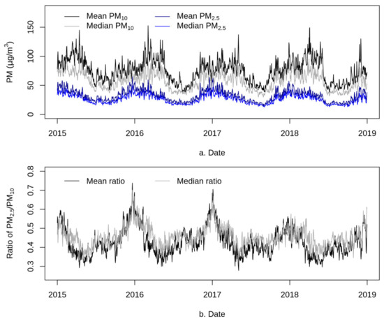
Figure 11.
Time series plots of the means of predicted PM2.5 and PM10 concentrations (a) and their ratio (b) across mainland China.
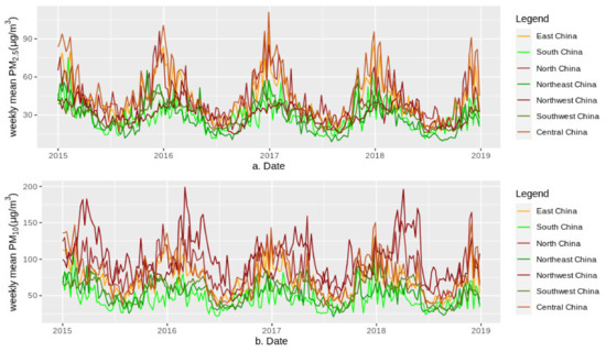
Figure 12.
Weekly means of predicted PM2.5 (a) and PM10 (b) concentrations from 2015 to 2018 for seven geographical regions in mainland China.
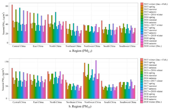
Figure 13.
Seasonal means of predicted PM2.5 (a) and PM10 (b) concentrations from 2015 to 2018 for seven geographical regions in mainland China.
The pollution level of PM2.5 was highest in central China, followed by eastern and northern China, as shown by seasonal changes (Figure 12 and Figure 13). The pollution level of PM10 was highest in northwestern China, followed by northern and central China. Southern and southwestern China had the lowest levels of PM2.5 and PM10. Compared with the central, eastern and northern regions of mainland China, although the PM2.5 pollution level in northwestern China was lower, its pollution level of PM10 was the highest due to the impact of sand dust from the Taklimakan Desert, which was one of the main components of PM10 in this area. The emission sources of PM2.5 contained the combustion of gasoline, oil, diesel and wood burning, etc., in the developed regions such as central, eastern and northern China, leading to higher levels of PM2.5 in these regions compared to the other, less-developed regions. In addition, seasonal statistics (Figure 13) showed that compared with other regions with low PM2.5, the PM2.5 decline in central, eastern, northern and northeastern China was more pronounced, and the PM10 decline in central, eastern and northwestern China was more pronounced. Due to the impact of sandstorms from Mongolia, the decrease in PM10 in northern China was relatively small compared to that in PM2.5.
3.3.3. Local Variation in the Predicted Surfaces
Figure 14 shows the enlarged grid surfaces of predicted PM2.5 and PM10 for four typical seasonal days and four representative regions: a spring day for the Jingjintang metropolitan area (a,b), a summer day for the surrounding area of Urumqi (c,d), a fall day for the Pearl River Delta (e,f) and a winter day for the Yangtze River Delta (g,h).
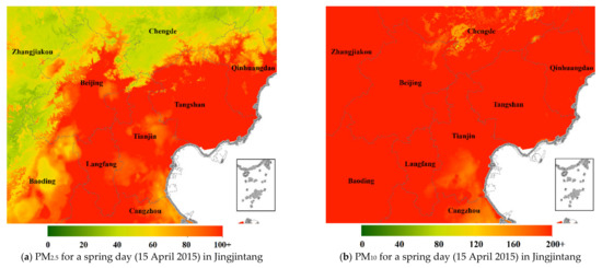

Figure 14.
Predicted surfaces of PM2.5 and PM10 for four typical seasonal days in four typical regions ((a,b) for the Jinjintang metropolitan area; (c,d) for the Urumqi city and its surroundings; (e,f) for Pearl River Delta; (g,h) for Yangtze River Delta).
These enlarged 1 × 1 km2 daily surfaces of predicted pollutants clearly showed spatial distribution of PM2.5 and PM10 concentrations and significant difference between the two. For the Jingjintang region, the PM10 level in the whole area was high but the PM2.5 pollution in the northwest area was low in the sandstorm day of 2015; the desert area of Xinjiang had a higher pollution level of PM than the other regions in the summer day of 2016; the Pearl River Delta had less PM pollution than other regions in the fall day of 2017; the Yangtze River Delta had more PM2.5 pollution than PM10 in the winter of 2018.
4. Discussion
This paper proposes a powerful deep learning method of a geographic graph hybrid network to model the neighborhood feature to improve the generalization and extrapolation accuracy of PM2.5 and PM10. Using Tobler’s First Law of Geography and local graph convolutions, the flexible hybrid framework was constructed based on spatial or spatiotemporal distances. Through powerful semi-supervised weighted embedded learning of graph convolutions, the neighborhood feature was learned from multilevel neighbors. Compared with seven representative methods, our geographic graph hybrid method substantially improved the generalization in R2 by about 8–57% for PM2.5 and 8–78% for PM10, as shown in the site-based independent test. Compared with the transductive graph network, the proposed method modeled the spatial neighborhood feature by a local inductive network structure, and thus was more generable for new samples unseen by the trained model. Compared with the-state-of-the-art methods such as random forest, XGBoost and full residual deep network, the proposed method achieved better generalization although their training performances were pretty similar. Compared with other deep learning methods, the stable learning processes of testing and site-based testing tend to converge as the index of learning epochs increases, and the fluctuations are small, indicating that the generalization has been improved. For remote areas in the study area, such as the northwestern region, compared with the other areas, there were fewer monitoring sites with complex terrain, and the site-based test performance was slightly lower, and the proposed method still worked. As far as we know, this is one of the first studies to propose the geographic graph hybrid network to improve the generalization and extrapolation of the trained model for PM2.5 and PM10.
With the strong learning ability supported by automatic differentiation and embedded learning, the proposed geographic graph hybrid network has the ability to approximate arbitrary nonlinear functions [105]. Compared with traditional spatial interpolation methods such as kriging and regression kriging, it better captured spatial or spatiotemporal correlation, without the need to satisfy the assumptions of second-order stationarity and spatial homogeneity [39,106], therefore substantially improving the generalization by about 15–51% in R2 for PM2.5 and about 17–49% in R2 for PM10. Sensitivity analysis showed that three levels of graph convolutions with 12 nearest neighbors had an optimal solution for spatiotemporal neighborhood modeling of PM. The reduction in graph convolutions and/or the number of nearest neighbors reduced the generalization of the trained model. Although a further increase in graph convolutions can further improve the generalization ability of the trained model, this improvement is trivial for PM modeling and requires more intensive computing resources. This showed that compared with neighbors that were closer to the target geo-features, the remote neighbors beyond a certain range of spatial or spatiotemporal distance had limited impact on spatial or spatiotemporal neighborhood modeling.
As the results showed, although the full residual deep network had a performance similar to the proposed geographic graph method, it performed poorer than the proposed method in regular testing and site-based independent testing. In addition, there were considerable differences (≥10%) in the performance between the independent test and test (R2 increased by about 4–5% vs. 15%; RMSE decreased by about 6–10% vs. 18–20%). This showed that the site-based independent test measured the generalization and extrapolation capability of the trained model better than the regular validation test. Sensitivity analysis also showed that the geographic graph model performed better than the nongeographic model in which all the features were used to derive the nearest neighbors and their distances. This showed that for geo-features such as PM2.5 and PM10 with strong spatial or spatiotemporal correlation, it was appropriate to use Tobler’s First Law of Geography to construct a geographic graph hybrid network, and its generalization was better than general graph networks.
Compared with decision tree-based learners such as random forest and XGBoost, the proposed geographic graph method did not require discretization of input covariates [55], and maintained a full range of values of the input data, thereby avoiding information loss and bias caused by discretization. In addition, tree-based learners lacked the neighborhood modeling by graph convolution. Although the performance of random forest in training was pretty similar to the proposed method, its generalization was worse compared with the proposed method, as shown in the site-based independent test.
Compared with the pure graph network, the connection with the full residual deep layers is crucial to reduce over-smoothing in graph neighborhood modeling. The residual connections with the output of the geographic graph convolutions can make the error information directly and effectively back-propagate to the graph convolutions to optimize the parameters of the trained model. The hybrid method also makes up for the shortcomings of the lack of spatial or spatiotemporal neighborhood feature in the full residual deep network. In addition, the introduction of geographic graph convolutions makes it possible to extract important spatial neighborhood features from the nearest unlabeled samples in a semi-supervised manner. This is especially useful when a large amount of remotely sensed or simulated data (e.g., land-use, AOD, reanalysis and geographic environment) are available but only limited measured or labeled data (e.g., PM2.5 and PM10 measurement data) are available.
For PM modeling, the physical relationship (PM2.5 ≤ PM10) between PM2.5 and PM10 was encoded in the loss through ReLU activation and RSE. Compared with a model with a single output, a model with two or more output variables (such as PM2.5 and PM10 concentrations) has the advantage that the parameters in the geographic graph model can be shared and the PM2.5-PM10 relationship can be embedded in the model. Sharing network parameters between different outputs also helps to reduce overfitting and improve generalization ability [107,108]. In particulate, the trained model can maintain a physically reasonable relationship between the output variables, which is important for the generalization and extrapolation of the trained model. Taking into account the significant differences in the emission sources and components of PM2.5 and PM10, the concentration grid surfaces predicted by the trained model presented significant differences in spatial and seasonal changes between the two, which were consistent with observational data and mechanical knowledge [109]. Sensitivity analysis showed that a model with a single output (PM2.5 or PM10 concentration) and not restricted by the PM2.5-PM10 relationship generated a few outliers with predicted PM2.5 greater than predicted PM10, indicating that two or more shared outputs and the relational constraint between them made an important contribution to the correct predictions.
This study has several limitations. First, the unavailability of high-resolution meteorological data in certain regions and time periods may limit the applicability of the proposed PM2.5 and PM10 inversion method. However, based on the publicly shared measurement data of meteorological monitoring stations and coarse-resolution reanalysis data, reliable high-resolution meteorological data can be easily inversed by using existing deep learning interpolation methods [85,86]. In addition, the other high-resolution meteorological dataset can alternatively be used for the proposed method. For example, the Gridded Surface Meteorological (gridMET) Dataset [110] can be used to estimate PM2.5 and PM10 concentrations for contiguous U.S. Second, the proposed method only estimated the total concentrations of PM2.5 and PM10, which was limited for accurately identifying the health risks of PM pollutants. The compositions and sizes of PM are different in different countries and regions, with different toxicity and health effects [102]. Accurate estimation of the hazardous components of the PM pollutants is important for downstream assessment of their health effects, and pollution prevention and control. However, considering the lack of expensive measurement data of PM constituents and their high regional variability, the inversion of PM compositions is really challenging. Third, although a total of 20 geographic graph hybrid networks were trained to obtain average performance, the training model had no uncertainty estimation, which was one of the limitations of this study.
In terms of future prospects, an extension of this research is to adapt the proposed method to effectively predict the most hazardous constituents of PM, in a semi-supervised manner, when only limited measurement data of PM constituents are available. Thereby the health risk of PM pollutants can be more accurately identified. Another future extension is uncertainty estimation, which is important as it can be provided as useful information for downstream applications. For the proposed method, the nonparametric bootstrapping method can be used to estimate the prediction error as an uncertainty measure. This method performs similarly to the parametric one, but it is widely used for various applications, including non-normal noise and nonlinear data, such as PM estimation.
5. Conclusions
This study presents a novel deep geometric learning method that combines a geographic graph network and a full residual deep network for robust spatial or spatiotemporal prediction of PM2.5 and PM10. According to Tobler’s First Law of Geography and local graph convolutions, compared with nongeographic models, the geographic graph hybrid network is constructed to be flexible, inducive and generalizable. The spatial or spatiotemporal neighborhood feature is encoded by local multilevel graph convolutions and extracted from the surrounding nearest sensed data from satellite and/or UAVs. Limited measured or labeled data of the dependent (target) variable(s) are then used to drive adaptive learning of the geographic graph hybrid model. The physical PM2.5–PM10 relationship is also encoded in the loss function to decrease over-fitting and intractable bias in the prediction. In the national forecast of PM2.5 and PM10 in mainland China, compared with seven representative methods, the presented method considerably improves R2 by 8–87% and reduces RMSE by 14–48% in site-based independent tests. With high R2 of 0.82–0.83 in the independent test, the geographic graph hybrid method created the inversion of PM2.5 and PM10 at the high spatial (1 × 1km2) and temporal resolution (daily), which was consistent with observed spatiotemporal trends and patterns. This study has important implications for high-accuracy and high-resolution robust inversions of geo-features with strong spatial or spatiotemporal correlation such as air pollutants of PM2.5 and PM10.
Supplementary Materials
The following are available online at https://www.mdpi.com/article/10.3390/rs13214341/s1: Figure S1: Bar plots of SHAP values of the trained model (a for PM2.5 and b for PM10); Figure S2: Time series plots of the standard deviations of predicted PM2.5 and PM10 concentrations across mainland China; Table S1: Statistics of meteorological factors for the PM monitoring sites; Table S2: Statistics of the performance metrics of the site-based independent test in mainland China and its geographic regions.
Funding
This work was supported in part by the National Natural Science Foundation of China under Grant 42071369 and 41871351, and in part by the Strategic Priority Research Program of the Chinese Academy of Sciences under Grant XDA19040501.
Institutional Review Board Statement
Not applicable.
Informed Consent Statement
Not applicable.
Data Availability Statement
The sample data for mainland China can be obtained from https://github.com/lspatial/geographnetdata (accessed on 1 October 2021). The Python library of Geographic Graph Hybrid Network is publicly available at https://pypi.org/project/geographnet (accessed on 1 October 2021) or https://github.com/lspatial/geographnet (accessed on 1 October 2021).
Acknowledgments
The support of NVIDIA Corporation through the donation of the Titan Xp GPUs. The author acknowledges the contribution of Jiajie Wu for data processing.
Conflicts of Interest
The authors declare no conflict of interest.
Appendix A
Table A1.
MERRA2 and MERRA2-GMI covariates for PM modeling.
Table A1.
MERRA2 and MERRA2-GMI covariates for PM modeling.
| Class | Variable | Unit | Description and Source |
|---|---|---|---|
| PBLH | Planetary boundary layer height (PBLH) | m | From NASA GMI. |
| MERRA2-GMI | Carbon monoxide | mol mol−1 | Bottom layer diagnostics (50–60 m above the ground): hourly values for a variety of surface-level values, including PM, PM2.5, NO and NO2. These will likely provide the most valuable model inputs. |
| Dust mass mixing ratio PM2.5 | kg kg−1 | ||
| Nitrate mass mixing ratio | kg/kg | ||
| Nitrogen dioxide | mol mol−1 | ||
| Ozone | mol mol−1 | ||
| Organic carbon mass mixing ratio | kg kg−1 | ||
| Total reconstructed PM2.5 | kg m−3 | ||
| Sea salt mass mixing ratio PM2.5 | kg kg−1 | ||
| Black carbon surface mass concentration | kg m−3 | Aerosol diagnostics: total aerosol extinction on an hourly basis, which may be used for model input (and estimates of surface mass concentrations for black carbon, dust, etc.). | |
| DMS surface mass concentration | kg m−3 | ||
| Dust surface mass concentration—PM2.5 | kg m−3 | ||
| Nitric acid surface mass concentration | kg m−3 | ||
| Nitrate surface mass concentration | kg m−3 | ||
| Organic carbon surface mass concentration | kg m−3 | ||
| Total reconstructed PM2.5 | kg m−3 | ||
| SO2 surface mass concentration | kg m−3 | ||
| Sea salt surface mass concentration PM 2.5 | kg m−3 | ||
| Total aerosol extinction AOT [550 nm] | - | ||
| Sulfur dioxide local | mol mol−1 | Daily satellite overpass fields: instantaneous measurements at 10 AM and 2 PM local time. | |
| Nitrogen dioxide local | mol mol−1 | ||
| 50 m eastward wind; 10 m eastward wind; 2 m eastward wind; 50 m northward wind; 10 m northward wind; 2 m northward wind | m s−1 | Single-level diagnostics: basic meteorological information such as temperature and humidity at 2 m and 10 m. These may be useful model inputs. | |
| total tropospheric ozone | Dobsons | ||
| Derived wind variables | Stagnation of wind speed, derived from wind speeds of single-level diagnostics. | m/s | |
| Wind mechanical mixing, derived from wind speeds of single-level diagnostics. | m/s |
References
- WHO. Health Effects of Particulate Matter: Policy Implications for Countries in Eastern Europe, Caucasus and Central Asia; WHO: Geneva, Switzerland, 2013. [Google Scholar]
- Dawson, J.P.; Adams, P.J.; Pandis, S.N. Sensitivity of PM2.5 to climate in the Eastern US: A modeling case study. Atmos. Chem. Phys. Discuss. 2007, 7, 4295–4309. [Google Scholar] [CrossRef]
- Hong, C.; Zhang, Q.; Zhang, Y.; Davis, S.J.; Tong, D.; Zheng, Y.; Liu, Z.; Guan, D.; He, K.; Schellnhuber, H.J. Impacts of climate change on future air quality and human health in China. Proc. Natl. Acad. Sci. USA 2019, 116, 17193–17200. [Google Scholar] [CrossRef] [PubMed]
- IASS. Air Pollution and Climate Change. Available online: https://www.iass-potsdam.de/en/output/dossiers/air-pollution-and-climate-change (accessed on 1 March 2021).
- Kloog, I.; Ridgway, B.; Koutrakis, P.; Coull, B.A.; Schwartz, J.D. Long- and short-term exposure to PM2.5 and mortality. Epidemiology 2013, 24, 555–561. [Google Scholar] [CrossRef] [PubMed]
- Yang, Y.; Ruan, Z.; Wang, X.; Yang, Y.; Mason, T.G.; Lin, H.; Tian, L. Short-term and long-term exposures to fine particulate matter constituents and health: A systematic review and meta-analysis. Environ. Pollut. 2019, 247, 874–882. [Google Scholar] [CrossRef] [PubMed]
- Benaissa, F.; Maesano, C.N.; Alkama, R.; Annesi-Maesano, I. Short-term health impact assessment of urban PM10 in Bejaia City (Algeria). Can. Respir. J. 2016, 2016, 1–6. [Google Scholar] [CrossRef]
- Maciejewska, K. Short-term impact of PM2.5, PM10, and PMc on mortality and morbidity in the agglomeration of Warsaw, Poland. Air Qual. Atmos. Health 2020, 13, 659–672. [Google Scholar] [CrossRef]
- Zeka, A.; Zanobetti, A.; Schwartz, J. Short term effects of particulate matter on cause specific mortality: Effects of lags and modification by city characteristics. Occup. Environ. Med. 2005, 62, 718–725. [Google Scholar] [CrossRef]
- Hoek, G.; Krishnan, R.M.; Beelen, R.; Peters, A.; Ostro, B.; Brunekreef, B.; Kaufman, J.D. Long-term air pollution exposure and cardio- respiratory mortality: A review. Environ. Health 2013, 12, 43. [Google Scholar] [CrossRef]
- EPA. Air Quality and Climate Change Research. Available online: https://www.epa.gov/air-research/air-quality-and-climate-change-research (accessed on 2 July 2021).
- Zhang, G.; Rui, X.; Fan, Y. Critical review of methods to estimate PM2.5 concentrations within specified research region. ISPRS Int. J. Geo-Inform. 2018, 7, 368. [Google Scholar] [CrossRef]
- Borghi, F.; Spinazzè, A.; Campagnolo, D.; Rovelli, S.; Cattaneo, A.; Cavallo, D.M. Precision and accuracy of a direct-reading miniaturized monitor in PM2.5 exposure assessment. Sensors 2018, 18, 3089. [Google Scholar] [CrossRef]
- NASA. MODIS Atmosphere. Available online: https://modis-images.gsfc.nasa.gov/products.html (accessed on 3 September 2020).
- NASA. MODIS Grids. Available online: https://modis-land.gsfc.nasa.gov/MODLAND_grid.html (accessed on 1 June 2021).
- Lyapustin, A.; Martonchik, J.; Wang, Y.; Laszlo, I.; Korkin, S. Multiangle implementation of atmospheric correction (MAIAC): 1. Radiative transfer basis and look-up tables. J. Geophys. Res. Space Phys. 2011, 116. [Google Scholar] [CrossRef]
- Lyapustin, A.; Wang, Y. MODIS Multi-Angle Implementation of Atmospheric Correction (MAIAC) Data User’s Guide; NASA. 2016. Available online: https://lpdaac.usgs.gov/documents/110/MCD19_User_Guide_V6.pdf (accessed on 1 April 2019).
- Lyapustin, A.; Wang, Y.; Laszlo, I.; Kahn, R.; Korkin, S.; Remer, L.; Levy, R.; Reid, J.S. Multiangle implementation of atmospheric correction (MAIAC): 2. Aerosol algorithm. J. Geophys. Res. Space Phys. 2011, 116. [Google Scholar] [CrossRef]
- Lyapustin, A.; Wang, Y.; Korkin, S.; Huang, D. MODIS Collection 6 MAIAC algorithm. Atmos. Meas. Tech. 2018, 11, 5741–5765. [Google Scholar] [CrossRef]
- Mhawish, A.; Banerjee, T.; Sorek-Hamer, M.; Lyapustin, A.; Broday, D.M.; Chatfield, R. Comparison and evaluation of MODIS Multi-angle Implementation of Atmospheric Correction (MAIAC) aerosol product over South Asia. Remote. Sens. Environ. 2019, 224, 12–28. [Google Scholar] [CrossRef]
- Tao, M.; Wang, J.; Li, R.; Wang, L.; Wang, L.; Wang, Z.; Tao, J.; Che, H.; Chen, L. Performance of MODIS high-resolution MAIAC aerosol algorithm in China: Characterization and limitation. Atmos. Environ. 2019, 213, 159–169. [Google Scholar] [CrossRef]
- Chiliński, M.T.; Markowicz, K.; Kubicki, M. UAS as a support for atmospheric aerosols research: Case study. Pure Appl. Geophys. PAGEOPH 2018, 175, 3325–3342. [Google Scholar] [CrossRef]
- Mamali, D.; Marinou, E.; Sciare, J.; Pikridas, M.; Kokkalis, P.; Kottas, M.; Binietoglou, I.; Tsekeri, A.; Keleshis, C.; Engelmann, R.; et al. Vertical profiles of aerosol mass concentration derived by unmanned airborne in situ and remote sensing instruments during dust events. Atmos. Meas. Tech. 2018, 11, 2897–2910. [Google Scholar] [CrossRef]
- Pikridas, M.; Bezantakos, S.; Močnik, G.; Keleshis, C.; Brechtel, F.; Stavroulas, I.; Demetriades, G.; Antoniou, P.; Vouterakos, P.; Argyrides, M.; et al. On-flight intercomparison of three miniature aerosol absorption sensors using unmanned aerial systems (UASs). Atmos. Meas. Tech. 2019, 12, 6425–6447. [Google Scholar] [CrossRef]
- NASA. Modern-Era Retrospective Analysis for Research and Applications, Version 2. Available online: https://gmao.gsfc.nasa.gov/reanalysis/MERRA-2/ (accessed on 1 April 2020).
- Nielsen, J.E.; Pawson, S.; Molod, A.; Auer, B.; da Silva, A.M.; Douglass, A.R.; Duncan, B.; Liang, Q.; Manyin, M.; Oman, L.D.; et al. Chemical mechanisms and their applications in the Goddard Earth Observing System (GEOS) earth system model. J. Adv. Model. Earth Syst. 2017, 9, 3019–3044. [Google Scholar] [CrossRef]
- Akyurtlu, A.; Akyurtlu, J. Investitation of Fine Particulate Matter, NOx and Tropospheric Ozone Transport Around a Major Roadway; Hampton University: Hampton, VI, USA, 2013. [Google Scholar]
- Frontera, A.; Martin, C.; Vlachos, K.; Sgubin, G. Regional air pollution persistence links to COVID-19 infection zoning. J. Infect. 2020, 81, 318–356. [Google Scholar] [CrossRef]
- Li, M.; Wang, L.; Liu, J.; Gao, W.; Song, T.; Sun, Y.; Li, L.; Li, X.; Wang, Y.; Liu, L.; et al. Exploring the regional pollution characteristics and meteorological formation mechanism of PM2.5 in North China during 2013–2017. Environ. Int. 2020, 134, 105283. [Google Scholar] [CrossRef]
- Benson, P. CALINE4—A Dispersion Model for Predicting Air Pollutant Concentrations Near Roadways; California Department of Transportation: Sacramento CA, USA, 1989.
- Bey, I.; Jacob, D.J.; Yantosca, R.; Logan, J.A.; Field, B.D.; Fiore, A.M.; Li, Q.; Liu, H.Y.; Mickley, L.J.; Schultz, M. Global modeling of tropospheric chemistry with assimilated meteorology: Model description and evaluation. J. Geophys. Res. Space Phys. 2001, 106, 23073–23095. [Google Scholar] [CrossRef]
- Byun, D.W.; Ching, J. Science Algorithms of the EPA Models-3 Community Multiscale Air Quality (CMAQ) Modeling System; United States Environmental Protection Agency: Washington, DC, USA, 1999.
- EPA. CMAQ v5.2 Operational Guidance Document. Available online: https://github.com/USEPA/CMAQ/blob/5.2/DOCS/User_Manual/README.md (accessed on 2 July 2020).
- Quennehen, B.; Raut, J.-C.; Law, K.S.; Daskalakis, N.; Ancellet, G.; Clerbaux, C.; Kim, S.-W.; Lund, M.T.; Myhre, G.; Olivié, D.J.L.; et al. Multi-model evaluation of short-lived pollutant distributions over east Asia during summer 2008. Atmos. Chem. Phys. Discuss. 2016, 16, 10765–10792. [Google Scholar] [CrossRef]
- Appel, K.W.; Chemel, C.; Roselle, S.; Francis, X.V.; Hu, R.-M.; Sokhi, R.S.; Rao, S.; Galmarini, S. Examination of the Community Multiscale Air Quality (CMAQ) model performance over the North American and European domains. Atmos. Environ. 2012, 53, 142–155. [Google Scholar] [CrossRef]
- Butland, B.K.; Armstrong, B.; Atkinson, R.W.; Wilkinson, P.; Heal, M.R.; Doherty, R.M.; Vieno, M. Measurement error in time-series analysis: A simulation study comparing modelled and monitored data. BMC Med. Res. Methodol. 2013, 13, 136. [Google Scholar] [CrossRef]
- Strickland, M.J.; Gass, K.; Goldman, G.T.; Mulholland, J.A. Effects of ambient air pollution measurement error on health effect estimates in time-series studies: A simulation-based analysis. J. Expo. Sci. Environ. Epidemiol. 2015, 25, 160–166. [Google Scholar] [CrossRef]
- Strickland, M.J.; Hao, H.; Hu, X.; Chang, H.H.; Darrow, L.A.; Liu, Y. Pediatric emergency visits and short-term changes in pm concentrations in the U.S. State of Georgia. Environ. Health Perspect. 2016, 124, 690–696. [Google Scholar] [CrossRef]
- Cressie, N. The origins of kriging. Math. Geol. 1990, 22, 239–252. [Google Scholar] [CrossRef]
- Gribov, A.; Krivoruchko, K. Empirical Bayesian kriging implementation and usage. Sci. Total Environ. 2020, 722, 137290. [Google Scholar] [CrossRef]
- Goovaerts, P. Geostatistics for Natural Resources Evaluation; Oxford University Press: Oxford, UK, 1997. [Google Scholar]
- Goovaerts, P. Ordinary cokriging revisited. Math. Geol. 1998, 30, 21–42. [Google Scholar] [CrossRef]
- Chu, Y.; Liu, Y.; Li, X.; Liu, Z.; Lu, H.; Lu, Y.; Mao, Z.; Chen, X.; Li, N.; Ren, M.; et al. A review on predicting ground PM2.5 concentration using satellite aerosol optical depth. Atmosphere 2016, 7, 129. [Google Scholar] [CrossRef]
- Hoek, G.; Beelen, R.; de Hoogh, K.; Vienneau, D.; Gulliver, J.; Fischer, P. A review of land-use regression models to assess spatial variation of outdoor air pollution. Atmos. Environ. 2008, 42, 7561–7578. [Google Scholar] [CrossRef]
- Lin, Y.; Zou, J.; Yang, W.; Li, C.-Q. A review of recent advances in research on PM2.5 in China. Int. J. Environ. Res. Public Health 2018, 15, 438. [Google Scholar] [CrossRef]
- Pebesma, E.; Graler, B. Introduction to Spatio-Temporal Variography; University of Münster: Münster, Germany, 2021. [Google Scholar]
- Song, Y.-Z.; Yang, H.-L.; Peng, J.-H.; Song, Y.-R.; Sun, Q.; Li, Y. Estimating PM2.5 concentrations in Xi’an City using a generalized additive model with multi-source monitoring data. PLoS ONE 2015, 10, e0142149. [Google Scholar] [CrossRef] [PubMed]
- Song, W.; Jia, H.; Huang, J.; Zhang, Y. A satellite-based geographically weighted regression model for regional PM2.5 estimation over the Pearl River Delta region in China. Remote. Sens. Environ. 2014, 154, 1–7. [Google Scholar] [CrossRef]
- Van Donkelaar, A.; Martin, R.V.; Spurr, R.J.D.; Burnett, R.T. High-resolution satellite-derived PM2.5 from optimal estimation and geographically weighted regression over North America. Environ. Sci. Technol. 2015, 49, 10482–10491. [Google Scholar] [CrossRef]
- Mirzaei, M.; Bertazzon, S.; Couloigner, I.; Farjad, B.; Ngom, R. Estimation of local daily PM2.5 concentration during wildfire episodes: Integrating MODIS AOD with multivariate linear mixed effect (LME) models. Air Qual. Atmos. Health 2019, 13, 173–185. [Google Scholar] [CrossRef]
- Xie, Y.; Wang, Y.; Zhang, K.; Dong, W.; Lv, B.; Bai, Y. Daily estimation of ground-Level PM2.5 concentrations over Beijing using 3 km resolution MODIS AOD. Environ. Sci. Technol. 2015, 49, 12280–12288. [Google Scholar] [CrossRef] [PubMed]
- Ma, J.; Yu, Z.; Qu, Y.; Xu, J.; Cao, Y. Application of the XGBoost machine learning method in PM2.5 prediction: A case study of Shanghai. Aerosol Air Qual. Res. 2020, 20, 128–138. [Google Scholar] [CrossRef]
- Pan, B. Application of XGBoost algorithm in hourly PM2.5 concentration prediction. IOP Conf. Ser. Earth Environ. Sci. 2018, 113, 012127. [Google Scholar] [CrossRef]
- Hu, X.; Belle, J.H.; Meng, X.; Wildani, A.; Waller, L.A.; Strickland, M.J.; Liu, Y. Estimating PM2.5 concentrations in the conterminous United States using the random forest approach. Environ. Sci. Technol. 2017, 51, 6936–6944. [Google Scholar] [CrossRef]
- Li, L.; Fang, Y.; Wu, J.; Wang, J.; Ge, Y. Encoder–decoder full residual deep networks for robust regression and spatiotemporal estimation. IEEE Trans. Neural Networks Learn. Syst. 2021, 32, 4217–4230. [Google Scholar] [CrossRef] [PubMed]
- Spielman, D. Spectral Graph Theory. In Combinatorial Scientific Computing; Routledge: London, UK, 2012; pp. 495–524. [Google Scholar]
- Jain, A.; Liu, I.; Sarda, A.; Monino, P. Food Discovery with Uber Eats: Using Graph Learning to Power Recommendations. Available online: https://eng.uber.com/uber-eats-graph-learning/ (accessed on 1 March 2021).
- Ying, R.; He, R.; Chen, K.; Eksombatchai, P.; Hamilton, W.L.; Leskovec, J. Graph Convolutional Neural Networks for Web-Scale Recommender Systems. In Proceedings of the 24th ACM SIGKDD International Conference on Knowledge Discovery & Data Mining, London, UK, 19–23 August 2018; pp. 974–983. [Google Scholar]
- Watters, N.; Tacchetti, A.; Weber, B.; Pascanu, R.; Zoran, D. Visual Interaction Networks: Learning a Physics Simulator from Video. In Proceedings of the 31st Conference on Neural Information Processing Systems (NIPS 2017), Long Beach, CA, USA, 4–9 December 2017. [Google Scholar]
- Mirhoseini, A.; Goldie, A.; Yazgan, M.; Jiang, J. Chip placement with deep reinforcement learning. arXiv 2020, arXiv:2004.10746. [Google Scholar]
- Sarlin, P.-E.; DeTone, D.; Malisiewicz, T.; Rabinovich, A. SuperGlue: Learning Feature Matching with Graph Neural Networks. In Proceedings of the 2020 IEEE/CVF Conference on Computer Vision and Pattern Recognition (CVPR), Seattle, WA, USA, 13–19 June 2020. [Google Scholar]
- Chanussot, L.; Das, A.; Goyal, S.; Lavril, T.; Shuaibi, M.; Riviere, M.; Tran, K.; Heras-Domingo, J.; Ho, C.; Hu, W.; et al. Open catalyst 2020 (OC20) dataset and community challenges. ACS Catal. 2021, 11, 6059–6072. [Google Scholar] [CrossRef]
- Stokes, J.M.; Yang, K.; Swanson, K.; Jin, W.; Cubillos-Ruiz, A.; Donghia, N.M.; Macnair, C.R.; French, S.; Carfrae, L.A.; Bloom-Ackermann, Z.; et al. A deep learning approach to antibiotic discovery. Cell 2020, 180, 688–702. [Google Scholar] [CrossRef] [PubMed]
- Gaudelet, T.; Day, B.; Jamasb, A.; Soman, J.; Regep, C.; Liu, G.; Hayter, J.; Vickers, R.; Roberts, C.; Tang, J.; et al. Utilizing graph machine learning within drug discovery and development. arXiv 2021, arXiv:2012.05716. [Google Scholar]
- Hamilton, W.L.; Ying, R.; Leskovec, J. Inductive Representation Learning on Large Graphs. In Proceedings of the 31st International Conference on Neural Information Processing Systems 2017 (Nips 2017), Long Beach, CA, USA, 4–9 December 2017; pp. 1025–1035. [Google Scholar]
- Ge, L.; Wu, K.; Zeng, Y.; Chang, F.; Wang, Y.; Li, S. Multi-scale spatiotemporal graph convolution network for air quality prediction. Appl. Intell. 2021, 51, 3491–3505. [Google Scholar] [CrossRef]
- Qi, Y.; Li, Q.; Karimian, H.; Liu, D. A hybrid model for spatiotemporal forecasting of PM2.5 based on graph convolutional neural network and long short-term memory. Sci. Total Environ. 2019, 664, 1–10. [Google Scholar] [CrossRef]
- Abadal, S.; Jain, A.; Guirado, R.; López-Alonso, J.; Alarcón, E. Computing graph neural networks: A survey from algorithms to accelerators. ACM Comput. Surv. 2021, 54, 1–38. [Google Scholar] [CrossRef]
- China Meteorological Administration. China Climate Bulletin 2020; China Meteorological Administration: Beijing, China, 2020. (In Chinese)
- Tang, W.-J.; Yang, K.; Qin, J.; Cheng, C.C.K.; He, J. Solar radiation trend across China in recent decades: A revisit with quality-controlled data. Atmos. Chem. Phys. Discuss. 2011, 11, 393–406. [Google Scholar] [CrossRef]
- Wikipedia. China Climate. Available online: https://zh.wikipedia.org/zh-cn/%E4%B8%AD%E5%9B%BD%E6%B0%94%E5%80%99 (accessed on 10 July 2021). (In Chinese).
- Ding, Y. China Climate; Science Press: Beijing, China, 2013. (In Chinese) [Google Scholar]
- Gelaro, R.; McCarty, W.; Suárez, M.J.; Todling, R.; Molod, A.; Takacs, L.; Randles, C.A.; Darmenov, A.; Bosilovich, M.G.; Reichle, R.; et al. The Modern-Era Retrospective Analysis for Research and Applications, Version 2 (MERRA-2). J. Clim. 2017, 30, 5419–5454. [Google Scholar] [CrossRef] [PubMed]
- Yang, S.; Chen, B. Driving forces of particulate matter emissions in China. Energy Procedia 2017, 105, 4601–4606. [Google Scholar] [CrossRef]
- Yan, B.; Liu, S.; Zhao, B.; Li, X.; Fu, Q.; Jiang, G. China’s fight for clean air and human health. Environ. Sci. Technol. 2018, 52, 8063–8064. [Google Scholar] [CrossRef] [PubMed]
- Cheng, Z.; Luo, L.; Wang, S.; Wang, Y.; Sharma, S.; Shimadera, H.; Wang, X.; Bressi, M.; de Miranda, R.M.; Jiang, J.; et al. Status and characteristics of ambient PM2.5 pollution in global megacities. Environ. Int. 2016, 89–90, 212–221. [Google Scholar] [CrossRef] [PubMed]
- Wang, W.; Zhao, S.; Jiao, L.; Taylor, M.; Zhang, B.; Xu, G.; Hou, H. Estimation of PM2.5 concentrations in China using a spatial back propagation neural network. Sci. Rep. 2019, 9, 1–10. [Google Scholar] [CrossRef] [PubMed]
- Nosratabadi, A.R.; Graff, P.; Karlsson, H.; Ljungman, A.G.; Leanderson, P. Use of TEOM monitors for continuous long-term sampling of ambient particles for analysis of constituents and biological effects. Air Qual. Atmos. Health 2019, 12, 161–171. [Google Scholar] [CrossRef]
- Guo, J.-P.; Zhang, X.-Y.; Che, H.; Gong, S.-L.; An, X.; Cao, C.-X.; Guang, J.; Zhang, H.; Wang, Y.-Q.; Xue, M.; et al. Correlation between PM concentrations and aerosol optical depth in eastern China. Atmos. Environ. 2009, 43, 5876–5886. [Google Scholar] [CrossRef]
- Li, L. High-resolution mapping of aerosol optical depth and ground aerosol coefficients for mainland China. Remote. Sens. 2021, 13, 2324. [Google Scholar] [CrossRef]
- Li, L.; Franklin, M.; Girguis, M.; Lurmann, F.; Wu, J.; Pavlovic, N.; Breton, C.; Gilliland, F.; Habre, R. Spatiotemporal imputation of MAIAC AOD using deep learning with downscaling. Remote. Sens. Environ. 2020, 237, 111584. [Google Scholar] [CrossRef] [PubMed]
- Seger, C. An Investigation of Categorical Variable Encoding Techniques in Machine Learning: Binary Versus One-Hot and Feature Hashing; KTH Royal Institute of Technology: Stockholm, Sweden, 2018. [Google Scholar]
- NASA. MERRA-2 GMI. Available online: https://acd-ext.gsfc.nasa.gov/Projects/GEOSCCM/MERRA2GMI/ (accessed on 1 June 2020).
- Press, H.W.; Teukolsky, A.S.; Vetterling, T.W.; Flannery, P.B. Numerical Recipes in C: The Art of Scientific Computing, 2nd ed.; Cambridge University Press: New York, NY, USA, 1992; pp. 123–128. [Google Scholar]
- Fang, Y.; Li, L. Estimation of high-precision high-resolution meteorological factors based on machine learning. J. Geo-Inform. Sci. 2019, 21, 799–813. [Google Scholar]
- Li, L. Geographically weighted machine learning and downscaling for high-resolution spatiotemporal estimations of wind speed. Remote. Sens. 2019, 11, 1378. [Google Scholar] [CrossRef]
- Iglewicz, B.; Hoaglin, C.D. How to detect and handle outliers. In The ASQ Basic References in Quality Control: Statistical Techniques; Mykytka, F.E., Ed.; American Society for Quality: Milwaukee, WI, USA, 1993. [Google Scholar]
- Wang, X.; Dickinson, R.E.; Su, L.; Zhou, C.; Wang, K. PM2.5 pollution in China and how it has been exacerbated by terrain and meteorological conditions. Bull. Am. Meteorol. Soc. 2018, 99, 105–119. [Google Scholar] [CrossRef]
- Zhai, S.; Jacob, D.J.; Wang, X.; Shen, L.; Li, K.; Zhang, Y.; Gui, K.; Zhao, T.; Liao, H. Fine particulate matter (PM2.5) trends in China, 2013–2018: Separating contributions from anthropogenic emissions and meteorology. Atmos. Chem. Phys. Discuss. 2019, 19, 11031–11041. [Google Scholar] [CrossRef]
- Dyatmika, H.; Sambodo, K.; Budiono, M.; Hendayani, B. Noise removal using thresholding and segmentation for random noise Sentinel-1 data. IOP Conf. Ser. Earth Environ. Sci. 2017, 54, 012105. [Google Scholar] [CrossRef]
- Freedman, D.; Pisani, R.; Purves, R. Statistics: Fourth International Student Edition; W.W. Norton & Company: New York, NY, USA, 2007. [Google Scholar]
- Zhou, J.; Cui, G.; Hu, S.; Zhang, Z.; Yang, C.; Liu, Z.; Wang, L.; Li, C.; Sun, M. Graph neural networks: A review of methods and applications. AI Open 2020, 1, 57–81. [Google Scholar] [CrossRef]
- Tobler, W. On the First Law of Geography: A Reply. Ann. Assoc. Am. Geogr. 2004, 94, 304–310. [Google Scholar] [CrossRef]
- Kipf, T.; Welling, M. Semi-supervised classification with graph convolutional networks. arXiv 2016, arXiv:1609.02907. [Google Scholar]
- Chen, D.; Lin, Y.; Li, W.; Li, P.; Zhou, J.; Sun, X. Measuring and Relieving the Over-Smoothing Problem for Graph Neural Networks from the Topological View. In Proceedings of the AAAI Conference on Artificial Intelligence 2020, New York, NY, USA, 7–12 February 2020; Volume 34, pp. 3438–3445. [Google Scholar]
- Li, L.; Girguis, M.; Lurmann, F.; Pavlovic, N.; McClure, C.; Franklin, M.; Wu, J.; Oman, L.D.; Breton, C.; Gilliland, F.; et al. Ensemble-based deep learning for estimating PM2.5 over California with multisource big data including wildfire smoke. Environ. Int. 2020, 145, 106143. [Google Scholar] [CrossRef] [PubMed]
- Gong, P.; Li, X.; Zhang, W. 40-Year (1978–2017) human settlement changes in China reflected by impervious surfaces from satellite remote sensing. Sci. Bull. 2019, 64, 756–763. [Google Scholar] [CrossRef]
- Bishop, M.C. Pattern Recognition and Machine Learning; Springer: Berlin/Heidelberg, Germany, 2006. [Google Scholar]
- Lundberg, S.M. Welcome to the SHAP Documentation. Available online: https://shap.readthedocs.io/en/latest/index.html (accessed on 5 January 2021).
- Lundberg, S.M.; Lee, S.I. A Unified Approach to Interpreting Model Predictions. In Proceedings of the 31st International Conference on Neural Information Processing Systems (Nips 2017), Long Beach, CA, USA, 4–9 December 2017; pp. 4768–4777. [Google Scholar]
- Baidu. 4.15 Sandstorm in Beijing. Available online: https://baike.baidu.com/item/4%C2%B715%E5%8C%97%E4%BA%AC%E6%B2%99%E5%B0%98%E6%9A%B4 (accessed on 12 April 2021).
- Li, X.; Jin, L.; Kan, H. Air pollution: A global problem needs local fixes. Nature 2019, 570, 437–439. [Google Scholar] [CrossRef]
- Baidu. Beijing Clean Air Action Plan for 2013–2017. Available online: https://baike.baidu.com/item/%E5%8C%97%E4%BA%AC%E5%B8%822013-2017%E5%B9%B4%E6%B8%85%E6%B4%81%E7%A9%BA%E6%B0%94%E8%A1%8C%E5%8A%A8%E8%AE%A1%E5%88%92/10348277?fr=aladdin (accessed on 2 January 2021). (In Chinese).
- Pang, N.; Gao, J.; Zhu, G.; Hui, L.; Zhao, P.; Xu, Z.; Tang, W.; Chai, F. Impact of clean air action on the PM2.5 pollution in Beijing, China: Insights gained from two heating seasons measurements. Chemosphere 2021, 263, 127991. [Google Scholar] [CrossRef] [PubMed]
- Saunders, A.; Oldenburg, I.A.; Berezovskii, V.; Johnson, C.A.; Kingery, N.D.; Elliott, H.L.; Xie, T.; Gerfen, C.R.; Sabatini, B.L. A direct GABAergic output from the basal ganglia to frontal cortex. Nat. Cell Biol. 2015, 521, 85–89. [Google Scholar] [CrossRef] [PubMed]
- Montero, J.; Fernandez-Aviles, G.; Mateu, J. Spatial and Spatio-Temporl Geostatistical Modeling and Kriging; Wiler & Sons: Hoboken, NJ, USA, 2015. [Google Scholar]
- Goodfellow, I.; Bengio, Y.; Courville, A. Deep Learning; MIT Press: Cambridge, MA, USA, 2016. [Google Scholar]
- Zhang, Z.; Luo, P.; Loy, C.C.; Tang, X. Learning deep representation for face alignment with auxiliary attributes. IEEE Trans. Pattern Anal. Mach. Intell. 2016, 38, 918–930. [Google Scholar] [CrossRef] [PubMed]
- Fan, H.; Zhao, C.; Yang, Y.; Yang, X. Spatiotemporal variations of the PM2.5/PM10 ratios and its application to air pollution type classification in China. Front. Environ. Sci. 2021, 9, 218. [Google Scholar] [CrossRef]
- Abatzoglou, T.J. Development of gridded surface meteorological data for ecological applications and modelling. Int. J. Climatol. 2011, 33, 121–131. [Google Scholar] [CrossRef]
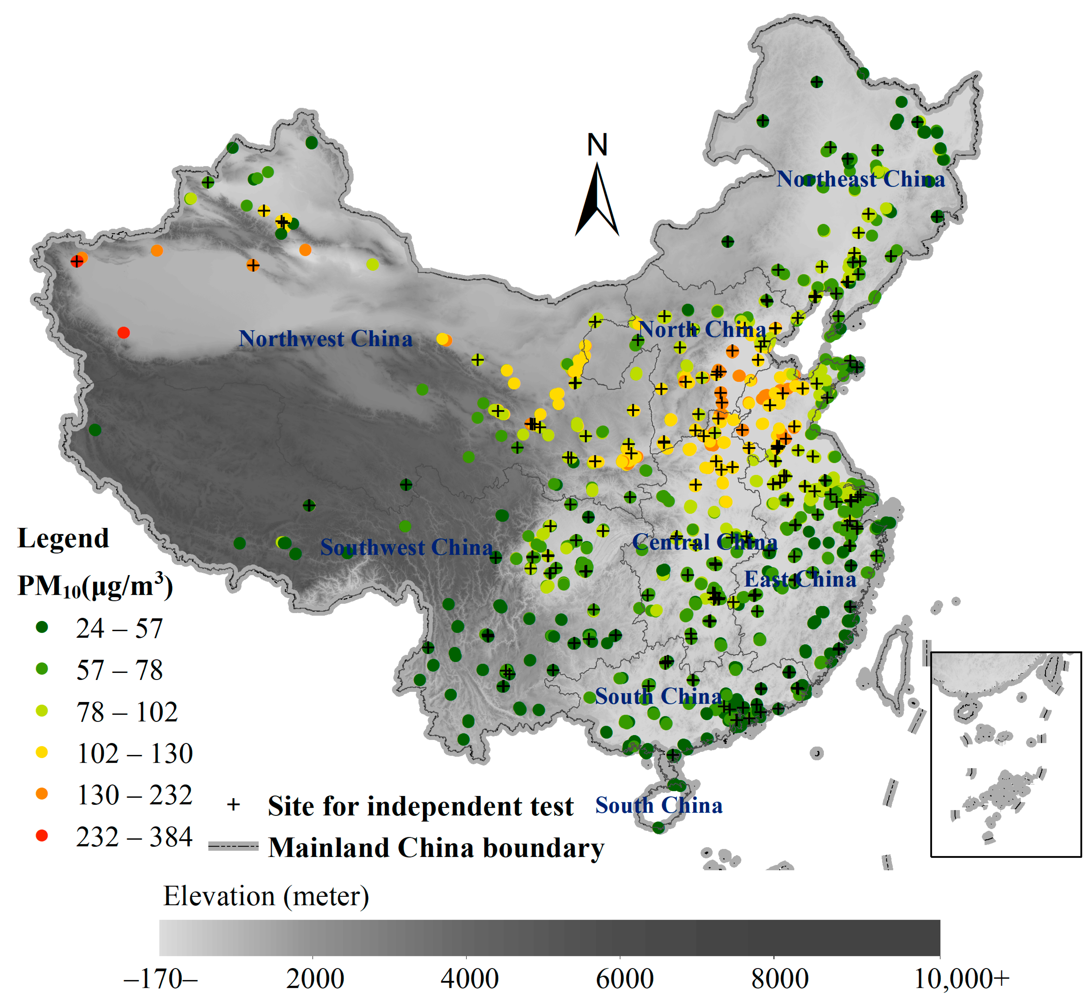

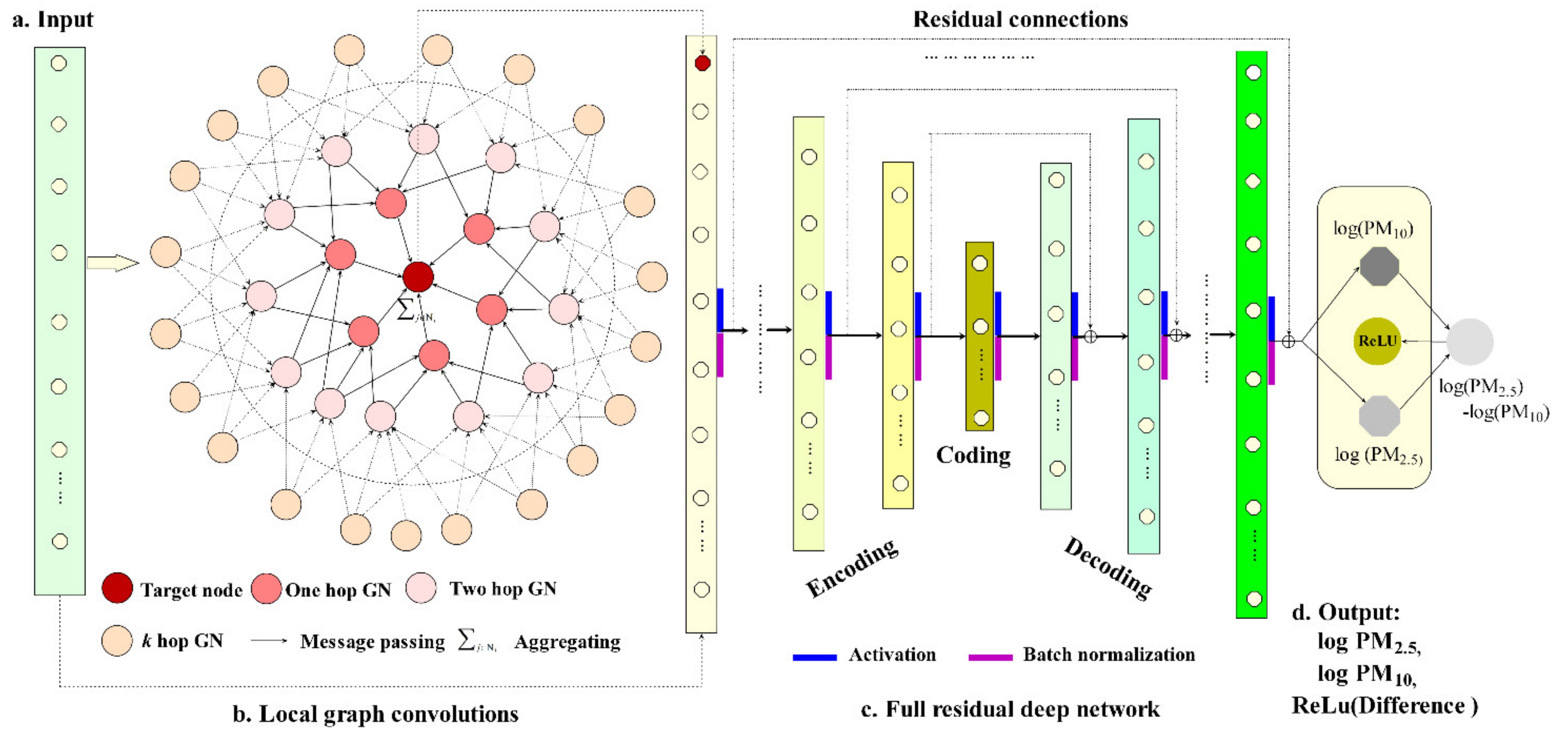

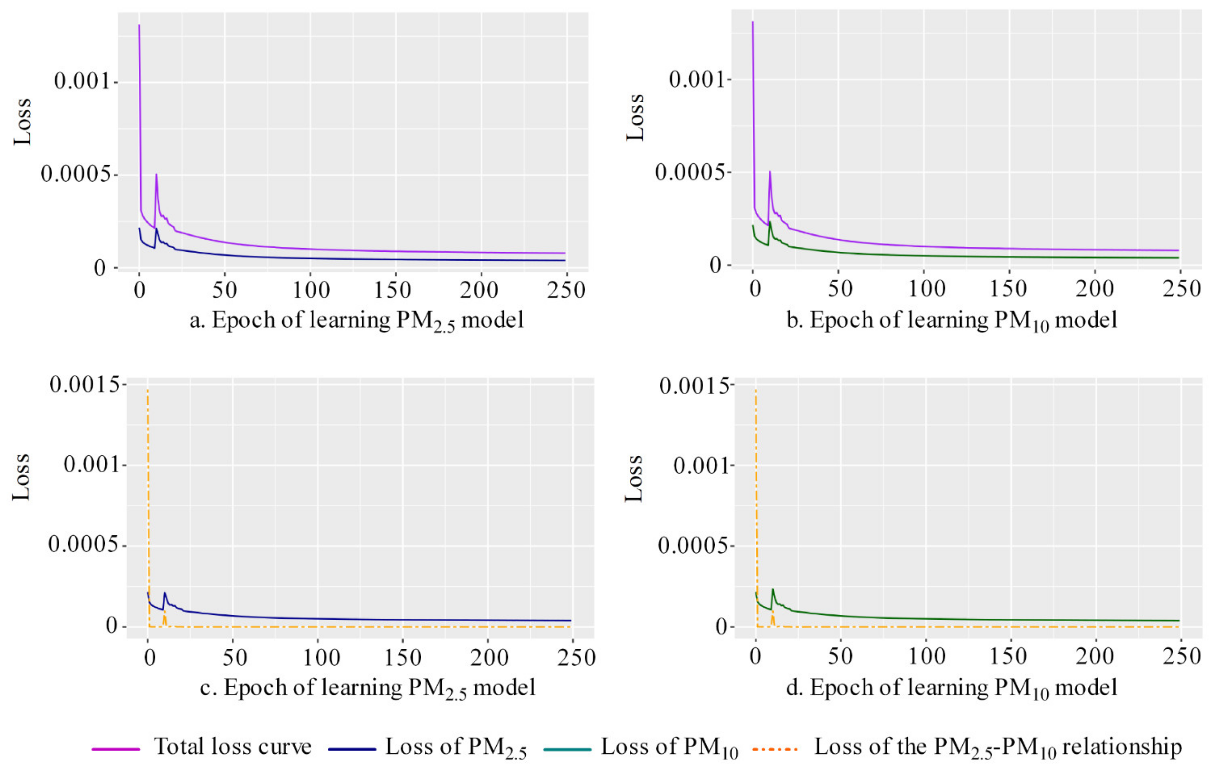
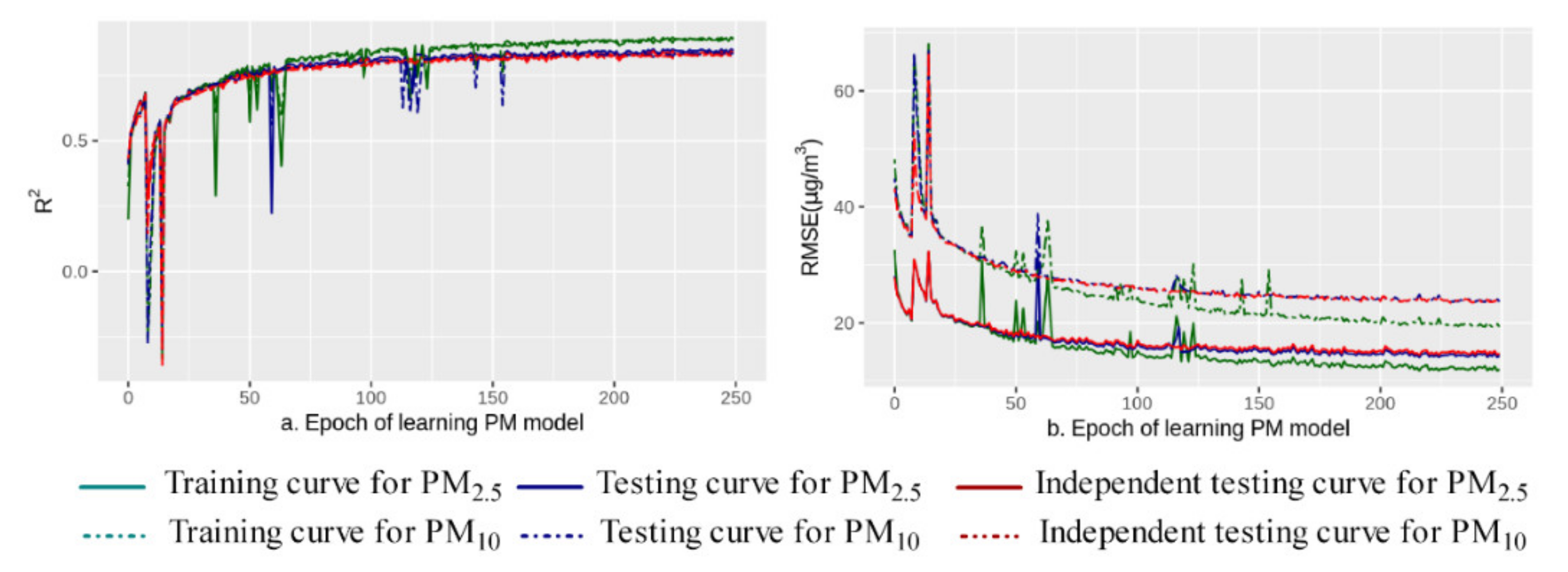
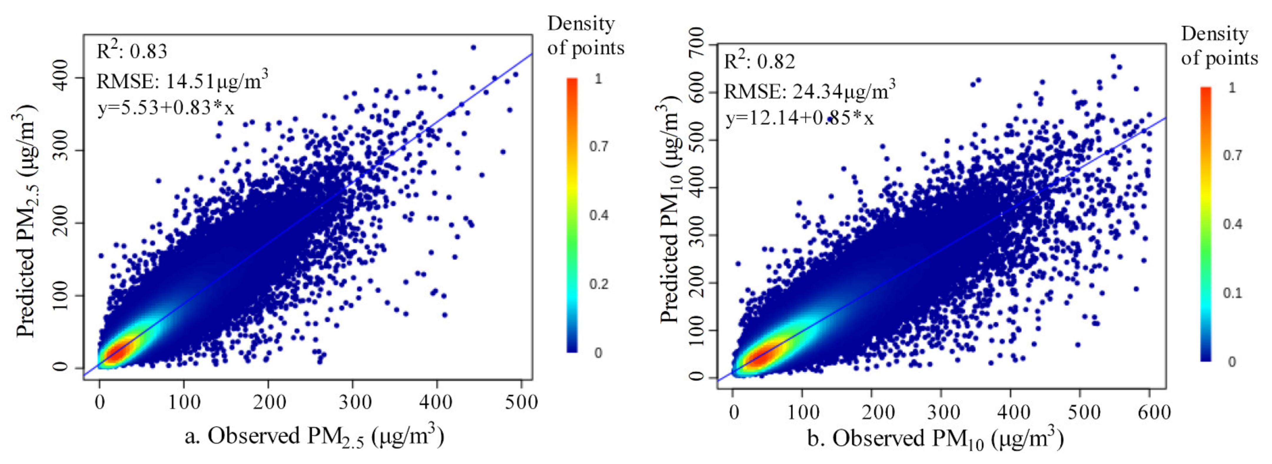
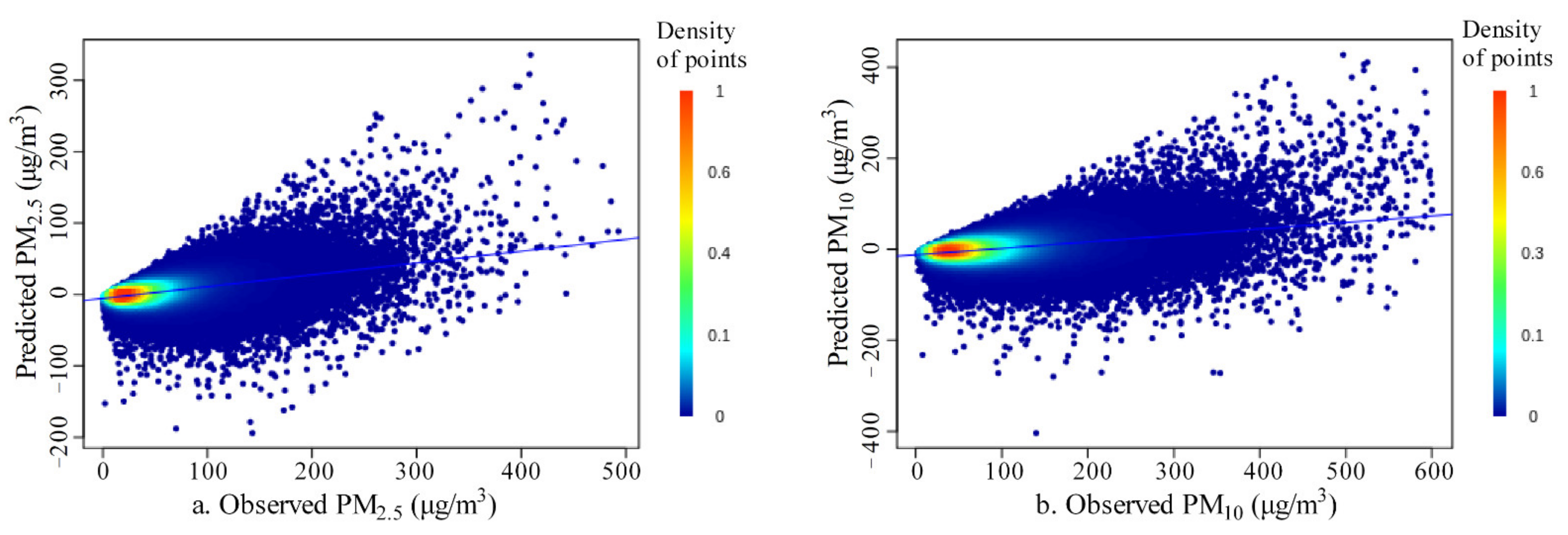

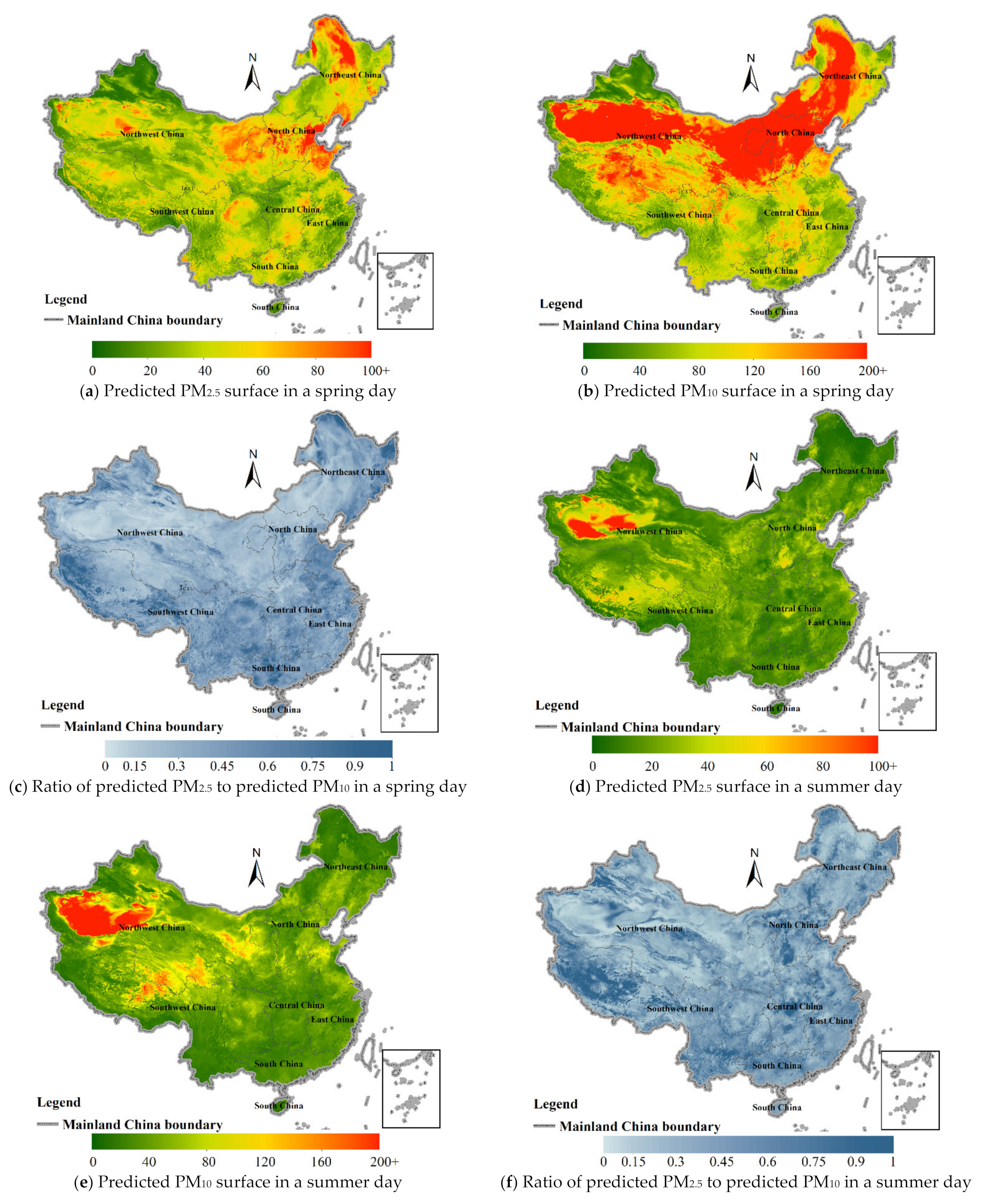


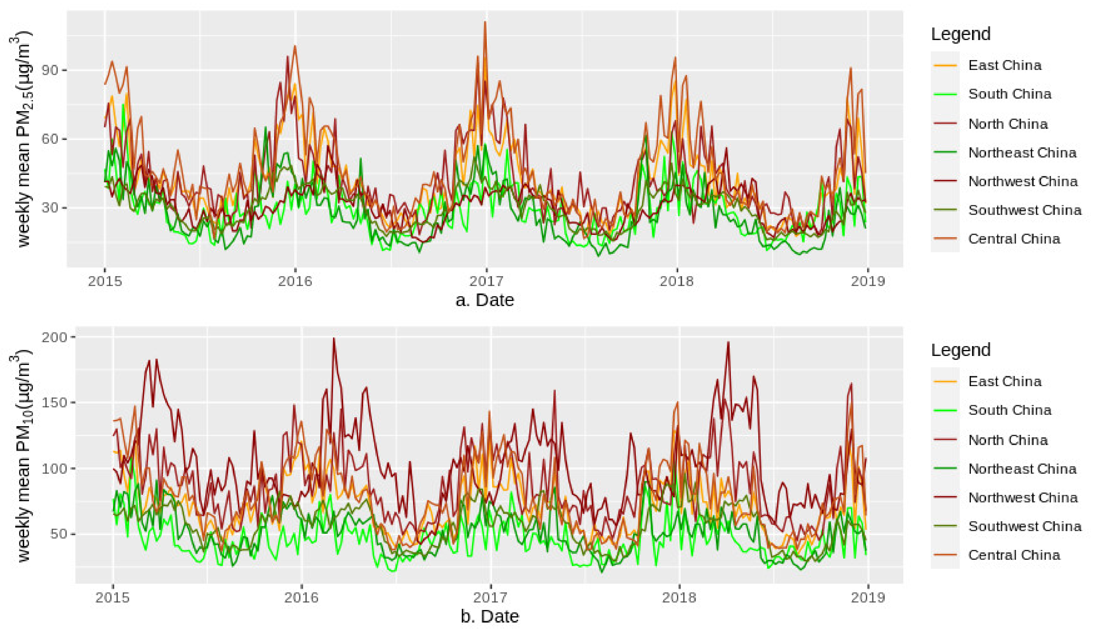

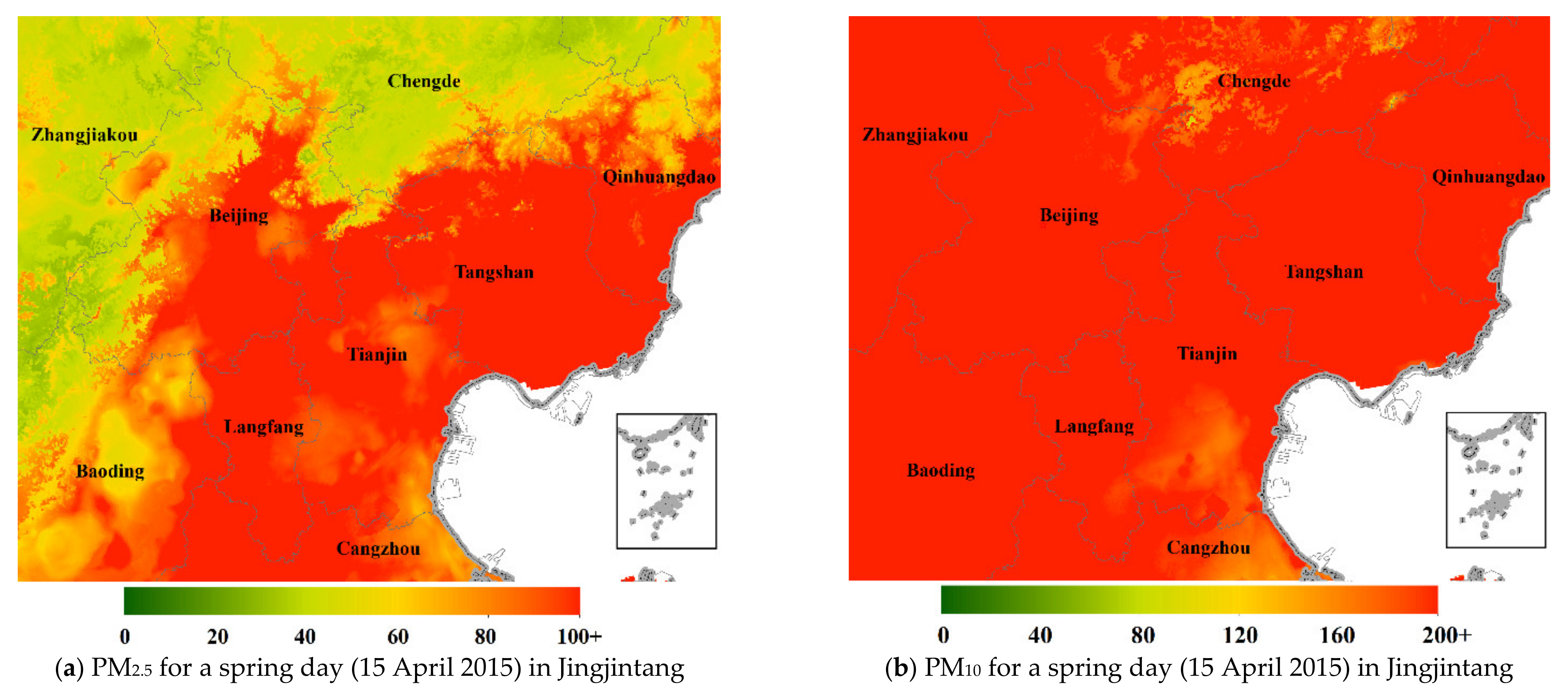
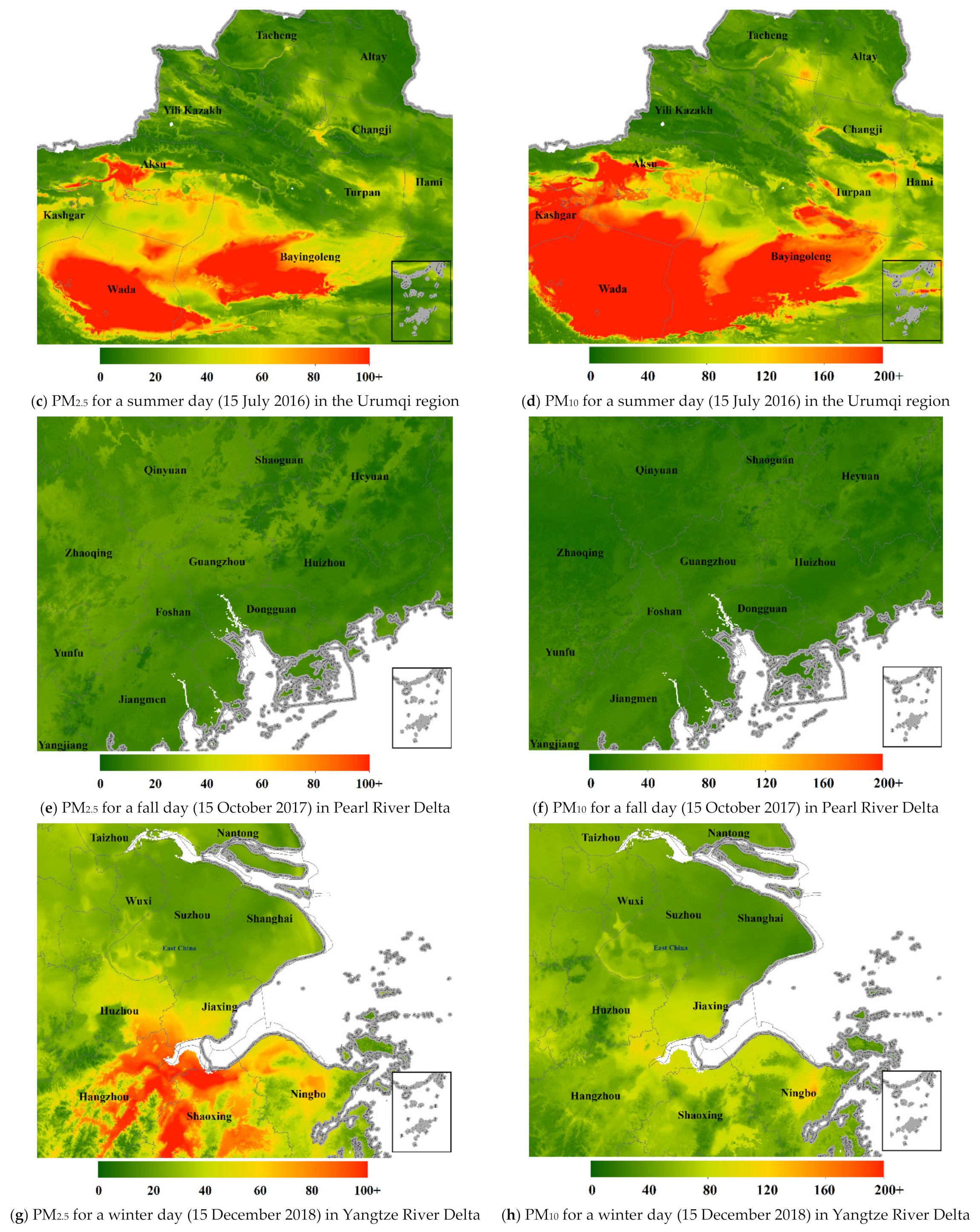
Publisher’s Note: MDPI stays neutral with regard to jurisdictional claims in published maps and institutional affiliations. |
© 2021 by the author. Licensee MDPI, Basel, Switzerland. This article is an open access article distributed under the terms and conditions of the Creative Commons Attribution (CC BY) license (https://creativecommons.org/licenses/by/4.0/).