1. Introduction
Building information extraction from Earth observation data is key to a wide range of applications, including map generation, urban sprawl monitoring, risk mapping, and urban planning. In this framework, the joint use of high resolution imagery and LiDAR data has been proposed, to produce comprehensive results by exploiting the complementary information given by the two data types. Several fusion techniques have been proposed that combine data both at the feature level [
1,
2,
3,
4,
5] and at the decision level [
6,
7]; despite the range of solutions available, however, a few unresolved issues remain. In feature-level fusion, some methods use only cross-modal features, which provide good discriminative power most of the times but fail in specific edge cases. On the other hand, individual features combined only at the decision level are often not discriminative enough to produce proper building extraction. However, they can still be useful in cases where a single data source would mislead the classifier because it contains noisy or corrupted information. Therefore, it is necessary to build a system that utilizes both individual and cross-modal features. Moreover, the fusion strategy should be such that useful discriminative features are highlighted, whereas irrelevant or noisy ones are suppressed. The Hybrid Attention-aware Fusion Network (HAFNet) [
8] offers a solution to these problems by introducing the Attention-Aware Multi-modal Fusion Block (Att-MFBlock), a computational module used to adaptively re-weight individual and cross-modal features. The proposed model achieves state-of-the-art-segmentation accuracy and provides great performance even in specific edge cases where either data type introduces noise and potentially harmful information. Consider the example in
Figure 1, where the DSM dataset suggests that the right half of the building visible on the bottom of the RGB image is not there. The information fed by the DSM dataset is clearly wrong and can negatively impact local results, but the HAFNet structure, and specifically the attention mechanism, can detect it and filter it out.
The high performance of the HAFNet model, however, comes at the cost of an enormous number of parameters. Such over-parametrization of the model conveys disadvantages both at the development level and at the deployment level, including slow training, long inference time, and massive memory footprint. All the mentioned consequences can pose problems in a time when AI applications are moving on the edge, and models are expected to work with very limited computing and memory resources.
As pointed out by researchers in Reference [
9], the reason why AI models are still confined to offline data processing is that their weights and topology are often too large to fit into the available resources onboard Earth Observation satellites. At the same time, inference of DL systems is computationally intensive, and this can be a problem in a low-power-budget environment. New networks need to be engineered taking into account the different computation restrictions related to memory usage, training, and inference time cost. On-board data processing in spaceborne Earth Observation systems is gaining relevance, and methods for different Remote Sensing applications are being developed [
9,
10,
11,
12,
13]. This trend is substantially accelerated by the recent joint effort of multiple Deep Learning research studies of providing new implementations of efficient network architectures that limit the overall number of parameters while achieving state-of-the-art performances. These networks [
14,
15,
16] are built out of custom-designed operation modules that fulfill this task.
A careful reorganization of existing architectures and introduction of efficient modules can solve the previously described problems and accelerate the transformation of AI-driven systems from offline processing tools to powerful dynamic edge applications. Motivated by these considerations, in this paper, we propose an efficient implementation of the HAFNet model called HAFNetE that exceeds state-of-the-art, fusion-based building extraction performances while, at the same time, affording a 92% reduction from the original number of network parameters. This substantial cut in requirements makes it possible to directly deploy the model as an on-board spaceborne urban mapping system.
3. HAFNet and HAFNetE
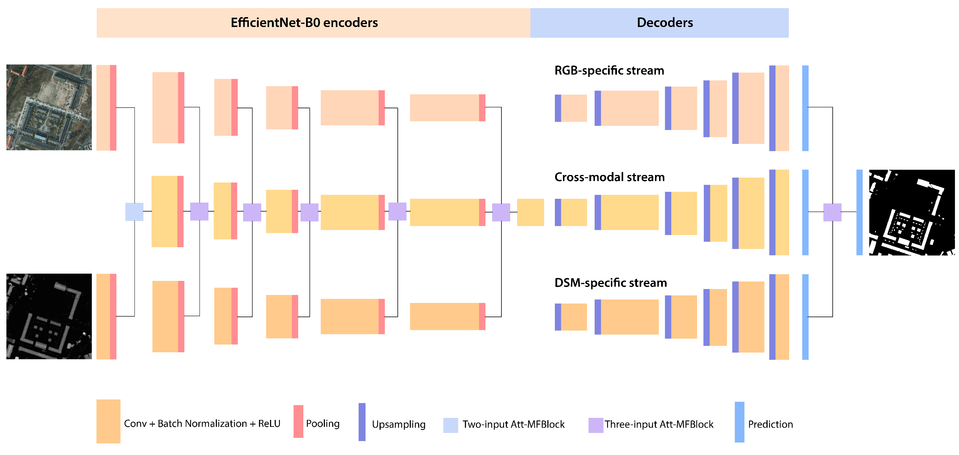
In this section, we introduce HAFNetE, an efficient hybrid attention-aware fusion network for building extraction, starting from its predecessor HAFNet or Hybrid Attention-aware Fusion Network. HAFNet is a multi-modal building extraction segmentation network that utilizes cross-modal and individual features to perform builiding footprint extraction, and it accepts HRI RGB images and LiDAR data as its inputs. The overall architecture is comprised of three streams: RGB, DSM, and cross-modal. All the streams are built as parallel SegNets [
26], where the encoder part is characterized by a VGG-16 structure. The RGB and DSM streams are designed to learn individual modal features. These features are then fused together after each set of convolutional operations with an Attention-Aware Multi-modal Fusion Block (Att-MFBlock) in the cross-modal stream. The extracted features from each stream are decoded in their respective decoder stream and finally combined at the decision stage using again an Attention-Aware Multi-modal Fusion Block to produce the final segmented output. By using both individual and cross-modal streams, it is possible to learn more discriminative features and, therefore, achieve a comprehensive building extraction result. Starting from this existing scheme, HAFNetE preserves the three-stream network concept but utilizes both a completely different single stream architecture and encoder structure. The model architecture is shown in
Figure 2.
The network is comprised of three subnetworks (streams): the RGB stream, the DSM stream, and the cross-modal stream. RGB HRI images and LiDAR-derived DSM data are fed as input to the model where features are extracted, respectively, by the RGB stream encoder and the DSM stream encoder. The extracted features are then combined in the cross-modal stream encoder by using the previously discussed Attention-aware multi-fusion block. The cross-modal specific stream is added to combine different modalities at an early stage and, therefore, to learn more discriminative cross-modal features [
27]. After the decoding phase, predictions coming from the three streams are fused using the Att-MFBlock [
8] to provide a comprehensive building extraction result. Unlike the previous HAFNet model, whose architecture was based on three parallel SegNet-like streams using VGG16-style encoders in each of them, HAFNetE introduces modifications both at the encoder level and at the single stream level. VGG-16 encoders are substituted with EfficientNet encoders. This family of models is specifically designed for good encoding performance even with limited available resources. This translates to simple networks with fewer parameters. Small models yield multiple advantages: faster training, shorter inference times, and bearable memory footprint on the system where the model is deployed. Multiple networks characterized by these features exist (MobileNet, MobileNetV2, etc.); however, an EfficientNet-B0-type encoder was selected across the candidates because it offers a good compromise in the performance/computational cost trade-off. As a matter of fact, by reducing the number of parameters in the model, performance is likely to decrease. However, EfficientNet, by scaling the number of parameters according to the Compounding Scaling method [
16], attains high performances with approximately
fewer parameters than classical models, such as ResNet-50 [
28]. An efficiency comparison between EfficientNet models and classical models is reported in
Table 1.
At the individual stream level, the SegNet structure is substituted with a U-Net network [
31]. U-Net has a similar architecture to the previously utilized SegNet and offers a suitable alternative to it, thanks to its effective feature re-localization capability. The conceptually simple architecture of U-Net makes it easy and elegant to implement. Moreover, one objective of the research is to assess whether the previously proposed HAFNet three-streams network can be generalized and effectively being employed using different base models, such as U-Net. For these reasons, U-Net was selected as the single-stream subnetwork.
To summarize, HAFNetE is a complete overhaul of the original HAFNet model. VGG16 encoders are substituted with EfficientNet encoders, and the SegNet architecture at the individual stream level is replaced with a U-Net. The only aspects retained from the previous version are the idea of combining features extracted in the HRI-RGB and LiDAR-derived DSM streams into a new cross-modal stream and the method used to fuse the encoded information. The substituted encoders and the restructured network architecture provide a completely new and, most importantly, efficient way of extracting and processing information from data. As it will be discussed thoroughly in
Section 5, even though the HAFNetE model provides an improvement at an application level in terms of segmentation capability, the most remarkable and actionable result with respect to the previously proposed HAFNet is the advanced and carefully designed, efficient architecture, that translates into a massive enhancement of computational efficiency.
A part from a few models, most of the newly proposed networks are designed to score highest in segmentation performances largely disregarding the associated computational cost. This latter can make the model impossible to use in most of real-world scenarios, where end users do not have enough computational resources, or, even if they do, the final application does not permit the use of related technologies (e.g., on-board spaceborne systems). Memory footprint, training time, and inference time are aspects that cannot be overlooked when deploying a system in production. HAFNetE is engineered taking all these details into account and with the explicit goal of making the network deployable in a on-board spaceborne system.
4. Experiment Design
4.1. Dataset
The datasets used to train and evaluate the model come from the publicly available data repository of the ISPRS 2D Semantic Labeling Challenge [
32], in the German city of Potsdam, and it is composed of high-resolution true-color orthophoto images and the corresponding normalized DSM data. The dataset also includes a smaller dataset on the German city of Vaihingen, but this part has not been included in our experiments. As it will be explained later in this paper, in terms of ortophotos, the Vaihingen dataset contributes false-color IRRG images only, whose radiometric behavior does not match what was learnt on RGB images by the pre-trained networks used in the proposed method.
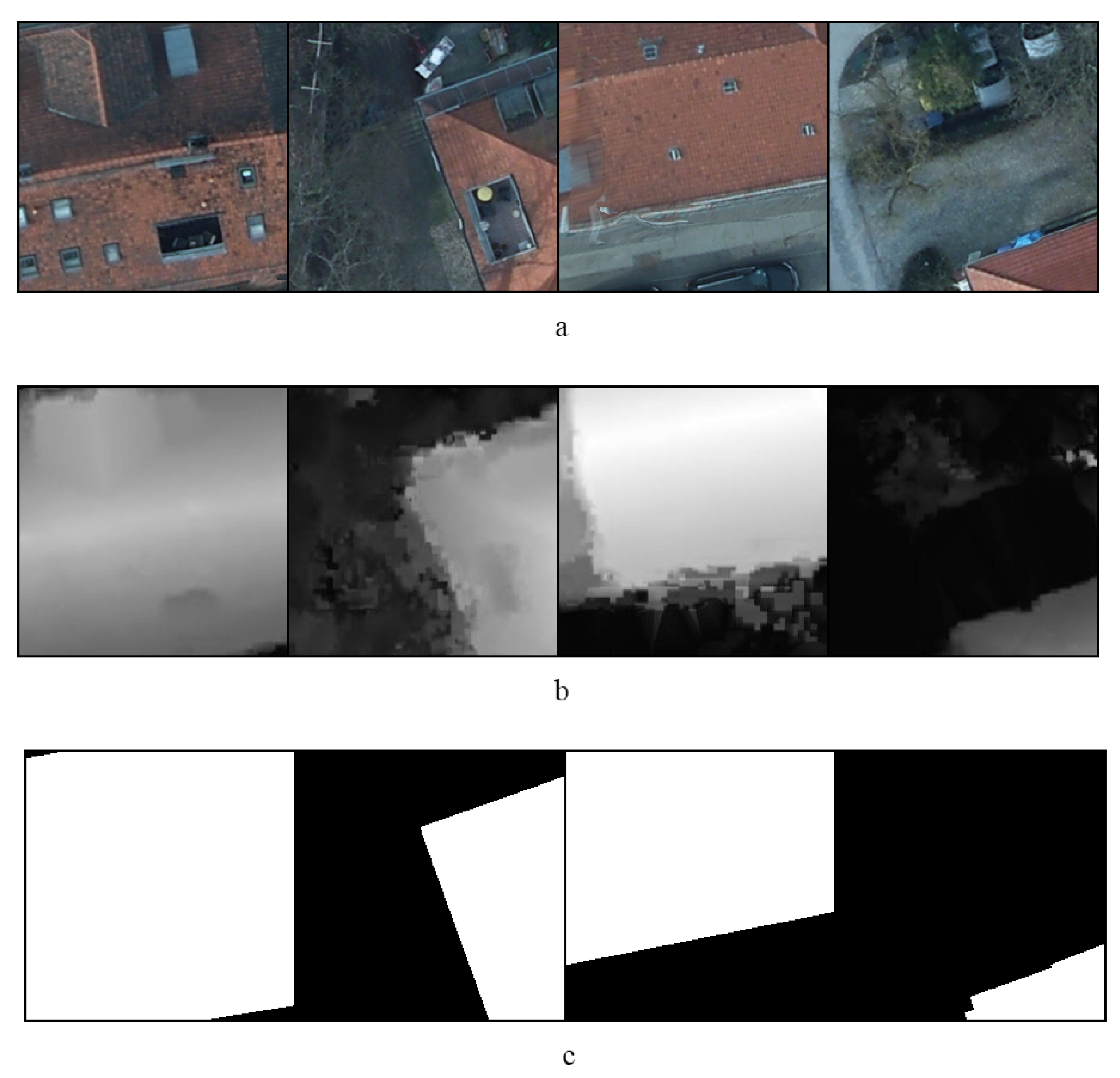
In the original dataset, each parcel of land was classified into six common land cover classes, and this classification is distributed as Ground Truth (GT) to support the supervised learning procedure. The problem addressed in this paper, i.e., basic building mapping, only uses two labels, namely “building” and “non-building”. Therefore, binary thematic maps containing only the desired classes were created by merging previous classes into the two relevant ones using simple image processing techniques. In
Figure 3, an example of an image patch with the corresponding binary thematic map is presented.
The organizers of the Challenge also defined a partition of the dataset into training and testing images. Since our research involved a Deep Learning method and, consequently, the need for hyperparameter tuning, the dataset was split into three subsets: one for training, one for validation, and one for testing. The Potsdam dataset contains 38 images that were randomly assigned to one of the three subsets so that the training subset contained ≈80%, validation ≈10%, and test ≈10% of the original images. It is to be noted that visual inspection of orthophoto images revealed noticeable geometrical distortions in some places, as in the example of
Figure 4.
These are probably due to stitching of multiple images in the production phase, and such distortions are not reflected in the ground truth, thus creating a mismatch between optical data and reference. Although the phenomenon is not very frequent across the dataset, this must be taken into account in evaluating results as it can lead to a underestimation of the actual capability of the model in segmenting the input. The model was trained using a subsection of the Potsdam dataset. The True OrtoPhoto (TOP) in such dataset come as TIFF files in different channel compositions, namely IRRG, RGB, and RGBIR. Since the model was initialized with pre-trained EfficientNet-B0 weights tuned on RGB-coded images, the RGB version of the TOP images offered in the Potsdam dataset was used. On the other hand, the Vaihingen dataset provides only IRRG TOP images; because of this mismatch, only the Potsdam section of the ISPRS 2D Semantic Labeling Challenge was used to train, validate, and test the model. It should be noted that, in any case, the Potsdam dataset contains most of the images of the entire ISPRS dataset, and, because of its dimensions in terms of number of images and single image size, the data covers a great range of variability and diverse edge cases that make the sole Potsdam section suitable for the standard training, validation, and testing Deep Learning model procedure.
4.2. Model Performance Metrics
For sake of completeness, various standard metrics were used to evaluate the model performance, namely the overall accuracy (OA), the F1 score, and the intersection over union (IoU). For the readers’ convenience, the definition of the first three metrics are reported below.
In the expressions above,
tp,
fp,
fn refer to the number of true positive, false positive, and false negative cases, respectively. The IoU metric is defined as:
Here, target represents the set of building pixels from the ground truth, and detected represents the set of pixels assigned to class “building” by the classifier. It is important to note that the number of building pixels is about one order of magnitude smaller than non-building pixels in the average considered image patch. In a segmentation setting with strong class imbalance, IoU is probably slightly more representative than the other measures, since it gauges the overlap rate of the detected target pixels and the labeled target pixels.
4.3. Training Procedure
4.3.1. Data Processing
The Potsdam dataset contains images the size of
pixels, too big to fit entirely into the GPU memory; thus, they were partitioned into multiple non-overlapping
tiles. This latter is the size of images in the ImageNet dataset [
29] and was indeed selected to maximize the encoding capabilities of the RGB and DSM encoders that were pre-trained on such standard dataset. However, this setting is not binding, and the model is flexible on the size of the input images. As previously noted, the dataset is extremely unbalanced, and most of the patches extracted from the images do not contain any building pixel. By training the model on this dataset, the net will be biased towards the non-building class, and, in the evaluation phase, the performance metrics may stay high simply because the model is most of the time correctly predicting that the examined patch does not contain buildings. Thus, a data-balancing strategy is required to avoid the network to settle on a fairly high accuracy by simply ignoring the comparatively few building pixels altogether, which results into a useless trained network. Two different approaches can be used to tackle the problem. The first method implies using a weighted loss function during training (e.g., Weighted Binary Cross Entropy) that assigns a larger weight to samples containing buildings and, therefore, induces stronger changes in the net parameters when a building is being processed. The second method [
33] suggests training the model only on positive examples, i.e., patches containing more than a pre-set number or percentage of building pixels in our case. This second approach was selected because it is expected not to affect the generalization capabilities of the network. The method was implemented by filtering the extracted patches so that only patches containing at least 5% of positive pixels (building pixels) survived. In the end, the number of effective training patches was 8800.
4.3.2. Model Training
The proposed HAFNetE was implemented using the PyTorch framework and following the design patterns of the PyTorch library Segmentation Models PyTorch (SMP) [
34]. Training and evaluation phases were conducted using a NVIDIA GeForce RTX 1080Ti GPU (11 GB memory). Since data had been previously balanced during the preprocessing phase, a simple non-weighted version of Binary Cross Entropy loss was used. Multiple experiments were carried out to choose the best optimizer for minimizing the loss function (Stochastic Gradient Descent (SGD), Adagrad, Adam).
Table 2 shows validation metrics using the different optimization strategies.
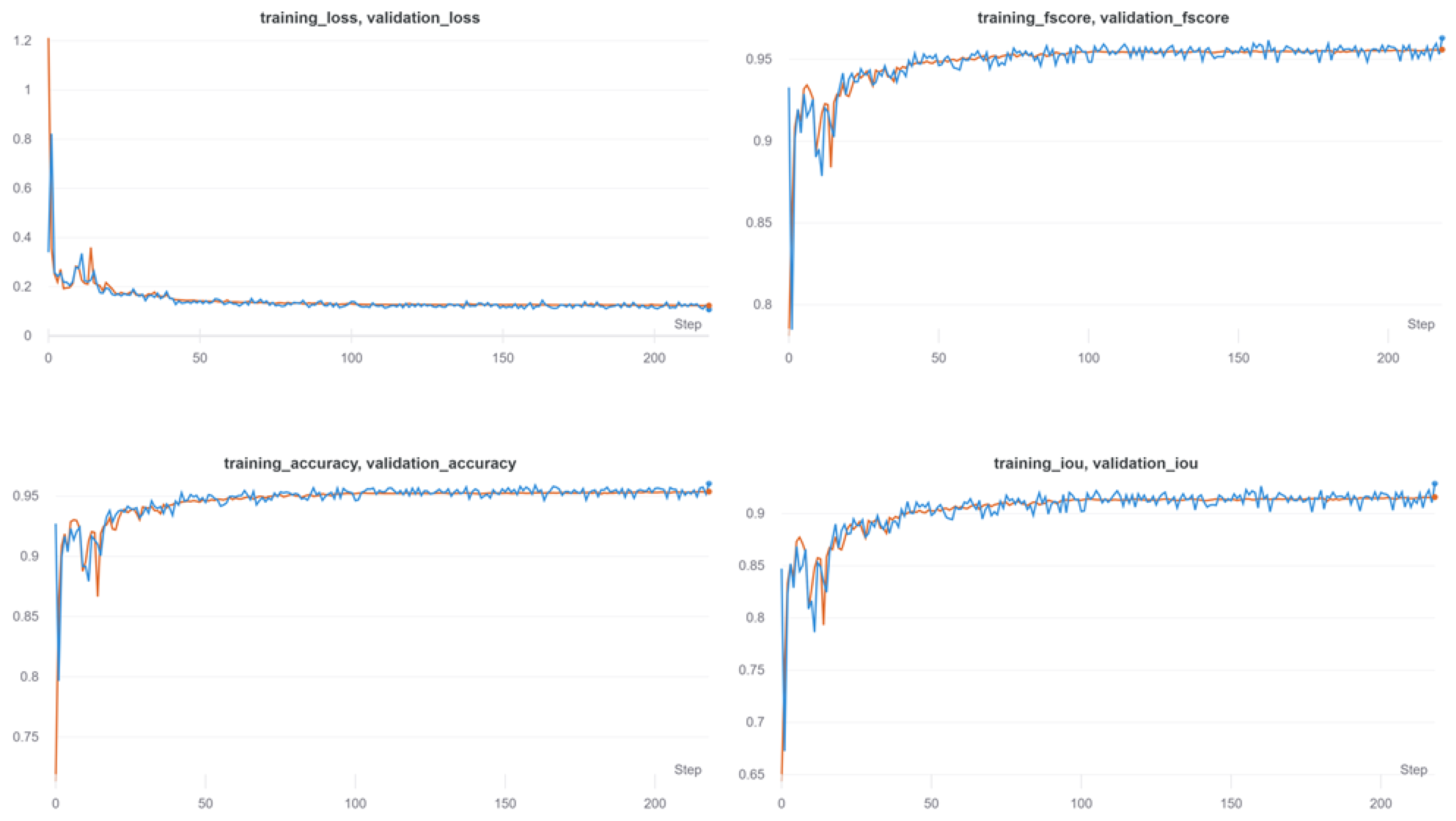
Of all the optimizers, Adam converged to the highest performance metrics, as visible from the percentages reported in
Table 2. The observed training curves are shown in
Figure 5.
As stated earlier, the model encoders were initialized with the pre-trained EfficientNet-B0 weights, so a small learning rate
was used to optimize loss. The learning rate was modulated using different learning rate schedulation strategies, including Cosine Annealing Warm Restart and Multi-step LR. In the end, the simplest one (Multi-step LR) was selected, with learning rate reduced by a factor of
at epochs 2 and 5. The selected
factor is a standard setting in learning schedulation, while the milestones selected to perform the schedulation steps were found by experiments. The model was trained for 10 epochs for a total time of 50 min/run. A batch size of 20 was selected by a trial-and-error procedure in order to saturate the GPU and, therefore, achieve the maximum training speed given the available hardware acceleration. In order to further increase the overall model performance, the net was fine-tuned for 10 more epochs on a small, augmented subset of the original training set starting from the saved weights of the previous run and continuing the optimization process with a very small learning rate. Results are reported in
Table 3.
5. Discussion of Results
In this section, we show the results of the HAFNetE model presented in
Section 3 trained according to the procedure illustrated in
Section 4.3, discuss its features, and highlight the advancements it permits.
5.1. Segmentation Performance Assessment
The first aspect to be evaluated is the overall capability of the model of completing the segmentation task. In particular, it is important to assess whether the newly introduced architecture provides at least the same model performance offered by the original HAFNet. The following results are presented after running the model both in the validation phase and in the test phase. After 1.5 training epochs, the model reached the same performance of the original HAFNet, probably thanks to a combination of:
the pre-trained encoders already providing good basic encoding power, plus
the reduced overall model size speeding up training.
These first training steps set a solid starting point; however, we needed to assert that specific characteristics of the previous model were preserved, as confirmed through several experiments: SegNet-like re-localization capability and re-weighting of decision-level features. As stated in Zhang et al. [
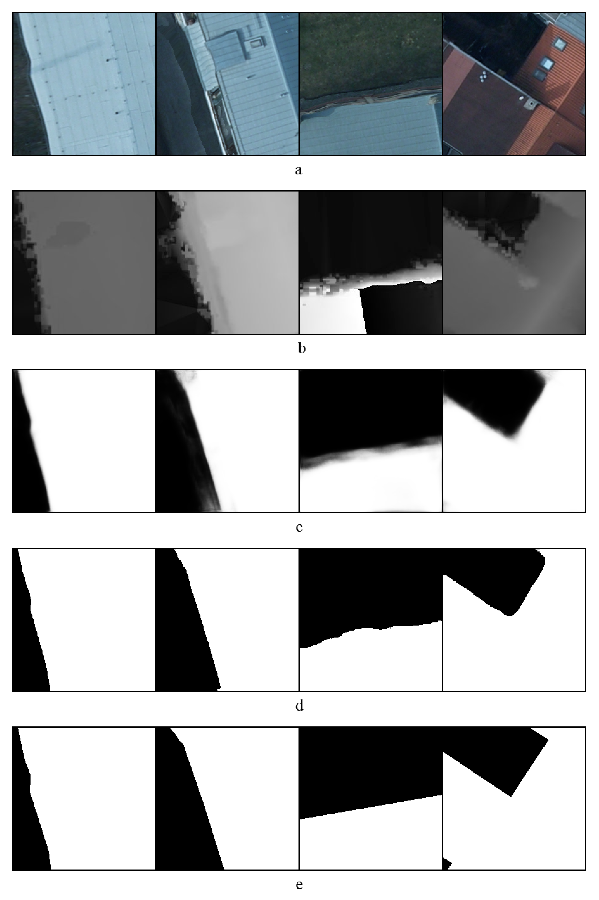
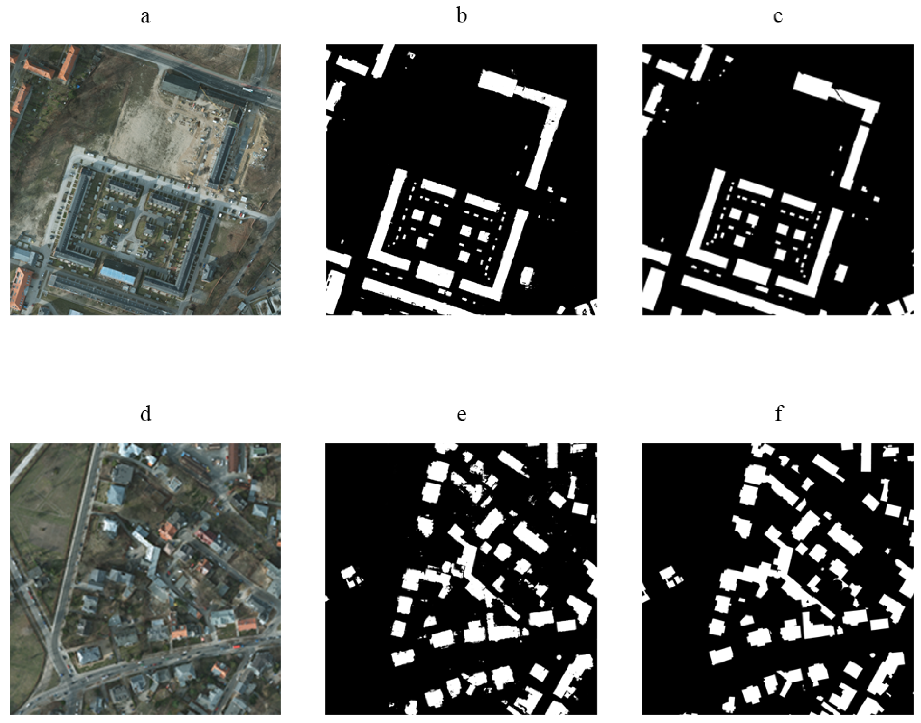
8] regarding adaptability of the scheme to different networks, we can confirm this applies to the HAFNetE model where a U-Net network in each thread replaces the previously proposed SegNet. Moreover, the highly discriminative power granted by the attention fusion block at the decision level remains intact. To give the reader a visual sense of typical results from the proposed method,
Figure 6 shows the final classification results on a set of test patches.
Figure 7 shows, instead, the classification results on a larger scale, providing examples on two entire sample tiles.
Although the biggest advancement from the previous model can be measured in terms of computational efficiency, a segmentation performance improvement can be noticed thanks to the fine-tuning procedure that further enhanced the model’s segmentation capabilities, raising the F1-score to 96.68% and IoU to 93.64%. Refer to
Table 3 for further details. For the reader’s convenience, F1-scores for other state-of-the-art methods on the Potsdam dataset (building) are presented in
Table 4.
Performance metrics show that transfer learning is a suitable technique for achieving great segmentation results also in the Earth Observation domain and that the EfficientNet-B0 encoder is highly capable of extracting discriminative features, even from the very beginning of the training process. In the next paragraph, the benefits of the EfficientNet structure will be presented.
5.2. Novelties Introduced
As discussed in
Section 1 and
Section 3, HAFNet provides a very powerful tool to solve the building extraction problem, yet it involves a huge number of parameters translating into long training and inference times and a bigger memory footprint. The introduction of the Efficientnet-B0 structure in the model architecture conveys two simultaneous benefits, one at the application level and the other at the computational level, as discussed in the following.
5.2.1. Application Level
Features extracted with EfficientNet-B0 encoders are highly discriminative and increase the model segmentation performance from the previously proposed HAFNet. Evaluation metrics show a significant increase in the net capability in detecting and relocating buildings as measured with IoU.
Table 5 shows a performance comparison between the HAFNetE and the HAFNet model.
5.2.2. Resource Level
EfficientNet-B0-based streams architecture led to remarkable achievements not only at the application level but also at a purely computational level. By substituting the VGG16-like encoders in the HAFNet model, the number of parameters shrunk dramatically from 88.978 M to 6.982 M. This size reduction brought multiple benefits that make the HAFNetE model production-ready:
Reduction of training time: the number of weights in a network is directly correlated with the number of gradients updates that the GPU needs to operate to optimize the loss function. A 92% parameters reduction coupled with an extra pre-trained stream translates to a 80% reduction in training time to reach the same model performance.
Reduction of inference time
Reduction of memory footprint: the model weights are encoded as 32-bit floating point variables. To further speed up the inference procedure and limit the overall model size, weights are usually converted to 16-bit floating point. This conversion can sometimes affect the model performance, but, in most cases, the impact is negligible. Under these assumptions, we can estimate the final model size:
vs.
The used memory can be further compressed to a 8-bit fixed point systolic array in order to make the model directly deployable to dedicated AI platforms, such as Intel’s Myriad 2 or Google’s Google Coral 28-nm Tensor Processing Unit (TPU) that features 8 MB of on board memory. The memory footprint of the proposed model is much smaller than that of the reference one. Moreover, its computational and power demand are small; all these factors make it suitable for on-board processing in spaceborne Earth observation platforms.
As we could assess from the recorded metrics, the HAFNetE model can reach state-of-the-art classification performance. However, the most noticeable and relevant advancement from the previously proposed HAFNet model is the efficiency of the overall network. As described in Reference [
9], EO Deep Learning applications are currently relegated to offline processing because models are not properly designed for operating at the edge. In most of the cases, model topology and effective number of parameters are too large to comply with satellites memory and power consumption requirements and that strongly limits the impact that Deep Learning can give to Earth Observation systems. HAFNetE has been engineered taking into account all these requirements and with a deployment-oriented approach. Classical models often disregard memory and computing limitations and, therefore, generally end up not being suitable for deployment as on-board spaceborne systems. HAFNetE represents an example of what DL can provide as an effective tool in real-world EO applications that can work directly on satellites and, consequently, empower new industrial possibilities.
6. Conclusions
In this paper, we considered the problem of mapping buildings in urban areas using an AI-based fusion approach on two different and coordinated data sources, namely high-resolution visible optical data and LiDAR data. In this context, we introduced HAFNetE, a modified version of the previously proposed HAFNet model, which is among the most effective models for the considered tasks, albeit at the expense of computational requirements. The proposed network preserves all the powerful features that characterized the HAFNet model and takes a step forward by achieving better segmentation performance, while drastically reducing the number of parameters. HAFNetE achieved a IoU figure of 93.64% on the popular benchmark dataset of ISPRS 2D Semantic Labeling Challenge [
32]. These features pave the way to new possibilities for real-world exploitation of the devised Attention-aware block scheme. Faster training, shorter inference time, limited computational demand, and limited memory footprint open up possibilities for an on-board AI-powered urban mapping application. The model segmentation performance can probably be pushed to the limit by changing the EfficientNet-B0 encoders with a bigger-sized encoder from the same family, therefore paying a price in terms of training/inference time and memory footprint. Future research plans include incorporation of new state of the art efficient networks in the HAFNetE model, such as, for example, EfficientNetV2 [
41], which has just been released.


