1. Introduction
Human activity on estuaries plays an important role in their dynamics [
1]. Activities such as buildings for urban and industrial occupation, salt-pan creation, fishing, or fish-farming and the action of the natural hydrodynamic agents that control estuarine evolution (river input, tides, and waves) all modify their morphology. An estuary is a system that is very sensitive to modifications of those variables which control its functioning [
2,
3] and, by extension, to all these human activities.
Underwater remote sensing techniques (acoustic and seismic) applied to the geology provide a wealth of information about the morphology of the submarine bed and the structure of submerged floors such as estuarine channels. One of the most commonly used techniques for this is multibeam echosounding [
4], which provides detailed underwater floor information [
5,
6] and allows active bedforms and other surficial structures such as erosional and depositional surfaces to be defined [
7]. Multibeam echo sounding is also able to identify surficial features of deeper deformational structures such as mud volcanoes and pockmarks [
8].
This paper analyzes some of the direct changes made to the estuarine channel by the accumulation of industrial waste in the supratidal margins of the Tinto estuary using underwater remote sensing techniques.
1.1. Location and Regional Ssetting
In the central sector of the Huelva coast is the estuarine system known as the Ria de Huelva. This estuary consists of the shared estuaries of the Tinto and Odiel rivers (
Figure 1). Both estuaries have a common marine sector but function as separate estuaries into the central and fluvial domains [
9]. The Tinto estuary is the eastern branch of this estuarine system and receives contributions from the Tinto river. This river rises in the Huelva mountain range, and its course, which is approximately 100 km long, crosses the province until it flows into the estuary. The drainage basin excises the materials of the Iberian Pyrite Belt, which forms part of the South Portuguese Zone, the southernmost unit of the Variscan Iberian Massif [
10]. The Iberian Pyrite Belt is one of the largest sulfide ore deposits in the world and has been exploited since at least 3000 BC [
11,
12]. From a tectonic point of view, it is astable zone with no vertical movement of tectonic origin, having been described in this area since at least the Holocene period [
13].
1.2. Hydrodynamic Setting
The Tinto estuary is a mesotidal system whose development is conditioned by tides, waves, and siliciclastic contributions it receives from the Tinto river. Fluvial discharge is markedly seasonal, with great interannual irregularity. The average annual contribution is 100.48 hm3, although this mean value is not a significant parameter. The largest floods may exceed 200 hm3, and the contribution of a single month in a rainy year frequently exceeds the annual total of a dry year. In the studied area, maximum flood currents reach values of 1.5 m/s. An example of these floods occurred 1March 2018, reaching flood velocities of 1.2 m/s in the studied area. In contrast, it is common for the river to be almost completely dry when there has been no rain. As a result of acid mine drainage from the Iberian Pyrite Belt, the waters of the Tinto river are strongly acidic, with a mean pH of 2. This type of river water leads to a special pH-mixing that accompanies the typical salt-mixing process.
Waves come mainly from the SW, with mean significant waves of 0.5 m. However, the action of these waves is restricted to the marine domain and does not act on the studied area.
Mean tidal range is 2.10 m, but tides experience major cycles ranging between 3.06 m during mean spring tides and 1.70 m during mean neap tides [
9]. In the studied area, the ebb currents reached by the mean spring tides are 0.95 m/s, whereas the corresponding flood currents are 0.72 m/s. During neap tides, currents are substantially lower, with values for ebb and flood currents of 0.57 m/s of 0.42 m/s, respectively.
Channel depth decreases sharply inland from the confluence of the two estuarine systems from more than 15 m in the shared estuarine channel to a maximum depth of less than 6.5 m in the study area. At the same time, the width of the channel remains constant for over 10 km of its length. For this reason, the tide propagates into the estuary following a hyposynchronic model; hence, the tidal energy is dissipated by friction when entering the estuary. Consequently, for decades, the estuary has maintained a clear depositional character with a mean sedimentation rate of about 3 mm/year [
14].
1.3. Geological Setting
The Holocene estuarine sequence consists of six sedimentary units deposited on a Pleistocene fluvial conglomerate [
9]. These units are (
Figure 2) (1) lower massive muds, (2) lower muddy sands, (3) massive sands, (4) sandy muds, (5) upper muddy sands, and (6) salt marsh muds. The three lower units constitute a transgressive sequence, whereas the three upper units signify a regressive sequence. The total thickness of this sequence can reach up to 30 m in the middle of the estuarine channel and decreases toward the estuarine margins. Units 3 and 4 are characterized by high water content and elevated fluid pressure in pores [
13]. This water cannot migrate vertically because the lower and upper units are fine-grained aquitards.
1.4. Human Influence
A large chemical complex was built along the estuarine margins during the 1960s. The waste from the factories in this complex accumulated on the estuarine banks. One of these residues is phosphogypsum, which is the waste product from the industrial process of manufacturing sulfated fertilizers. From 1964 onward, for decades, phosphogypsum was accumulated in the form of stockpiles. The area covered by the stockpiles is approximately 12 km
2 and is estimated to contain 120 million tons of this waste deposited directly on the estuarine salt marshes [
15]. The tallest of these stockpiles reaches a height of 25 m at some points. This thick artificial deposit exerts an enormous load on the estuarine sediments below. A subsidence process has been observed in the entire waste area. The old marsh surface, which used to be where the intertidal and supratidal zones meet, is now more than 8 m below this level at some points [
16]. This is why the scale of this study is justified.
Considering the subsidence observed in the stockpiles, it was hypothesized that this process might be affecting the areas of the estuarine channel adjacent to the stockpile. Thus, subsidence might extend to the stack margins; on the other hand, an uplift rebound might also occur. Any movement due to subsidence or elevation of the channel floor would result in changes in the dynamics of tidal currents acting on the system. These dynamic changes would be evidenced in several bed features observed in a multibeam analysis. Direct human action on the channel floor was ruled out completely because this channel is not located in a navigable area and has never been dredged or used for dumping.
Following this hypothesis, successive bathymetric surveys were planned to check whether any evolution of these features occurs. In addition, comparison of these successive bathymetries could demonstrate how the vertical processes of uplift and/or subsidence could extend to these under channel estuarine areas. The distribution of elevated and depressed areas was mapped using this method.
2. Materials and Methods
To carry out this study, three campaigns were carried out on 11 September 2017, 17 October 2018, and 19 February 2020. These surveys only covered the northernmost part of the estuarine channel, since the aim was to detect the possible influence of the stacks on their immediate areas.
The survey campaigns were carried out by Nautilus Oceanica SL. An Imagenex Delta T multibeam probe with 240 beams was used, working at a frequency of 260 kHz. Pulse length was set, depending on the maximum slant range, between 5 m/30 µs and 10 m/60 µs. Sampling frequency was 40 Hz. Footprint size was also selected depending on the slant range. Effective beam width was 1.5°. The navigation software used in both campaigns was HYPACK for Hydrographic Surveying connected to anAgGPS332 GPS receiver with differential corrections by OmniSTAR HPto obtain submetric positioning accuracy. The accuracy of gyro/GPS stabilization used the following parameters: roll/pitch 0.03° RMS, heave 5 cm or 5%. And GNSS HDT with a 2 m baseline <0.09°. Parallel navigation tracks were developed parallel to the banks of the estuary to obtain full bottom coverage of the entire study area with an overlap of 20% between lines.
The data obtained in the field surveys were processed and cleaned using HYPACKHYSWEEP software. Since the data were collected during tidal movements, the first step was to carry out a vertical correction to reference the bathymetry points to a datum. The vertical correction was performed using the data for the nearest tide station (Huelva harbor). Over the course of the three surveys, the fluvial discharge was less than 0.1 m3/s. For this reason, any influence of fluvial flood on the water level in the estuary was not considered. The zero was, therefore, established as the extreme equinox low water (EELW) level.
After this correction, all the data obtained were included in triple coordinate tables (x, y, z). Each of the tables corresponding to the different bathymetries included more than 2.7 million points. From these data, digital topographic processing was carried out using the program Surfer 13. This software allows interpolation meshes (grids) to be created which can then be represented two- or three-dimensionally. The grids were obtained using triangulation as an interpolation method and with a grid spacing of 0.25 m.
The comparison between different bathymetries was carried out by means of the algebraic subtraction of grids (the Grid Math function in Surfer 13). This comparison was made under the assumption that the later bathymetry would be above the previous one. Thus, positive volumes indicate areas that elevated, while negative volumes indicate areas that depressed. In this regard, it must be considered that ascents may be due to tectonic uplift or depositional causes, while decreases may be due to subsidence or erosion.
3. Results
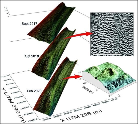
The multibeam echosounder provides numerical bathymetric elevation results that can be used to produce a digital elevation model (DEM) to be represented in the form of isobath maps, shaded relief, or a 3D surface. In this case, isobath maps do not offer a visually intuitive representation, since the relief geoforms are on such a small scale that they result in isobath lines so intricate that they make interpretation difficult. On the other hand, 3D diagram blocks do allow an almost real visualization of the bed structures (
Figure 3) and have been used for the description and interpretation of morphological features.
However, these blocks cannot be reproduced at the proper scale in a scientific paper as they cover a very wide area. For this reason, this paper only uses this type of representation to show morphological details of small areas. Lastly, the shaded relief allows for good visualization of floor features, with an appearance reminiscent of side-scan sonar records. This type of representation was chosen to show the features over the total surface of the studied area.
The paragraphs below provide a description of the features observed in each of the bathymetries. In addition, the data obtained from comparing the data for the three bathymetric surfaces are analyzed.
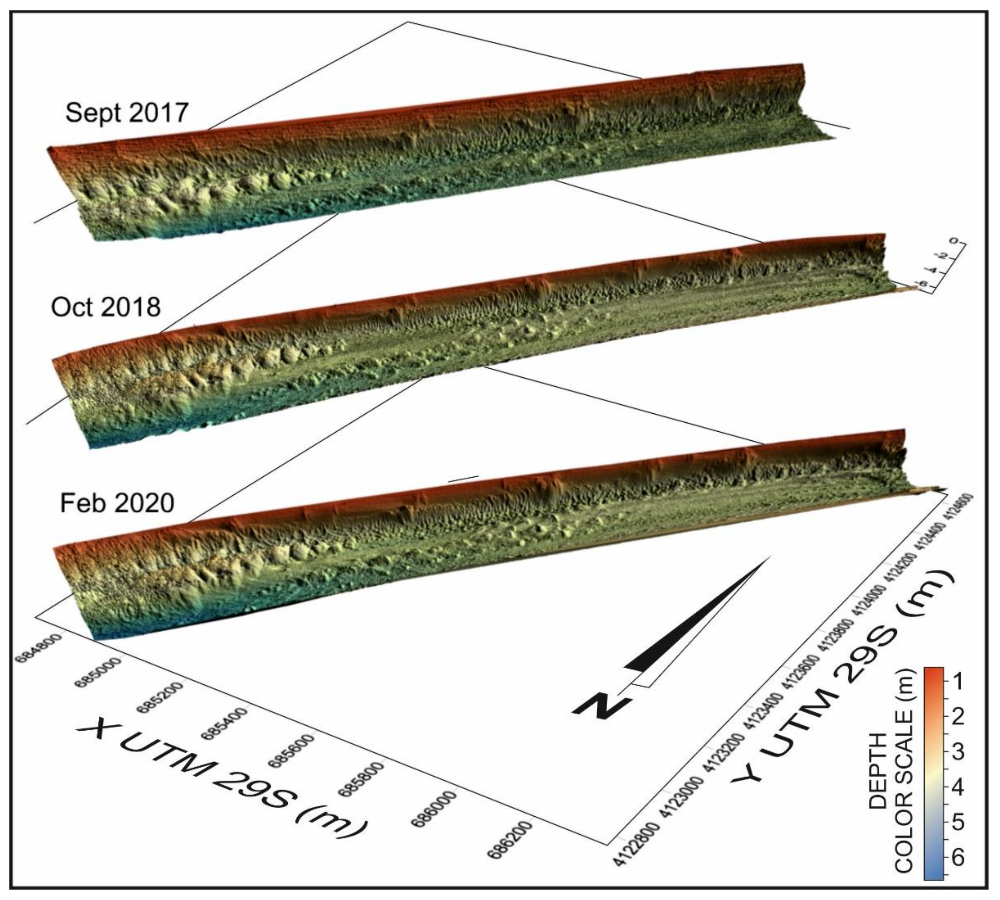
3.1. Bathymetry from September 2017
During the bathymetric survey, a windstorm with waves more than 1 m high reached the coast. The presence of big waves into the estuarine channel made it difficult to capture data and caused poor vertical adjustment of the different record lines. All this resulted in low-quality visualization of the floor details, but allowed, nevertheless, the analysis of large features and relief distribution (
Figure 4).
The shallower areas correspond to the northeastern edge of the study area, where the emerged margin occupied by the stockpiles is located. The steepest slope corresponds to an escarpment that separates the estuarine channel from the supratidal areas reclaimed by the wastes. In the southwest sector stands out the presence of several anastomosing bulges with dozens of meters in diameter. This bulge field is separated from the escarpment by a runnel. It is also observed a crestline consisting of decametric elevations developed in a subparallel way to the estuarine margin. The conic shape of these metric elevations suggests that they could correspond to mud volcanoes. Some observed features of the channel bed could be interpreted as bedform fields. These structures are developed in a band parallel to the escarpment. In the northeast area, a wide surface developed structures that could be interpreted as evidence of erosion.
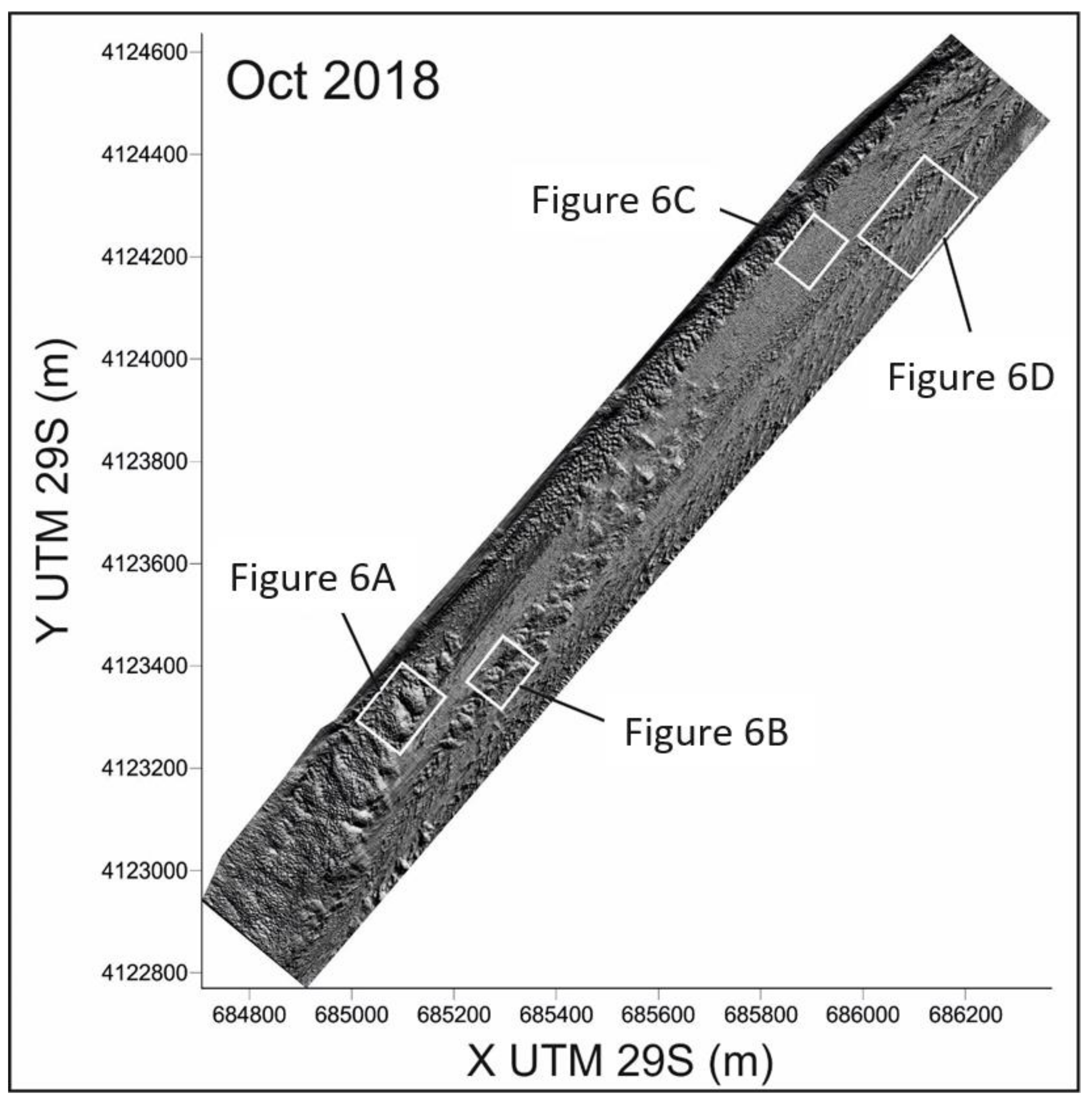
3.2. Bathymetry of October 2018
The bathymetry performed in 2018 not only had a better fit of data between the lines obtaining a better resolution, but also covered a wider area than that performed in 2017. This bathymetry allowed a better visualization of the floor features (
Figure 5). The good resolution of this new bathymetry allows us to observe how the bulge field on the southwest margin described in the previous bathymetry changes geometry and dimensions. The surface of these bulges reveals an irregular, rough appearance (
Figure 6A), which suggests the presence of erosional processes. It is significant that the runnel separating this bulge field from the escarpment, observed in 2017, has nearly completely disappeared in this new bathymetry. The ridge formed by the conical elevations observed in 2017 was much more evident in 2018. This southernmost part of the crest is formed by attached individual cones separated by depressions (
Figure 6B), whereas the northern part is formed by individual cones. Between this ridge and the escarpment, fields of bedforms (3D dunes) have developed. Other dune fields also extend into the northeast area, bordering the escarpment (
Figure 6C). These indicate a sedimentary bypassing of sandy materials from the fluvial area to the estuarine mouth. On the other hand, the erosive features of the deeper area are also evident (
Figure 6D). It is important to note that the areas of lower slope displaying erosive features have moved toward the southeast margin if compared with the previous bathymetry.
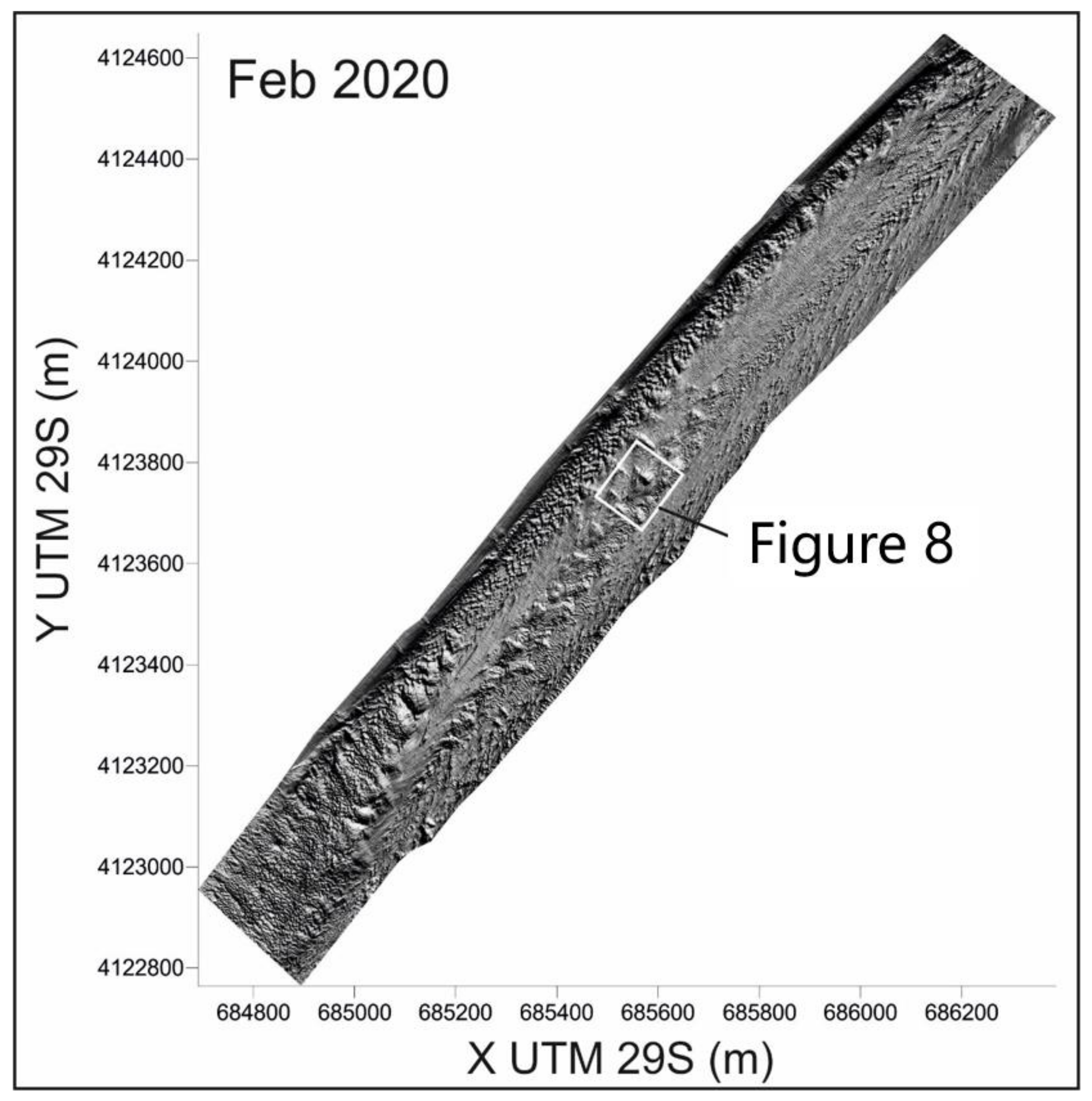
3.3. Bathymetry from February 2020
At first sight, it would appear that there are not many differences between this bathymetry (
Figure 7) and that surveyed in October 2018. However, some subtle details can be observed. On the one hand, the surface of the bulge field changed slightly, displaying an even rougher surface now. On the other hand, the relief of the conic features seems to be more pronounced. To the north, some individual cones reach 50 m in diameter and rise more than 5 m from the bed average; thus, they can now be well observed (
Figure 8). Some new cones are more evident just in the high-sloped channel margin in the northeast area. The bedform fields are now less developed, whereas the erosive surfaces are wider in this bathymetry and extend into areas occupied by bedforms in the previous survey.
3.4. Quantitative Comparisons of Bathymetries
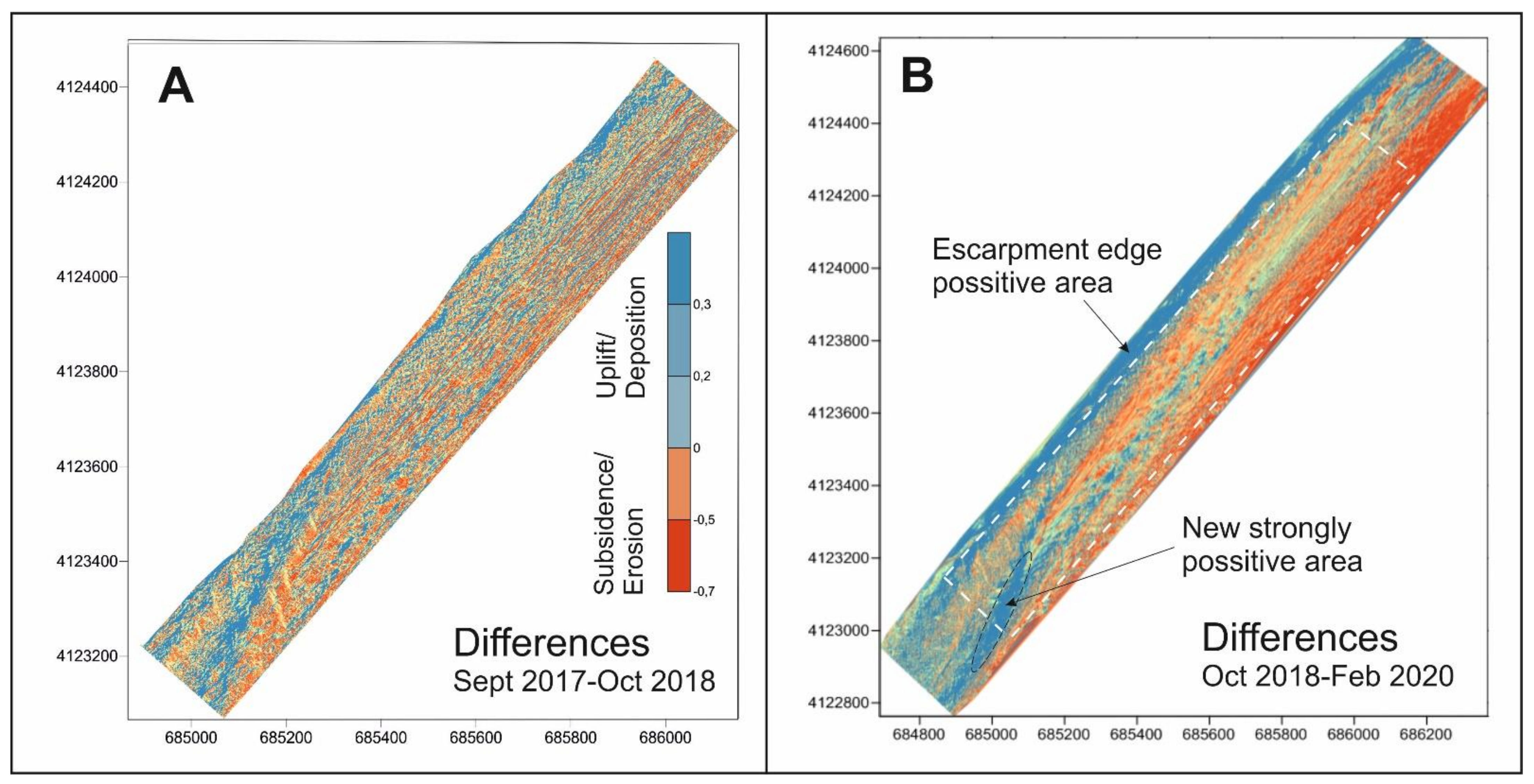
The bathymetries were compared quantitatively using algebraic subtraction of numerical grids for two successive datasets. These new grids obtained from the quantitative comparison were represented in two maps of differences (
Figure 9). In these maps, the areas where the later surface is higher than the previous one are represented in blue tones, whereas the areas where the later surface is lower than the previous one are represented in red tones.
It must be borne in mind that a later surface can be located above a previous one as a result of uplift or sedimentation processes. By contrast, a later surface can be located under the previous one due to subsidence or erosional processes. A combination of both tectonic and sedimentary processes can result in positive, erosive, or neutral balances.
3.4.1. Differences between September 2017 and October 2018
The comparison of these two bathymetries (
Figure 9A) covers only the area of the bathymetry from September 2017, which is smaller than the other two. The result of this comparison is not high-resolution, due to the low accuracy of the bathymetry from 2017. Nevertheless, some general observations can be made. The negative surface area is wider than the positive surface area. The quantified size of both positive and negative surface areas appears in the upper rows of
Table 1. According to these data, 54.45% of the studied area corresponds to negative areas. The positive and negative volumes were also compared (the lower half of
Table 1). The negative volume is 25,943.53 m
3 larger than the positive volume. The map shows an irregular distribution of negative and positive areas. The positive areas are concentrated in a fringe located at the base of the eastern escarpment and in the bulge field area (southwest). However, the rough top of the dome area presents some net negative surfaces.
3.4.2. Differences between October 2018 and February 2020
A comparison of the surfaces in October 2018 and February 2020 (
Figure 9B) offers better results, since these are both high-resolution bathymetries. In addition, the area covered is larger. As in the previous comparison, positive areas developed along the escarpment, as well as into the bulge field; however, in this case, it is very visible that the ridge of cones is clearly positive. The southeastern fringe of the study area (the central part of the estuarine channel) is strongly negative, and the runnel located between the ridge and the escarpment is also negative. Note that this area was covered by bedforms in 2018 but presents mostly erosive features in 2020.
The quantifications of positive and negative surface areas and volumes offer the most balanced results in this case (
Table 2). The negative volume continues to be greater than the positive one, but only by 3644.86 m
3. At this point, it must be borne in mind that the second analysis includes a strongly positive new area located in the southwest, to which the bulge field extends.
4. Interpretation and Discussion
An analysis of the observed surficial structures allows us to distinguish two well-differentiated types: structures of hydrodynamic origin and structures of unidentified origin. In turn, two types of structures of unidentified origin differ: cones and bulges. The conical structures have a scale of tens of meters. Bulges are larger-scale structures, which can reach up to 100 m in diameter and more than 4 m in height difference between their edges and their center. A direct human origin of these structures is rejected, because the estuarine channel is not navigable in this area and has never been dredged in the last 50 years.
The clear volcanic shape of some of the cones observed in 2018 and 2020 suggests that these could be mud volcanoes. These structures have classically been interpreted as a result of the extrusion of liquefied material from deeper sedimentary units. Mud volcanoes are described as conical geological features attributed to the eruption of ascending fluids (gas or water) or fluidized sediments from deep sedimentary layers [
17]. The biggest and most highly dynamic mud volcanoes develop through gas escaping in compressional settings [
18], but smaller edifices can also develop due to overpressured fluids and sediments at depth [
19]. The presence of extruding structures on the margin of the stockpiles could indicate that some of the estuarine units (units 3 and 4, composed of sand and sandy mud between muddy aquitards) were fluidized, migrating laterally and injecting vertically along the margins, where the pressure is lower (
Figure 10). In this case, the volcanoes would be formed by muddy sands instead of muds. Thus, they must be more properly called sand volcanoes or simply sediment volcanoes.
As for the hypothesis of an extrusive origin, the bulge field could be interpreted as the result of anastomosing small domes. Domes can have different origins (magmatic, tectonic, and sedimentary). A type of dome can be produced by a mixture of tectonics and sedimentary processes related to diapirism [
20]. Diapirs are structures formed by ductile material extruding massively to the surface as a result of high-pressure deformational processes at depth. A large number of diapirs are formed by salt [
21], but shales can also extrude in the form of diapirs, piercing and warping the upper sediments and forming domes [
22]. The scale of diapir-induced domes varies, depending on the nature of the extruded material and the pressure that causes the extrusion. On some occasions, it is possible that the extruding material does not fully reach the surface, but it can bend the upper units, shallowing its upper part. In this case, it can lead to hydrodynamic disequilibrium, and the shallower areas of the bulge can be eroded and partially or totally dismantled. The process described may be a good explanation for the presence of a rough texture on the bulge field surface and the negative character in
Figure 9.
In some settings, diapir-induced domes and sediment volcanoes can appear together, linked to the same overpressure processes [
23]. In the study area, the possible interpretation of these structures as sediment volcanoes and domes could be attributed to overpressure caused by the stockpiles. The stockpiling of phosphogypsum on the marsh to a height of 25 m means that the sediments from the lower estuarine unit have doubled in load in just 46 years (1964–2010). This is the cause of the subsidence of more than 8 m at some points (
Figure 10), as deduced from the height of the contact between the salt marsh facies and the gypsum deposits observed in drilling cores [
16]. This subsidence necessarily leads to deformation of the sedimentary units deposited under the stack. It is also possible that the old marsh surface was not exactly horizontal before the gypsum piling was begun. In any case, that implies the possibility of errors of dozens of centimeters in the calculation of the subsidence values. Nevertheless, even despite these possible errors, values of subsidence of several meters are undeniable.
Conic shapes (which may or may not be sediment volcanoes) are more frequent in a linear chain along the central axis of the studied area and diminish to the northeast sector, while bulges are concentrated in the southwestern portion, coinciding with the southeastern edge of the stockpiles. This could indicate rising overpressure from NE to SW.
Comparison of the bathymetries from September 2017, October 2018, and February 2020 indicates rapid evolution reflected in bathymetric changes. In all cases, the highest rates of ascent of the bed are distributed on the right margins of the stockpile, while the channel deepens toward the central axis of the estuary (
Figure 9).However, it must be borne in mind that the vertical movements of the bed may be related to tectonic uplift or subsidence, as well as to the sedimentary processes of deposition and erosion. In this regard, it might be interesting to analyze the magnitude of the recorded vertical changes. The maximum observed positive vertical changes are on a centimeter scale, whereas the maximum depositional rates described in this area in previous papers are of millimeter magnitude [
13]. In addition to the previous data, the presence of bedform fields in some of the positive areas could suggest centimetric vertical changes of depositional origin when the fluvial system introduces significant amounts of sands. Out of the ripple fields, the presence of positive changes could be attributed to uplift processes. In addition, the presence of depositional structures (bedforms) and erosive surfaces may provide some keys to interpretation of the processes.
The low resolution of the 2017 bathymetry prevents very good results being obtained from the comparison between September 2017 and October 2018 (
Figure 9A). Nevertheless, some general observations can be made. The development of a large field of megaripples is observed along the bank of the stack in 2018, which indicates that it is a depositional area. However, the surface in 2018 is below that in 2017, and this area corresponds to a negative surface. Note that an important flood occurred during storm Emma (1 March 2018), before the second bathymetric survey. During this storm, the flood reached current velocities of 1.2 m/s, maintaining these conditions for 16 h. This second surface can be the result of a first erosion caused by the flood that occurred during storm Emma and a further deposition of sandy bedforms. A scenario where subsidence processes are responsible for the net bathymetric descent despite it being a depositional field could also be possible. At the same time, the deeper area located along the eastern margin of the study area is also depressed but displays clear erosive features. In this case, the bathymetric descent could be attributed to just erosional processes.
The comparison between October 2018 and February 2020 (
Figure 9B) offers better results since both bathymetries are high-resolution and have wider coverage. In this case, a bathymetric shallowing is observed along two longitudinal bands: one along the border between the channel margin and the stockpiles (NW long border of the study area) and the other along the central area, coinciding with the chain of mud volcanoes. Both positive alignments converge in the SW, right at the bulge field. Some of these areas were covered in dunes in 2018 but in erosive features in 2020. In this case, under erosional conditions, the shallowing implies an uplift origin. The shallowing of the chain of cone-shaped features could be explained by an increase in the volume of each individual cone.
The negative surfaces are concentrated along the SE portion of the studied area approaching the central part of the estuarine channel. This area coincides again with the distribution of erosive features on the bed. Consequently, it can be deduced that the deepening is due to erosional processes. It has already been commented that the bulge field presents a general uplift, but its upper surface presents some erosive areas (as well as erosive features). It is possible that this large structure might be eroded on its upper surface during a general uplift process.
From these observations, it follows that the possible action of processes involving vertical displacement of the ground caused by the overpressure exerted by the stacks acts in conjunction with the hydrodynamic processes of sedimentation and erosion caused by tidal currents. In this context, the question arises as to whether there is any influence on each other in view of the dynamic regime of the estuary. A possible answer might be found in channel section changes caused by vertical movements of the estuarine bed. From a hydrodynamic point of view, the channel must adapt to an equilibrium profile in line with the velocities of the tidal currents. These velocities depend directly on the tidal prism and the flow section [
24]. If there are no changes in the tidal prism, the currents should remain stable, as it controls the volume of water passing through the flow section. However, any vertical movement in the bed will produce changes in the flow section, which will lead to changes in the velocities of flood and ebb currents. The erosional processes can occur during strong currents occurred during spring tides, as well as increase during fluvial floods. Subsequently, any rise of the ground, such as that observed in the study area, will result in a decrease in the flow section and, consequently, an increase in the velocities of the tidal and fluvial flood currents. Higher flow speeds will lead to an increase in sediment transport capacity. This explains the appearance of both bedform fields and erosive zones. Generally speaking, higher current velocities will tend to erode by increasing the flow section until a new equilibrium profile is reached. In short, movements of the beds caused by stacking phosphogypsum bring with them dramatic changes in the hydrodynamic regime of the estuary.
The possibility of the influence of large fluvial floods during the second studied period was rejected for four reasons. On the one hand, the Tinto river is normally a low-regime river which is pluvial in nature. No floods occurred between the two last surveys. On the other hand, the surveys were carried out after months of low river flow and under the tidal domain. Lastly, in this system, the fluvial water volume during a flood is only about 10% of the maximum tidal prism [
9].
Although there is abundant literature on the influence of this type of stockpile on the environment where they are located, most of the papers focused on the geochemical influence of them in the form of environmental pollution (e.g., [
25,
26]), and there are no studies that document changes similar to those described in this work.
However, the results of this work should be supplemented by evidence documenting the existence of diapirs under bulges and fluid escape chimneys under cones in order to verify the hypothesis that these are really domes and sediment volcanoes. Consequently, a seismic profiling survey has been planned, the results of which are being analyzed and will be the subject of further work.
Independently of the origin of these bathymetrical changes, it is clear that the stockpile introduces significant changes in the behavior of the channel floor. A possible medium-term vision of this process seems to indicate that the continuous subsidence could cause a instability in the slopes of the stockpile. The collapsing of industrial waste and its causes have been analyzed by the US Environmental Protection Agency [
27], albeit from a generalist point of view, without delving into the specific processes. Ground subsidence and liquefaction are cited as possible processes acting under the stacks. Both of these can constitute a real hazard for sudden collapse during an earthquake.


