Mapping a Paddy Rice Area in a Cloudy and Rainy Region Using Spatiotemporal Data Fusion and a Phenology-Based Algorithm

Abstract

The timely and accurate mapping of paddy rice is important to ensure food security and to protect the environment for sustainable development. Existing paddy rice mapping methods are often remote sensing technologies based on optical images. However, the availability of high-quality remotely sensed paddy rice growing area data is limited due to frequent cloud cover and rain over the southwest China. In order to overcome these limitations, we propose a paddy rice field mapping method by combining a spatiotemporal fusion algorithm and a phenology-based algorithm. First, a modified neighborhood similar pixel interpolator (MNSPI) time series approach was used to remove clouds on Sentinel-2 and Landsat 8 OLI images in 2020. A flexible spatiotemporal data fusion (FSDAF) model was used to fuse Sentinel-2 data and MODIS data to obtain multi-temporal Sentinel-2 images. Then, the fused remote sensing data were used to construct fusion time series data to produce time series vegetation indices (NDVI\LSWI) having a high spatiotemporal resolution (10 m and ≤16 days). On this basis, the unique physical characteristics of paddy rice during the transplanting period and other auxiliary data were combined to map paddy rice in Yongchuan District, Chongqing, China. Our results were validated by field survey data and showed a high accuracy of the proposed method indicated by an overall accuracy of 93% and the Kappa coefficient of 0.85. The paddy rice planting area map was also consistent with the official data of the third national land survey; at the town level, the correlation between official survey data and paddy rice area was 92.5%. The results show that this method can effectively map paddy rice fields in a cloudy and rainy area.

1. Introduction

Paddy rice, as a staple food, feeds almost half the world’s population [1]. It is of important to obtain the spatial distribution of paddy rice in a timely and accurate fashion [2,3,4,5,6]. Mapping paddy rice is significant for understanding and evaluating regional, national, and global issues such as food security, climate change, disease transmission, and water resource utilization [6].

Southwest China is a key paddy rice planting area. Affected by the climate, this area has a lot of precipitation and is cloudy and foggy. With the continuous development of satellite remote sensing technology, our ability to monitor and map paddy rice fields has improved. Time series of remote sensing data, such as MODIS and Landsat, have been widely used in paddy rice monitoring [7,8]. Higher spatial resolution data can improve the mapping accuracy of paddy rice [9].

With the development of time series images, phenology-based algorithms have been developed [8,9,10,11]. Paddy rice fields are a mixture of water and rice plants, which have unique physical characteristics during the flooding and transplanting stages. We can use the relationship between the land surface water index (LSWI) and the normalized difference vegetation index (NDVI) or enhanced vegetation index (EVI) to identify the features. At present, transplanting-based algorithms have been widely used for mapping paddy rice fields in many areas [10,11]. For example, Xiao et al. used a transplant algorithm to map paddy rice, and used MODIS data to generate paddy rice distribution maps in South China, South Asia, and Southeast Asia [8,11]. Zhang et al. used time series vegetation index data to obtain a map of paddy rice distribution in Northeast China in 2010 [12]. Dong et al. obtained the dynamic changes of paddy rice planting area in Northeast China from 1986 to 2010 through time series Landsat images and phenology-based algorithms [13].

However, optical satellite remote sensing data are affected by cloud and rain images, and there are few effective images in southwest China. In the course of this research, we searched for valid images (cloud coverage < 60%) in Southwest China in 2020. The results show that Landsat 8 OLI (temporal resolution, 16 days) has about 12 images, and Sentinel-2 (temporal resolution, 5 days) has about 20 images. There is a lack of sufficient time series data and appropriate methods for relevant research in Southwest China [14]. In order to improve the availability of the image, it is necessary to remove clouds from images. However, cloud coverage in cloudy and rainy areas is frequent and lasts for a long time, and a single data source after cloud removal is still unable to establish time series data satisfying paddy rice monitoring. Therefore, the development of a method that combines the cloud removal method with the spatiotemporal fusion model may provide an effective method for paddy rice mapping in cloudy and rainy areas. Removing thick clouds from the image is a necessary condition to improve its quality and usability [15]. Generally speaking, the method of removing thick clouds requires cloudless images as auxiliary images to restore the spectral information occluded by clouds [16,17,18,19]. Melgani proposed a contextual multiple linear prediction (CMLP) method to reconstruct spectral values of cloud areas in Landsat images [18]. Zhu et al. developed a modified neighborhood similar pixel interpolator (MNSPI) method to remove thick cloud pollution from satellite images over land [15]. This method can maintain the spatial continuity of the filled images even when the time interval between the auxiliary image date and the predicted image date is long [20]. As compared with CMLP, this method has a better effect of restoring image information [15]. When cloudy and auxiliary images are acquired in different seasons, the reflectance value estimated by the MNSPI method is more accurate than the CMLP result.

Fusion of high-spatial/low-temporal resolution data with high-temporal/low-spatial resolution data (such as Sentinel-2 and MODIS) can generate high-temporal/high-spatial resolution data. In previous studies, many spatiotemporal fusion models have been proposed and applied, such as the spatial and temporal adaptive reflectance fusion model (STARFM), the enhanced STARFM, and the robust adaptive spatial temporal fusion model (RASTFM) [21,22,23]; however, these fusion algorithms have certain limitations [24]. First, the complexity of land cover changes in homogeneous or heterogeneous landscapes is not fully considered. Secondly, most spatiotemporal fusion algorithms require two or more low–high-spatial resolution images as prior information. Aiming at the limitations of the aforementioned spatiotemporal fusion methods, Zhu et al. proposed a flexible spatiotemporal data fusion (FSDAF) model [24]. Its goal is to more accurately predict high-resolution images of non-uniform areas by capturing gradual and sudden land cover type changes.

At present, the spatiotemporal fusion model has proved its ability in crop type detection [25,26,27,28]. For example, Zhu et al. used the STARFM model to fuse Landsat and MODIS images, combined with support vector machines (SVM) to classify crop types in 2017 [25]. A recent study used fusion images of several key dates and used a supervised random tree (RT) classifier to map paddy rice fields in Hunan, China [26]. Cai et al. used the RASTFM model to fuse MODIS and Sentinel-2 data, combined with the random forest (RF) method to map paddy rice [27]. Yin et al. used the STARFM model to fuse Landsat and MODIS data. On this basis, they used a phenology-based algorithm to map paddy rice fields [28].

In this study, we aimed to use the cloud removal interpolation method and data fusion method to reconstruct remote sensing time series data and map paddy rice areas combining these with a phenology-based algorithm, and provide a new method to map paddy rice in cloudy and rainy areas. The specific steps were as follows: (1) the MNSPI approach was used to remove clouds and interpolation for Sentinel-2 and Landsat 8 OLI images with 30–60% cloud coverage; the quality assessment (QA) band of MODIS product was used to remove clouds from MODIS images; (2) the FSDAF model was used to fuse Sentinel-2 images and MODIS images to obtain Sentinel-2-like fusion images; (3) a dataset with a high spatiotemporal resolution of the study area was constructed based on the three kinds of remote sensing data, and we mapped paddy rice combined with a phenology-based algorithm; (4) we used field survey data and official statistics to evaluate the accuracy of the final paddy rice map.

2. Study Area and Data

2.1. Study Area

Yongchuan District is located in the west of Chongqing, China, at 105°38′–106°05′E longitude and 28°56′–29°34′N latitude, covering an area of 1576 square kilometers (Figure 1). It belongs to a subtropical monsoon humid climate, with an average temperature of 18.2 °C, a maximum temperature of 39 °C, a minimum temperature 2 °C, and an average annual rainfall of 1042.2 mm. In Yongchuan District, there are mainly low mountain troughs, hills, terraces, and other landform types. Under relatively favorable climatic conditions, Yongchuan District is a suitable area for planting paddy rice, and it is a typical mountainous and hilly paddy rice planting area. Checking the historical weather data from the China Meteorological Network, the weather of Yongchuan District in 2020 was 41% overcast, 35% cloudy, 9% rainy, and 15% sunny (Figure 2). It belongs to a cloudy and rainy area. Three-quarters of the days are covered by clouds, and there are fewer high-quality optical remote sensing images. Therefore, selecting this area for paddy rice mapping research has certain reference significance for paddy rice mapping in cloudy and rainy areas.

2.2. Data and Preprocessing

2.2.1. Optical Remote Sensing Data and Preprocessing

The Sentinel-2 satellite is a high-resolution multispectral imaging satellite consisting of two satellites, 2A and 2B. The multispectral instrument (MSI) that it carries has 13 bands with different spatial resolutions (10, 20, and 60 m). The revisit period of one satellite is 10 days, and the revisit period of two satellites is 5 days. We selected the B2 (blue), B3 (green), B4 (red), B8 (NIR), and B11 (SWIR) bands of valid images (<60% cloud cover) from January to November 2020 as the study target. The download address is the United States Geological Survey (USGS) website. The downloaded data were only Level-1C data, and no atmospheric correction was performed. We used the Sen2cor processor for atmospheric correction (http://step.esa.int/main/third-party-plugins-2/sen2cor/, accessed on 18 March 2021). In addition, because the spatial resolution of the microwave band (B11) is 20 m, and the remaining bands are 10 m, we resampled the B11 band through the Sentinel Application Platform (SNAP) to give a spatial resolution of 10 m.

Landsat 8 (OLI) data use its secondary product, surface reflectance data, after atmospheric correction. The temporal resolution is 16 days, and the multi-spectral band spatial resolution is 30 m. The download address is the USGS website. We selected valid images from January to November 2020 with a coverage of cloud < 60%.

MOD09GA is a daily surface reflectance product with a spatial resolution of 500 m. We used the official website of the National Aeronautics and Space Administration (NASA) to download images of the study area in 2020. After the download was complete, the data were preprocessed. We used MRT (MODIS Reprojection Tool) for data format conversion and map projection conversion. Then, we used the quality control layer to remove invalid values in the image.

The map projection of all the data was a UTM (WGS84) projection, Zone 48 (North). The band used was also the same. We used ENVI software for layer stacking and image cropping.

2.2.2. Paddy Rice Crop Calendar

Paddy rice planting in Chongqing is dominated by single-season rice. We checked the Chongqing Agricultural Technology Station (http://www.cqates.com/, accessed on 9 October 2020) and obtained the paddy rice planting calendar in Chongqing (

Table 1. Paddy rice planting calendar in Chongqing, the study area belongs to the western part of Chongqing.

Month	Jan.			Feb.			Mar.			Apr.			May.			Jun.			Jul.			Aug.			Sep.			Oct.			Nov.
Ten-Day	F	M	L	F	M	L	F	M	L	F	M	L	F	M	L	F	M	L	F	M	L	F	M	L	F	M	L	F	M	L	F	M	L
West							1	1	1	2	2	2	3	3	3	4	4	4	4	5	5	5	6
Northeast							1	1	1	2	2	2	3	3	3	3	4	4	4	4	5	5	5	6
Southeast									1	1	1	1	2	2	3	3	3	3	4	4	4	4	5	5	5	6

Note: 1, sowing; 2, flooding/transplanting; 3, tillering to stem elongation; 4, panicle initiation to heading; 5, filled/milky; 6, maturity and harvest.

). The paddy rice growing seasons are slightly different in western Chongqing, northeastern Chongqing, and southeastern Chongqing. Different altitudes, rainfall, and temperature affect the growing season of paddy rice.

Yongchuan District belongs to the Western Chongqing area. Farmers usually raise seedlings in March, and it takes about one month to enter the transplanting period. The flood signal is an important feature that distinguishes paddy rice from other crops. Paddy rice is transplanted in early April, and the tillering period begins in mid-to-early May. The paddy rice grows rapidly in June and July, covering the entire field, and is harvested in mid-August.

2.2.3. Field Survey Data

In order to assess the accuracy of the results, we conducted a field survey in the study area from 31 May to 1 June 2021. The selection of sampling sites included paddy rice sites and non-paddy rice sites (forests, built areas, water bodies, and crops). We used a Real-Time Kinematic (RTK) measuring instrument to obtain the GPS coordinates of the sample point and took field photos of the sample point. Finally, there were 511 field survey sites, 297 paddy rice sites, and 214 non-paddy rice sites (Figure 3). It is worth noting that this study focuses on mapping paddy rice in the study area in 2020. We ensured that each sample site selected in the field survey in 2021 was consistent with the 2020 land cover type through field inquiries and the use of Google Earth historical imagery.

2.2.4. Auxiliary Data

The auxiliary information was mainly the land-use data of the study area in 2020 and the official statistical data used to verify the accuracy of the results. We used existing land-use data to establish mask information for other land types (built area, water body, forest, and grassland) and effectively improve the accuracy of the result. The land-use data used in this study were the 10 m land cover data product released by Esri in 2020 (https://livingatlas.arcgis.com/landcover/, accessed on 10 July 2021). This land cover data product includes 10 types of land such as forest, grassland, built areas, and shrubland. The overall accuracy of the product is 0.85 [29]. Official statistics include two categories. The first category is the sown area of paddy rice in Yongchuan District in the 2021 Statistical Yearbook released by the Statistics Bureau of Yongchuan District, Chongqing. The second category is the third national land survey data. First, we loaded the national land survey data into ArcMap software to extract paddy field data. Then, we overlaid vector files of the town boundary and counted the area of paddy fields in each town. The two types of data were used at different levels (district and town levels) to verify the accuracy of the results.

3. Method

The spatiotemporal data fusion and phenology-based paddy rice mapping methodology mainly involved the following steps (Figure 4): (1) removing thick clouds, i.e., for the Sentinel-2 and Landsat 8 OLI images, thick clouds were removed with MNSPI approach and, for the MODIS images, clouds were removed with the QA band; (2) FSDAF prediction using images after preprocessing (Sentinel-2, MOD09GA); (3) mapping paddy rice using the phenology-based algorithm; and (4) accuracy assessment.

3.1. Removal of Thick Clouds

MNSPI is an approach proposed by Zhu et al. [15] to remove thick clouds based on a neighborhood similar pixel interpolator. Initially, this method was developed to address the strip loss problem of Landsat ETM+ [20], according to the idea of the original NSPI, using the information of neighboring similar pixels to restore the spectral values of cloudy pixels. However, clouds are usually large clusters. In order to explain this difference in spatial pattern, the NSPI method needs to be modified.

The modified steps were as follows: First, two images are required, an auxiliary image acquired on date $t_1$, and the auxiliary image should be cloudless for the clouded part of the clouded image acquired on date $t_2$. Second, extract the cloud mask from the cloud image. The cloud mask can be extracted with the help of the QA band of the image, or the cloud mask layer can be established by visual interpretation. Third, a large window covering the cloud layer is established to find the closest pixels around the cloud layer that meet the spectral similarity criteria as similar pixels. Fourth, spatial distance ($D_i$) and spectral distance ($RMS{D}_i$) are both normalized. Finally, determine the weights and predict the results. The weight can be determined by the relative spatial distances from the target pixel to its similar pixels and to the cloud center. The coordinates of all cloud pixels are averaged to calculate the cloud center. Finally, the value of the target pixel can be predicted as:

$$L\left(x,y,t_2,b\right)=\left(\frac{L_1\left(x,y,t_2,b\right)}{r_1}+\frac{L_2\left(x,y,t_2,b\right)}{r_2}\right)/\left(\frac{1}{r_1}+\frac{1}{r_2}\right)$$

(1)

where $L_1\left(x,y,t_2,b\right)$ is the prediction of the target pixel based on spectro-spatial information, $L_2\left(x,y,t_2,b\right)$ is the prediction based on spectro-temporal information, $r_1$ represents the average spatial distance between the target pixel and its similar pixels, and $r_2$ represents the spatial distance between the target pixel and the cloud center.

In 2018, Zhu et al. [30] established an automatic system for interpolating all types of polluted pixels in a time series image by integrating NSPI and MNSPI into an iterative process. The input data of the system are a time series of images and the related cloud and cloud shadow mask, and the output data are a time series images without missing pixels caused by clouds, cloud shadows, and SLC-off gaps.

We constructed a simulated cloudy time series image to test the effectiveness of the method. We selected a real clear sky image (Landsat 8 OLI 2020-05-02 and Sentinel-2 2020-04-26) and simulated a cloud patch of random size at a random location on the image, for each type of land (cropland, grassland, forest, water body, and built area), which randomly constructed three cloud patches. The cloud mask was extracted according to the QA band that comes with the image product, and the accuracy of the cloud boundary was manually checked for modification. Then, a time series was constructed using the image with the cloud patch and other images. The cloud mask was the same. Then, we input the two types of data into the reconstruction system and output the image after removing the cloud. The reconstruction system is based on IDL code. Finally, the predicted de-cloud pixels were compared with the real image to judge the effectiveness of the MNSPI method.

For the processing of the MOD09GA images, we used its state_1 km quality assessment band to remove clouds. The state_1 km band indicates the quality of the reflectance data state and is in binary form. We used Python code to define the cloud removal function according to the number of binary digits and realized the batch cloud removal function of MOD09GA.

3.2. FSDAF

After using the MNSPI method to remove cloud and interpolation on Sentinel-2 and Landsat 8 OLI images, time series data cannot be completely constructed only by relying on these two kinds of data. We needed daily MODIS data to fill the gaps in the time series images. The spatiotemporal fusion model FSDAF was used to fuse Sentinel-2 and MODIS to generate high-temporal/high-spatial resolution data.

The FSDAF model uses the temporal prediction information obtained by the mixed pixel decomposition and the spatial prediction information obtained by the thin plate spline (TPS) interpolation, and then uses the filter-based method to combine the two types of prediction information to obtain the final prediction [24]. The goal of this method is to predict the fine-resolution data of heterogeneous regions by obtaining mutation information of land cover types. FSDAF includes six main steps [24]: (1) Classify fine-resolution images at $t_1$, and ISODATA classification was used in this study. (2) Use the image change information of each category from $t_1$ to $t_2$ in the coarse-resolution image to estimate fine-resolution image change information from $t_1$ to $t_2$. (3) On the basis of the change information between the fine-resolution image at $t_1$ and $t_2$ estimated in the previous step and the known fine-resolution image at $t_1$, calculate the preliminary fusion result at $t_2$. On this basis, considering the influence of factors such as the change of the object types between two periods, the fusion image residual is calculated from the time dimension. (4) The TPS interpolator is used to sample from the coarse image of $t_2$, and the fusion image residual is calculated from the spatial dimension. (5) Predict and allocate residuals based on TPS. (6) Design a weight function to assist local window similar pixels to filter the change information between fine-resolution images and add it to the known fine-resolution images at $t_1$ to obtain the final fused image.

We selected two time periods, when both MODIS and Sentinel-2 images were clear, to test the effectiveness of the FSDAF model. By searching the time series images, $t_1$ = 2020-01-11 and $t_2$ = 2020-04-26 were determined. The coarse-resolution image (MODIS) and fine-resolution image (Sentinel-2) at $t_1$ were used as the input reference image to predict the fine-resolution image corresponding to the coarse-resolution image at $t_2$. Finally, the fine-resolution image predicted at $t_2$ was compared with the original fine-resolution image at $t_2$ to obtain the accuracy of the method.

In this study, the MODIS image input in the FSDAF model was selected based on the date of the existing image to minimize the time interval between base pairs. In addition, in order to obtain more precise and fine images, we also considered the time interval between the base image date ($t_1$) and the predicted image date ($t_2$). Finally, the images predicted by FSDAF were combined with original Sentinel-2 and Landsat 8 OLI images to form a time series dataset, which was ready for phenology-based paddy rice mapping.

3.3. Phenology-Based Paddy Rice Mapping Algorithm

3.3.1. Identification of Flooding Signal

A unique physical feature of paddy rice fields is that paddy rice plants grow on flooded soil [8,31]. The time dynamics of paddy rice fields growth periods are shown in three main periods: (1) flooding and transplanting period; (2) growth period (tillering period, heading period, and maturity period); and (3) fallow period after harvest. Before transplanting, most of the paddy rice fields are water bodies. After transplanting, paddy rice grows in a flooded field, therefore, during this period, paddy rice fields are a mixture of paddy rice plants, soil, and water. After this, the paddy rice continues to grow until the canopy completely covers the fields. The rice fields, after harvest, are bare soil or rice stubble [9].

The characteristics can be detected by using the relationship between the time series NDVI and LSWI. For each image, we calculated the NDVI and LSWI using the surface reflectance values of the red band (${\rho }_{red}$), NIR band (${\rho }_{nir}$), and SWIR band (${\rho }_{swir}$). These were calculated as follows:

$$NDVI=\frac{{\rho }_{nir}-{\rho }_{red}}{{\rho }_{nir}+{\rho }_{red}}$$

(2)

$$LSWI=\frac{{\rho }_{nir}-{\rho }_{swir}}{{\rho }_{nir}+{\rho }_{swir}}$$

(3)

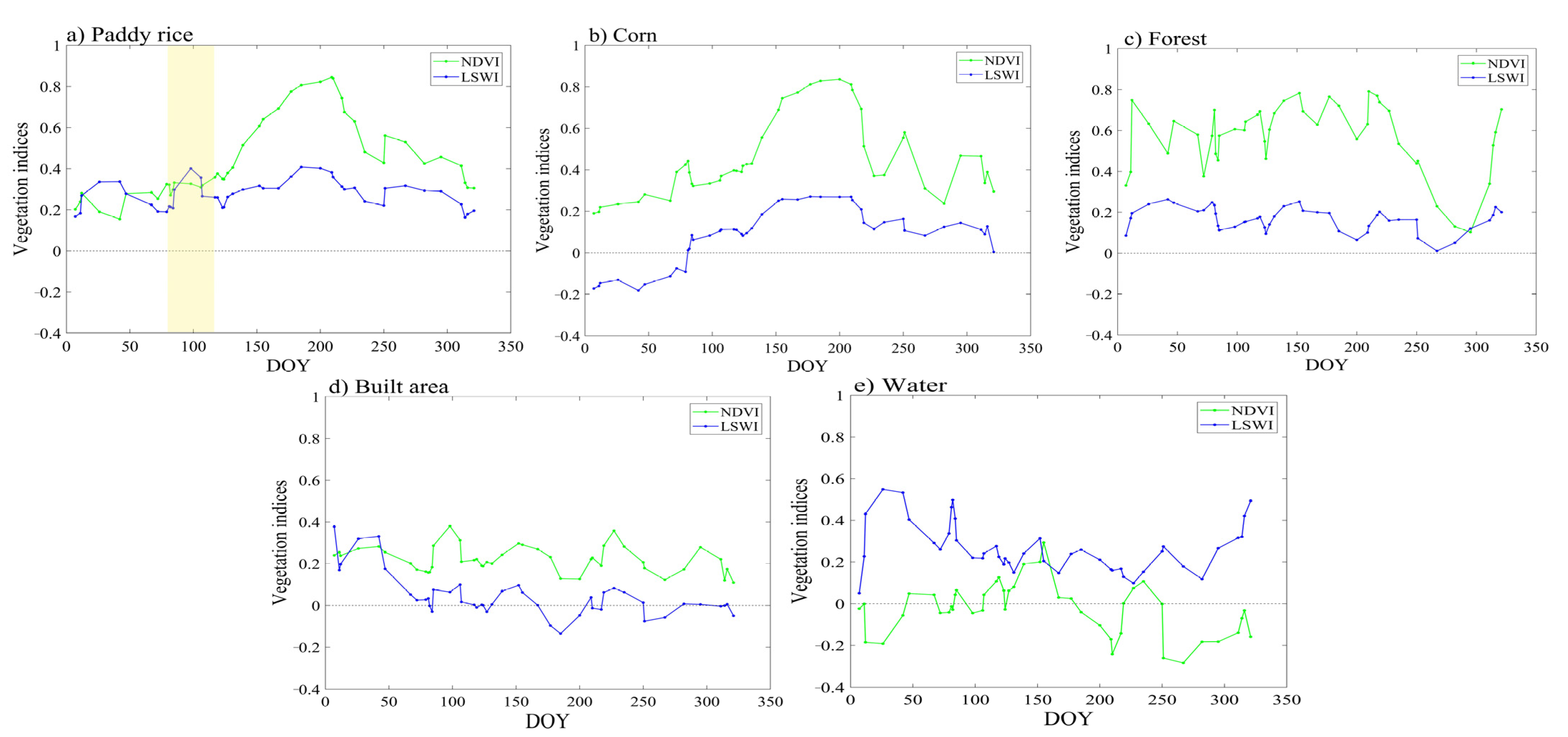
We smoothed NDVI and LSWI time series by Savitzky–Golay filter [32]. All the curves in Figure 5 are the results after smoothing. During the flooding period, the paddy rice fields were a mixture of water and green paddy rice plants, and the LSWI value was greater than the NDVI value (Figure 5a, ~DOY100). After transplanting the paddy rice seedlings, the NDVI of the paddy rice field gradually increased, and the LSWI gradually decreased. After transplanting, at about 80–100 days, most of the paddy rice fields were completely covered by the paddy rice canopy, and the LSWI value was lower than the NDVI value. The unique spectral feature of the flooded period (LSWI > NDVI) was used as a spectral signal to extract paddy rice when analyzing the time series satellite images [8,9,11]. In this study, we continued to explore algorithms that combine NDVI and LSWI. As shown in Figure 5a, the LSWI value was slightly higher than that of NDVI in the highlighted area, which was around DOY100. According to the previous phenological data, this period was the transplanting flood period. For fused images, we used the following threshold in the specific time window (DOY100 to DOY110) to identify flooded pixels: LSWI+0.1 $\ge$ NDVI. After a pixel is identified as having a transplanting signal, to ensure accuracy, follow-up changes in NDVI can be observed. Paddy rice crops grew rapidly after transplanting, and NDVI reached its peak (NDVI > 0.5) from DOY200 to DOY210.

3.3.2. Generating Other Land Cover Masks to Reduce Potential Impacts

Affected by factors such as atmospheric conditions and other land cover types with similar characteristics, the preliminary paddy rice map was inevitably polluted by noise [28]. Therefore, according to the phenology characteristics of other land cover types in the study area and the time distribution of VIs (Figure 5) [8,9,11,28,33], a mask was established to remove these noises to minimize their potential impact, as described below.

Crops in the non-flooded period (such as corn) and forest vegetation had LSWI < NDVI during the entire observation period, and the curve changes had similar trends (Figure 5b,c). In this study, we divided the pixels whose LSWI values were always less than the NDVI values during the growing season into crops in the non-flooded period and forests. The built area had an LSWI < 0 value throughout the plant growing season (Figure 5d), and the pixels whose LSWI average was about 0 were divided into the built area. There was a unique relationship between LSWI and NDVI of permanent water pixels, that is, LSWI > NDVI, as shown in Figure 5e. In this study, we used pixels with an average NDVI < 0.1 during the entire observation period to be classified as permanent water bodies.

Finally, we combined the set threshold with the existing land cover type map to build a paddy rice map based on pixels.

3.4. Accuracy Assessment

3.4.1. Evaluation of the MNSPI Approach and the FSDAF Model

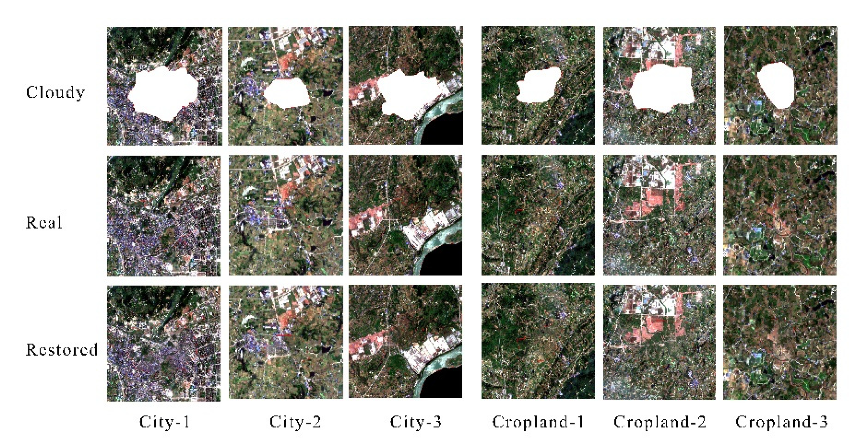
For the accuracy evaluation of the MNSPI method, we evaluated the accuracy of the MNSPI by comparing the cloud-removed images after randomly setting cloud patches with the original images [15]. For the Sentinel-2 images on 26 April and Landsat 8 OLI images on 2 May, in each image, we randomly designed three cloud patches for each land type to test the accuracy of the method under different land types. After the cloud removal process, we compared the reflectance values of restored pixel with the reflectance values of original images in the cloud patch.

For the accuracy evaluation of the FSDAF model, we evaluated the accuracy of FSDAF prediction by comparing the image predicted by FSDAF with the original image [24]. We used a Sentinel-2 image from 12 January and the MODIS images from 12 January and 26 April to predict a Sentinel-2 image from 26 April, and then we compared the predicted Sentinel-2 image on April 26 with the original Sentinel-2 image for evaluation.

The correlation coefficient (r) and root mean square error (RMSE) values of the predicted reflectance were compared with the true reflectance (including blue, green, red, near-infrared, SWIR band, NDVI, and LSWI) to quantitatively evaluate the accuracy [24]; r was used to show the linear relationship between predicted and actual reflectance. The closer the value of r is to one, the higher the consistency between the fused image and the original value. RMSE was used to measure the difference between the fusion image and the original image. The smaller the value, the smaller the difference between the fusion image and the original image, and the better the prediction effect. In addition to the comparison of reflectivity, the vegetation index was also compared accordingly. The RMSE calculation formula is as follows:

$$RMSE\left(F,G\right)=\frac{1}{B}{{\displaystyle \sum }}_{b=1}^B\sqrt{\frac{\parallel F_b-G_b\parallel {}^2}{N_1{N}_2}}$$

(4)

F and G represent the fusion image and the original image, respectively; b is the band number; and B is the total number of bands. $N_1{N}_2$ is the image size.

3.4.2. Accuracy Assessment of Paddy Rice Map

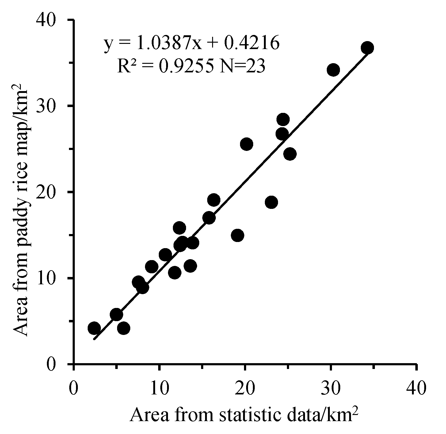
There are two ways to verify the paddy rice map. The first is to use field survey points for accuracy verification and calculate the overall accuracy and the Kappa coefficient. The second is to calculate the consistency of the paddy rice planting area with the official statistics.

4. Results

4.1. Accuracy of the MNSPI Approach and the FSDAF Model

Figure 6 shows the result of Sentinel-2 using cloudless image simulation on 26 April to remove the clouds. Figure 7 shows the result of Landsat 8 OLI’s cloud image de-cloud simulation using cloudless images on 2 May. It can be seen that MNSPI approach can restore most of the image features covered by thick clouds and shadows. However, the small boundaries (roads) on the image under the clouds are poorly restored, lacking continuity, and the boundaries are not obvious. In general, the performance of the MNSPI approach is not bad; the RMSE value of each type of land is small and the r value is high, which maintains the consistency of the images before and after cloud removal (

Table 2. RMSE and r values of the Sentinel-2 images before and after cloud removal.

Land Use	Sample	RMSE	r	Mean RMSE	Mean r
Cropland	cropland1	0.0136	0.9724	0.0135	0.9731
	cropland2	0.0140	0.9736
	cropland3	0.0128	0.9734
Water	water1	0.0064	0.9778	0.0144	0.9566
	water2	0.0261	0.9079
	water3	0.0108	0.9842
City	city1	0.0200	0.9466	0.0223	0.9554
	city2	0.0172	0.9592
	city3	0.0297	0.9604
Forest	forest1	0.0091	0.9817	0.0098	0.9785
	forest2	0.0086	0.9829
	forest3	0.0117	0.9711
Grassland	grassland1	0.0101	0.9866	0.0092	0.9883
	grassland2	0.0068	0.9945
	grassland3	0.0106	0.9840

and

Table 3. RMSE and r values of the Landsat 8 OLI images before and after cloud removal.

Land Use	Sample	RMSE	r	Mean RMSE	Mean r
Cropland	cropland1	0.0364	0.9981	0.0490	0.9964
	cropland2	0.0602	0.9949
	cropland3	0.0505	0.9963
Water	water1	0.0289	0.9987	0.0611	0.9894
	water2	0.0397	0.9972
	water3	0.1148	0.9725
City	city1	0.0399	0.9980	0.0760	0.9818
	city2	0.0480	0.9964
	city3	0.1401	0.9811
Forest	forest1	0.0364	0.9982	0.0350	0.9982
	forest2	0.0315	0.9985
	forest3	0.0371	0.9980
Grassland	grassland1	0.0371	0.9983	0.0555	0.9952
	grassland2	0.0541	0.9963
	grassland3	0.0754	0.9910

). In terms of different land types, the effect of cloud removal and restoration for forest, cropland, and grassland is better. The land type is uniform, and the method has good applicability.

Figure 8d shows the Sentinel-2-like image predicted by FSDAF on 26 April 2020. We used the enlarged area to highlight the difference between the predicted image and the actual image (Figure 8d,e). From a visual comparison point of view, the predicted image is basically similar to the original Sentinel-2 image, indicating that the method can capture the reflectance change of the land cover from 11 January 2020 to 26 April 2020. For all five bands, the RMSE values of the fusion results of FSDAF were small, and the r values were also high. The average RMSE value was 0.0246, and the average r value was 0.9417 (

Table 4. Accuracy assessment of the FSDAF model applied to the simulated dataset.

Band	RMSE	r	Indices	RMSE	r
Blue	0.0133	0.9287	NDVI	0.1002	0.9381
Green	0.0142	0.9566	LSWI	0.0791	0.7318
Red	0.0177	0.9274
NIR	0.0462	0.9435
SWIR	0.0316	0.9521
Multiband	0.0246	0.9417

), indicating that the FSDAF’s prediction was accurate. For vegetation indices (NDVI and LSWI), the RMSE value was small, and the prediction result was better. However, for r, NDVI was significantly better than LSWI. The r value of NDVI was 0.9381, and the r value of LSWI was 0.7318 There are many reasons for the different correlations between the two indexes, which may be related to factors such as wavebands and image land cover types [34]. Although the r value of LSWI was not enough, it was within the acceptable range. The accuracy evaluation results show that the FSDAF fusion image had a high correlation with the actual Sentinel-2 image (r = 0.9417, RMSE = 0.0246). Therefore, the fused image is reliable for the accuracy of subsequent research.

4.2. Fused Time Series Data

In this study, Sentinel-2, Landsat 8 OLI, and MOD09GA were used as optical remote sensing data sources, and the MNSPI cloud removal method and FSDAF spatiotemporal fusion method were used to construct the fused time series remote sensing data of the study area (Figure 9). First, after preprocessing Sentinel-2 and Landsat 8 OLI images, the MNSPI approach was used to perform cloud removal and interpolation processing on the images with more cloud coverage. Sentinel-2 had a total of eight images for cloud removal, and Landsat 8 OLI had a total of six images. After this, the MOD09GA images were fused. The number of MOD09GA images was selected on the basis of the existing Sentinel-2 and Landsat 8 OLI to supplement the missing images in the time series. The FSDAF algorithm was used to predict Sentinel-2-like images based on MOD09GA. MOD09GA selected a total of 16 images for FSDAF fusion to generate 16 Sentinel-2 images. For the Landsat8 OLI images, because its resolution is 30 m, it can basically meet the research needs. There was no FSDAF fusion for this, just resampled to 10 m using triple cubic convolution method [35]. Finally, we obtained the fusion time series data of the study area (Figure 9), a total of 44 images. The spatial resolution was 10 m. The temporal resolution of the data was controlled within 5 to 16 days.

4.3. Paddy Rice Map and Accuracy Assessment

According to the time series data and phenology method to generate a distribution map of the paddy rice planting area of 10 m in study area (Figure 10), paddy rice is distributed throughout the region, with more planted areas in the south than in the north. There are many paddy fields distributed in contiguous areas, and large paddy fields have different shapes (Figure 10). Paddy rice fields are mainly distributed in plain areas and along the rivers. Most of the paddy rice fields are located in areas with flat terrain and low elevation. The paddy rice fields are far away from the central urban area of Yongchuan District, and the town-level paddy rice fields are mostly distributed around the crowded areas. Farm roads are built in the farmland areas, and the planting personnel have convenient transportation. In Figure 10, paddy rice extraction results of six randomly selected regions are compared with the original images. It can be seen that edge and background of the 10 m resolution Sentinel-2 data have a high degree of matching. The extraction results are basically in line with the actual situation. However, due to the pixel-based method for extraction, a “salt and pepper” effect is inevitable.

After summarizing, the paddy rice planting area in Yongchuan District of Chongqing City is 382.03 square kilometers, which is close to the statistical data. The field survey points were divided into two types of paddy rice and non-paddy rice, and a confusion matrix was established to evaluate the accuracy of the results obtained. The confusion matrix is shown in

Table 5. Confusion matrix of paddy rice planting area map and field survey points.

Class	Ground Truth Pixels		Total	Consumer’s Accuracy
	Paddy Rice	Non-Paddy Rice
Paddy rice	274	15	289	95%
Non-paddy rice	23	199	222	90%
Total	297	214	511
Producer’s accuracy	92%	93%
Overall accuracy	93%
Kappa coefficient	0.85

. A total of 297 paddy rice samples were used for verification, of which 23 were misclassified. A total of 214 samples were used for verification of other types of land, with 15 misclassifications. The Kappa coefficient is 0.85. According to the data of the third national land survey, the area of paddy rice fields in each town in Yongchuan District was calculated.

Table 6. Comparison of the paddy rice area map and official statistics at the town and street level.

Town/Street	Statistic Data/km2	Classification Result/km2	Town/Street	Statistic Data/km2	Classification Result/km2
Banqiao	12.41	13.79	Qingfeng	12.7	14.13
Baofeng	10.71	12.69	Sanjiao	24.43	28.41
Chashanzhuhai	5.84	4.16	Shengli Road	9.11	11.31
Chenshi	25.23	24.39	Shuangshi	13.61	11.4
Daan	23.07	18.79	Songgai	5	5.76
Hegeng	20.18	25.54	Weixing Lake	12.34	15.81
Honglu	11.8	10.62	Wujian	8.04	8.9
Jian	13.88	14.08	Xianlong	24.32	26.73
Jinlong	15.79	16.98	Yongrong	7.58	9.51
Laisu	30.29	34.15	Zhongshan Road	2.4	4.16
Linjiang	19.12	14.95	Zhutuo	34.26	36.71
Nandajie	16.35	19.06

and Figure 11 compare the final paddy rice map with official statistics. The agreement is good, reaching a correlation of 92.5% at the town level. The good match between the paddy rice area based on the time series fusion data and the official statistical data clearly shows the accuracy of the final classification results. The above results show that the paddy rice extraction method based on spatiotemporal data fusion and the phenology-based method is stable and reliable in the cloudy and rainy Yongchuan District and can effectively distinguish between paddy rice and non-paddy rice areas.

5. Discussion

It is difficult to obtain sufficiently clear optical images with high spatiotemporal resolution in cloudy and rainy areas. Therefore, the ultimate goal of this research was to provide an operational method for paddy rice mapping by alleviating or avoiding data limitations to a certain extent. In this study, the MNSPI approach and the FSDAF model were used to obtain high-precision time series data, as well as a new method combined with a phenology-based algorithm. The study results show that the accuracy of this method is better. The MNSPI approach and the FSDAF model both had high accuracy, and the reflectivity of the predicted image was consistent with the original image. The final paddy rice map accuracy verification result was also good, and there was a good correlation with the official data. In addition, the two models had a high degree of automation. Users only need to prepare basic input data and modify a few parameters to run the program [15]. On the whole, the method used in this study has a good application effect in cloudy and rainy areas.

The method proposed in this study still has certain limitations: First, in the process of applying the MNSPI approach, as cloud cluster size increases, the accuracy of the restored image decreases slightly. This is because this method uses cloud neighborhood information. The larger the area of the cloud, the farther the distance between the target pixel and its similar pixels, the correlation may decrease, and therefore prediction accuracy may decrease. Furthermore, in areas with frequent and persistent clouds, it is difficult to reconstruct image time series with acceptable accuracy because clouds completely cover many images [15]. Second, generally speaking, the prediction quality of Sentinel-2-like images is affected by the time interval between base image date ($t_1$) and predicted image date ($t_2$). The longer the time interval, the worse the quality of the FSDAF-predicted image [24]. In our study, the time interval was controlled within 90 days. In addition, the accuracy of the input image in the FSDAF model will also affect the prediction results. After removing the cloud for input image, the number of effective pixels in the image will affect the prediction accuracy of the model to a certain extent. One problem common to the two methods above is that both methods have similar pixel search processes, and therefore a long calculation time may be required when processing large areas of massive images. Therefore, when rebuilding time series in a large area and long period, it is recommended to use a high-performance computer or cloud platforms to increase the calculation speed, for example, Pei Engine and Google Earth Engine [36]. Third, we used a pixel-based method for classification. The land types in the study area were relatively fragmented, and as a result, the “salt and pepper” effect inevitably appears. It can be seen from the example in Figure 10 that, in a small area, the same types of features were classified into different categories, and the originally uniform plot was divided into many blocks. There was also the problem of mixed pixels. In the process of field collection, it was found that some paddy rice fields were too small in area and formed mixed pixels with other land cover (such as corn) [26,37]. Fourth, due to different phenological periods, the method proposed in this study may not be directly applicable to other regions. When it is applied to other regions, it is necessary to carefully review and select the threshold value of paddy rice detection indicators.

Some studies have shown that because SAR data are not affected by weather conditions, SAR data have better application prospects in areas with clouds and fog [38]. Studies have also proven that the combination of optical and SAR data can improve the extraction accuracy of land cover information in areas with severe heterogeneity [39,40]. In addition, object-based image analysis (OBIA) technology continues to develop and has been successfully applied in many fields. It can reduce the occurrence of the salt and pepper phenomenon. In high-spatial resolution remote sensing images, especially the mapping of fragmented paddy rice fields, object-based classification methods are more advantageous than pixel-based classification methods [26,37]. Therefore, subsequent paddy rice mapping methods in cloudy and rainy areas can consider the fusion of SAR data and optical data and the use of object-based methods to improve the accuracy of the results.

6. Conclusions

Due to complicated observation conditions and the low number of effective optical remote sensing images in cloudy and rainy areas, it is difficult to map paddy rice fields for them. In this study, we propose a paddy rice mapping method based on spatiotemporal data fusion and a phenology-based algorithm. In this study, the MNSPI cloud removal method and the FSDAF spatiotemporal fusion model were used to construct time series data of the study area. The classification was based on the NDVI and LSWI change indicators in the key stages of phenology and combined with other auxiliary data to improve the accuracy of the results. Finally, we constructed fusion data with a spatial resolution of 10 m and a temporal resolution from 5 to 16 days. The distribution map of paddy rice planting areas was verified, and the overall accuracy was 93%, and the Kappa coefficient was 0.85. The paddy rice planting area map was also consistent with the official data of the third national land survey. At the town level, the correlation was 92.5%. The results prove the effectiveness of the method in cloudy and rainy areas. With the opportunity provided by the spatiotemporal fusion method, the method proposed in this study can provide a reference of certain significance for paddy rice surveying and mapping in cloudy rain areas. Our future work will consider fusing optical and radar data, using object-based and machine learning methods, and using cloud computing platforms to improve computational efficiency to provide more effective methods for monitoring crop type in cloudy and rainy areas.

References

1. Kuenzer, C.; Knauer, K. Remote sensing of rice crop areas. Int. J. Remote Sens. 2013, 34, 2101–2139. [Google Scholar] [CrossRef]
2. Gilbert, M.; Golding, N.; Zhou, H.; Wint, G.R.; Robinson, T.P.; Tatem, A.J.; Lai, S.; Zhou, S.; Jiang, H.; Guo, D.; et al. Predicting the risk of avian influenza A H7N9 infection in live-poultry markets across Asia. Nat. Commun. 2014, 5, 4116. [Google Scholar] [CrossRef] [PubMed] [Green Version]
3. Hongo, C.; Sigit, G.; Shikata, R.; Tamura, E. Estimation of water requirement for rice cultivation using satellite data. In Proceedings of the 2015 IEEE International Geoscience and Remote Sensing Symposium (IGARSS), Milan, Italy, 26–31 July 2015. [Google Scholar]
4. Sass, R.L.; Cicerone, R.J. Photosynthate allocations in rice plants: Food production or atmospheric methane? Proc. Natl. Acad. Sci. USA 2002, 99, 11993–11995. [Google Scholar] [CrossRef] [PubMed] [Green Version]
5. van Vliet, J.; Eitelberg, D.A.; Verburg, P.H. A global analysis of land take in cropland areas and production displacement from urbanization. Glob. Environ. Chang. 2017, 43, 107–115. [Google Scholar] [CrossRef]
6. Zhao, R.; Li, Y.; Ma, M. Mapping Paddy Rice with Satellite Remote Sensing: A Review. Sustainability 2021, 13, 503. [Google Scholar] [CrossRef]
7. Gumma, M.K.; Mohanty, S.; Nelson, A.; Arnel, R.; Mohammed, I.A.; Das, S.R. Remote sensing based change analysis of rice environments in Odisha, India. J. Environ. Manag. 2015, 148, 31–41. [Google Scholar] [CrossRef] [Green Version]
8. Xiao, X.; Boles, S.; Liu, J.; Zhuang, D.; Frolking, S.; Li, C.; Salas, W.; Moore, B. Mapping paddy rice agriculture in southern China using multi-temporal MODIS images. Remote Sens. Environ. 2005, 95, 480–492. [Google Scholar] [CrossRef]
9. Qin, Y.; Xiao, X.; Dong, J.; Zhou, Y.; Zhu, Z.; Zhang, G.; Du, G.; Jin, C.; Kou, W.; Wang, J.; et al. Mapping paddy rice planting area in cold temperate climate region through analysis of time series Landsat 8 (OLI), Landsat 7 (ETM+) and MODIS imagery. ISPRS J. Photogramm. Remote Sens. 2015, 105, 220–233. [Google Scholar] [CrossRef] [Green Version]
10. Kontgis, C.; Schneider, A.; Ozdogan, M. Mapping rice paddy extent and intensification in the Vietnamese Mekong River Delta with dense time stacks of Landsat data. Remote Sens. Environ. 2015, 169, 255–269. [Google Scholar] [CrossRef]
11. Xiao, X.; Boles, S.; Frolking, S.; Li, C.; Babu, J.Y.; Salas, W.; Moore, B. Mapping paddy rice agriculture in South and Southeast Asia using multi-temporal MODIS images. Remote Sens. Environ. 2006, 100, 95–113. [Google Scholar] [CrossRef]
12. Zhang, G.; Xiao, X.; Dong, J.; Kou, W.; Jin, C.; Qin, Y.; Zhou, Y.; Wang, J.; Menarguez, M.A.; Biradar, C. Mapping paddy rice planting areas through time series analysis of MODIS land surface temperature and vegetation index data. ISPRS J. Photogramm. Remote Sens. Off. Publ. Int. Soc. Photogramm. Remote Sens. 2015, 106, 157–171. [Google Scholar] [CrossRef] [Green Version]
13. Dong, J.; Xiao, X.; Kou, W.; Qin, Y.; Zhang, G.; Li, L.; Jin, C.; Zhou, Y.; Wang, J.; Biradar, C.; et al. Tracking the dynamics of paddy rice planting area in 1986–2010 through time series Landsat images and phenology-based algorithms. Remote Sens. Environ. 2015, 160, 99–113. [Google Scholar] [CrossRef]
14. Whyte, A.; Ferentinos, K.P.; Petropoulos, G.P. A new synergistic approach for monitoring wetlands using Sentinels -1 and 2 data with object-based machine learning algorithms. Environ. Modell Softw. 2018, 104, 40–54. [Google Scholar] [CrossRef] [Green Version]
15. Zhu, X.; Gao, F.; Liu, D.; Chen, J. A Modified Neighborhood Similar Pixel Interpolator Approach for Removing Thick Clouds in Landsat Images. IEEE Geosci. Remote Sens. Lett. 2012, 9, 521–525. [Google Scholar] [CrossRef]
16. Benabdelkader, S.; Melgani, F. Contextual Spatiospectral Postreconstruction of Cloud-Contaminated Images. Geosci. Remote Sens. Lett. IEEE 2008, 5, 204–208. [Google Scholar] [CrossRef]
17. Helmer, E.H.; Ruefenacht, B. Cloud-free satellite image mosaics with regression trees and histogram matching. Photogramm. Eng. Remote Sens. 2005, 71, 1079–1089. [Google Scholar] [CrossRef] [Green Version]
18. Melgani, F. Contextual reconstruction of cloud-contaminated multitemporal multispectral images. IEEE Trans. Geosci. Remote Sens. 2006, 44, 442–455. [Google Scholar] [CrossRef]
19. Meng, Q.M.; Borders, B.E.; Cieszewski, C.J.; Madden, M. Closest Spectral Fit for Removing Clouds and Cloud Shadows. Photogramm. Eng. Remote Sens. 2009, 75, 569–576. [Google Scholar] [CrossRef] [Green Version]
20. Chen, J.; Zhu, X.; Vogelmann, J.E.; Gao, F.; Jin, S. A simple and effective method for filling gaps in Landsat ETM + SLC-off images. Remote Sens. Environ. 2011, 115, 1053–1064. [Google Scholar] [CrossRef]
21. Hilker, T.; Wulder, M.A.; Coops, N.C.; Seitz, N.; White, J.C.; Gao, F.; Masek, J.G.; Stenhouse, G. Generation of dense time series synthetic Landsat data through data blending with MODIS using a spatial and temporal adaptive reflectance fusion model. Remote Sens. Environ. 2009, 113, 1988–1999. [Google Scholar] [CrossRef]
22. Zhao, Y.; Huang, B.; Song, H. A robust adaptive spatial and temporal image fusion model for complex land surface changes. Remote Sens. Environ. 2018, 208, 42–62. [Google Scholar] [CrossRef]
23. Zhu, X.; Chen, J.; Gao, F.; Chen, X.; Masek, J.G. An enhanced spatial and temporal adaptive reflectance fusion model for complex heterogeneous regions. Remote Sens. Environ. 2010, 114, 2610–2623. [Google Scholar] [CrossRef]
24. Zhu, X.; Helmer, E.H.; Gao, F.; Liu, D.; Chen, J.; Lefsky, M.A. A flexible spatiotemporal method for fusing satellite images with different resolutions. Remote Sens. Environ. 2016, 172, 165–177. [Google Scholar] [CrossRef]
25. Zhu, L.; Radeloff, V.C.; Ives, A.R. Improving the mapping of crop types in the Midwestern U.S. by fusing Landsat and MODIS satellite data. Int. J. Appl. Earth Obs. Geoinf. 2017, 58, 1–11. [Google Scholar] [CrossRef]
26. Zhang, M.; Lin, H. Object-based rice mapping using time-series and phenological data. Adv. Space Res. 2019, 63, 190–202. [Google Scholar] [CrossRef]
27. Cai, Y.; Lin, H.; Zhang, M. Mapping paddy rice by the object-based random forest method using time series Sentinel-1/Sentinel-2 data. Adv. Space Res. 2019, 64, 2233–2244. [Google Scholar] [CrossRef]
28. Yin, Q.; Liu, M.; Cheng, J.; Ke, Y.; Chen, X. Mapping Paddy Rice Planting Area in Northeastern China Using Spatiotemporal Data Fusion and Phenology-Based Method. Remote Sens. 2019, 11, 1699. [Google Scholar] [CrossRef] [Green Version]
29. Karra, K.; Kontgis, C.; Statman-Weil, Z.; Mazzariello, J.C.; Mathis, M.; Brumby, S.P. Global land use/land cover with Sentinel-2 and deep learning. In Proceedings of the IGARSS 2021–2021 IEEE International Geoscience and Remote Sensing Symposium, Brussels, Belgium, 11–16 July 2021. [Google Scholar]
30. Zhu, X.; Helmer, E.H.; Chen, J.; Liu, D. An automatic system for reconstructing High-quality seasonal Landsat time series. In Remote Sensing Time Series Image Processing; Weng, Q., Ed.; Taylor and Francis Series in Imaging Science; CRC Press: Boca Raton, FL, USA, 2018; pp. 25–42. [Google Scholar]
31. Xiao, X.; Boles, S.; Frolking, S.; Salas, W.; Moore, B.; Li, C.; He, L.; Zhao, R. Landscape-scale characterization of cropland in China using Vegetation and landsat TM images. Int. J. Remote Sens. 2002, 23, 3579–3594. [Google Scholar] [CrossRef]
32. Chen, J.; Jönsson, P.; Tamura, M.; Gu, Z.; Matsushita, B.; Eklundh, L. A simple method for reconstructing a high-quality NDVI time-series data set based on the Savitzky–Golay filter. Remote Sens. Environ. 2004, 91, 332–344. [Google Scholar] [CrossRef]
33. Zhou, Y.; Xiao, X.; Qin, Y.; Dong, J.; Zhang, G.; Kou, W.; Jin, C.; Wang, J.; Li, X. Mapping paddy rice planting area in rice-wetland coexistent areas through analysis of Landsat 8 OLI and MODIS images. Int. J. Appl. Earth Obs. Geoinf 2016, 46, 1–12. [Google Scholar] [CrossRef] [Green Version]
34. Jarihani, A.; McVicar, T.; Van Niel, T.; Emelyanova, I.; Callow, J.; Johansen, K. Blending Landsat and MODIS Data to Generate Multispectral Indices: A Comparison of “Index-then-Blend” and “Blend-then-Index” Approaches. Remote Sens. 2014, 6, 9213–9238. [Google Scholar] [CrossRef] [Green Version]
35. Keys, R.G. Cubic Convolution Interpolation for Digital Image-Processing. IEEE T Acoust. Speech 1981, 29, 1153–1160. [Google Scholar] [CrossRef] [Green Version]
36. Pan, L.; Xia, H.; Zhao, X.; Guo, Y.; Qin, Y. Mapping Winter Crops Using a Phenology Algorithm, Time-Series Sentinel-2 and Landsat-7/8 Images, and Google Earth Engine. Remote Sens. 2021, 13, 2510. [Google Scholar] [CrossRef]
37. Yang, H.; Pan, B.; Wu, W.; Tai, J. Field-based rice classification in Wuhua county through integration of multi-temporal Sentinel-1A and Landsat-8 OLI data. Int. J. Appl. Earth Obs. Geoinf. 2018, 69, 226–236. [Google Scholar] [CrossRef]
38. Yun, S.; Fan, X.; Liu, H.; Xiao, J.; Ross, S.; Brisco, B.; Brown, R.; Staples, G. Rice monitoring and production estimation using multitemporal RADARSAT. Remote Sens. Environ. 2001, 76, 310–325. [Google Scholar]
39. Bazzi, H.; Baghdadi, N.; El Hajj, M.; Zribi, M.; Minh, D.H.T.; Ndikumana, E.; Courault, D.; Belhouchette, H. Mapping Paddy Rice Using Sentinel-1 SAR Time Series in Camargue, France. Remote Sens. 2019, 11, 887. [Google Scholar] [CrossRef] [Green Version]
40. Nguyen, D.; Clauss, K.; Cao, S.; Naeimi, V.; Kuenzer, C.; Wagner, W. Mapping Rice Seasonality in the Mekong Delta with Multi-Year Envisat ASAR WSM Data. Remote Sens. 2015, 7, 15868–15893. [Google Scholar] [CrossRef] [Green Version]
Figure 1. The location of the study area and its digital elevation model (DEM).
Remotesensing 13 04400 g001
Figure 2. Percentage chart of weather statistics in the study area in 2020 based on historical weather data from the China Meteorological Network.
Remotesensing 13 04400 g002
Figure 3. Spatial distribution of field survey data in the study area.
Remotesensing 13 04400 g003
Figure 4. A flow chart of the algorithm for mapping paddy rice area.
Remotesensing 13 04400 g004
Figure 5. The seasonal dynamics of NDVI and LSWI for the major land use types at selected sites, extracted from fused time series data: (a) Paddy rice; (b) corn; (c) forest; (d) built area; (e) water. All sites were selected from the field survey data.
Remotesensing 13 04400 g005
Figure 6. The red–green–blue composite images of Sentinel-2 image that were acquired on 26 April 2020. Three plots were selected for each land type. The cloud images in the first row are cloudy images simulated based on the real images in the second row. The third row is images recovered by the MNSPI approach. The white area represents the simulated thick cloud patch, and the red line is the cloud patch boundary.
Remotesensing 13 04400 g006aRemotesensing 13 04400 g006b
Figure 7. The red–green–blue composite images of Landsat 8 OLI image that were acquired on 2 May 2020. Three plots were selected for each land type. The cloud images in the first row are cloudy images simulated based on the real images in the second row. The third row is images recovered by the MNSPI approach. The white area represents the simulated thick cloud patch, and the red line is the cloud patch boundary.
Remotesensing 13 04400 g007
Figure 8. Images used for FSDAF verification: (a) Input data, coarse-resolution image, MODIS on 12 January; (b) input data, fine-resolution image, Sentinel-2 on 12 January; (c) input data, coarse-resolution image, MODIS on 26 April; (d) output data Sentinel-2-like image, on 26 April, predicted by FSDAF; (e) original Sentinel-2 image on 26 April. All images are displayed in true color and same size.
Remotesensing 13 04400 g008
Figure 9. Time distribution of each piece of data in fused time series data.
Remotesensing 13 04400 g009
Figure 10. Spatial distribution of paddy rice fields in Yongchuan District. Subplots: (af) represent the comparison between the detail map of paddy rice extraction results and remote sensing images in six randomly selected regions.
Remotesensing 13 04400 g010
Figure 11. Comparison of paddy rice map with official statistics.
Remotesensing 13 04400 g011