Article

Potential Temporal and Spatial Trends of Oceanographic Conditions with the Bloom of Ulva Prolifera in the West of the Southern Yellow Sea

1
Key Lab of Submarine Geosciences and Prospecting Techniques, MOE, OUC, Qingdao 266100, China
2
College of Marine Geoscience, Ocean University of China, Qingdao 266100, China
3
Qingdao Blue Earth Big Data Technology Company Limited, Qingdao 266400, China
4
College of Information Science and Engineering, Ocean University of China, Qingdao 266100, China
*
Author to whom correspondence should be addressed.
Remote Sens. 2021, 13(21), 4406; https://doi.org/10.3390/rs13214406
Submission received: 29 September 2021 / Revised: 23 October 2021 / Accepted: 30 October 2021 / Published: 2 November 2021

Abstract

:
Based on National Oceanic and Atmospheric Administration/Advanced Very High-Resolution Radiometer (NOAA/AVHRR) remote sensing and Cross-Calibrated Multi-Platform (CCMP) wind field data from 2007 to 2019, oceanographic conditions are analysed, respectively, in the Source Area (SA) and Typical Bloom Area (TBA) of Ulva prolifera (U. prolifera) in the west of the Southern Yellow Sea (SYS) using Sea Surface Temperature (SST), Suspended Sediment Concentration (SSC) and Wind Speed over the years. The results indicate that the annual maximum SST Difference (SSTD) between U. prolifera SA and TBA is strongly consistent with the intensity of U. prolifera, and a high SST Warming Rate (WR) from May to July may constrain the U. prolifera blooms. The Taiwan Warm Current (TWC), crossing Yangtze River Estuary northward from March to April, leads to SST increasing in the SA and becomes a key trigger for the growth of U. prolifera in the early period. The amount of U. prolifera may decrease in the early period because of the lower light intensity with high SSC and turbidity in SA. The summer monsoon is one of determinants for the spread of U. prolifera, and the distribution of U. prolifera reaches its highest point with a higher mean wind speed in the TBA.

1. Introduction

Since 2008, Enteromorpha in the west of Southern Yellow Sea (SYS) has bloomed and gathered in large numbers, and its presence has seriously affected coastal fisheries and tourism in Jiangsu and Shandong Province, becoming one of the most serious marine events in China [1]. The tongue-shaped topographical area (Figure 1a) off the coast of Northern Jiangsu in the west of the SYS covers a large area of shallow water, namely Subei Shoal, which is less than 20 m in depth. Thus, it serves as the largest Porphyra yezoensis breeding base in China. Studies indicate that the presence of Enteromorpha impacts that bloom in the SYS mostly originate along the laver breeding coast of Jiangsu Province [2,3,4], where the dominant species is Ulva prolifera (U. prolifera) [5]. This is because south-southeast wind prevails in the SYS in summer and the Sea Surface Temperature (SST) of 24~27 °C are within the suitable growth temperature interval of U. prolifera of 10~30 °C, which is the one of the main reasons why U. prolifera grows more and rapidly [6,7].
Previous papers have concluded that U. prolifera usually undergoes five stages (Table 1): origin, development, bloom, decline and extinction [8]. First, in April, U. prolifera is discovered in the sea area near Subei Shoal. Second, in mid-May, it takes shape in the sea area near Yancheng of Jiangsu Province, then drifts northward and develops continuously due to the leading role of the sea surface wind field. Third, in mid-to-late June, its largest coverage and distribution area is formed, and the northernmost part can reach the southern coast of Shandong Peninsula. Finally, its drift path is blocked by land, turns to northeast along the southern coast of Shandong Peninsula and gradually declines to extinction in mid-August. As a result, the bloom speed of U. prolifera is fast, the coverage area is large and the duration is long. There are large interannual differences in the origin location, origin time, duration, drift path and coverage area.
Limited by remote sensing and field data, previous studies have focused on the overall distribution of U. prolifera and the overall change of oceanographic conditions on a short timescale in the SYS [6,7,9,10,11,12,13]. However, the change of oceanographic conditions and its correlation to the bloom intensity, respectively, in different area of different stages have been ignored since the occurrence of U. prolifera impacted in the SYS in 2008. Based on Geo-stationary Ocean Color Imager (GOCI) data and the Normalized Difference Vegetation Index (NDVI) algorithm, Li et al. [7] extracted the distribution of U. prolifera in development, bloom and extinction period from 2011 to 2017; calculated the distribution density; and concluded that the overall trend of U. prolifera in SYS is “scattered development, clustered bloom, and diffused extinction.” Zhang et al. [11] used Huan Jing/Charge Coupled Device (HJ/CCD) data with high spatial resolution and Moderate-resolution Imaging Spectroradiometer (MODIS) data with high temporal resolution to analyse the origin environment and drift paths of U. prolifera from 2011 to 2017. Moreover, Sun et al. [12] established a quantitative relationship between MODIS and HJ/CCD data to extract U. prolifera based on the NDVI algorithm from 2011 to 2016. Previous studies have also shown that there is serious eutrophic activity in the SYS. As a result, the nutrients are sufficient in all stages of U. prolifera growth [14], and their change is not obvious before and after the U. prolifera impacts [15]. Therefore, the effect of nutrients is not discussed in this paper.
Although the presence of the U. prolifera event has occurred annually in different areas and different stages (Figure 1a) since 2008, interannual differences are large and influencing factors are complicated. The SST and sunlight intensity directly affect the origin and development of U. prolifera, and the wind field is the main driving factor. Therefore, this paper extracts the SST, Suspended Sediment Concentration (SSC) and wind field data from different areas where U. prolifera originates and blooms (Figure 1a) to investigate the multi-year changes in the oceanographic parameters since U. prolifera was first observed in the SYS in 2007. In addition, this paper analyses the comprehensive influence of oceanographic conditions on the bloom intensity of U. prolifera.

2. Data Sources and Methods
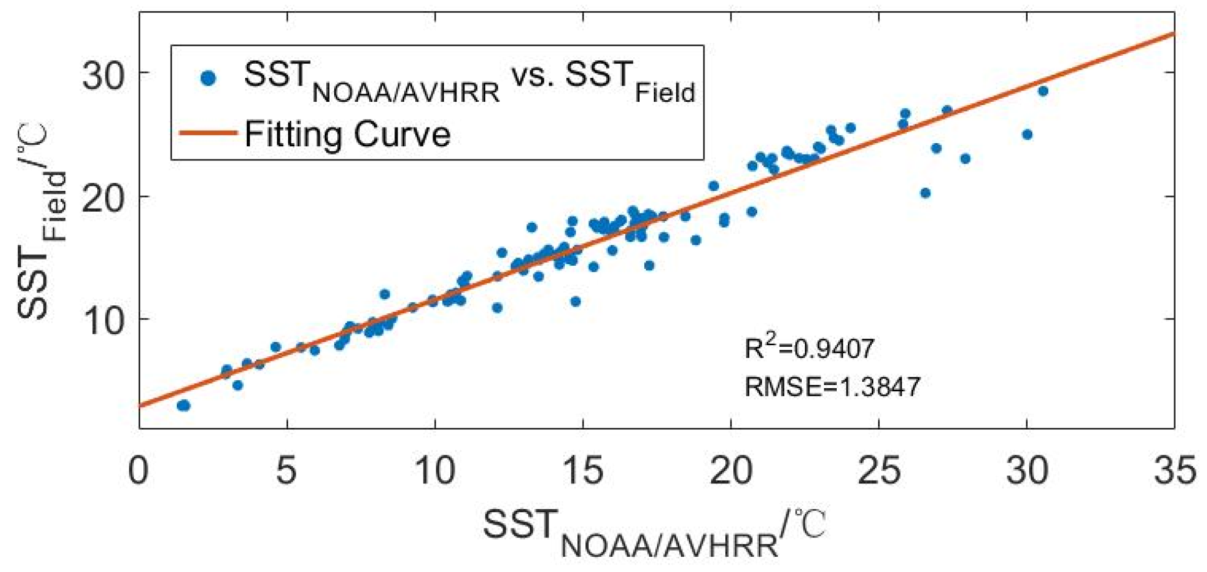
2.1. Data Sources

Multiple data are used in this paper (Table 2). The remote sensing data are from the third-generation Advanced Very High-Resolution Radiometer (AVHRR/3) provided by the National Oceanic and Atmospheric Administration (NOAA), with a resolution of 1.1 km [16,17,18].
Cross-Calibrated Multi-Platform (CCMP) sea surface wind field data are from the National Aeronautics and Space Administration’s (NASA) Physical Oceanography Distributed Active Archive Center (PO. DAAC), providing radial and zonal wind speed data 10 m above the sea surface with a horizontal resolution of 0.25° and a time interval of 6 h [19,20,21,22]. The data are updated to April 2019.
Field SST data are from National Natural Science Foundation of China (NSFC) Shiptime Sharing Project from 2010 to 2018, and the SST is measured by Conductivity-Temperature-Depth (CTD) of Sea-bird911. The stations are shown as yellow points in Figure 1a.
The data related to U. prolifera impacts supplemented in this paper are from Bulletin of China Marine Disaster (BCMD) [23,24,25], issued by the Ministry of Natural Resources of P.R.China from March to April every year. It has recorded, in detail, the earliest discovery location, maximum distribution time (date), Maximum Distribution Area (MDA), maximum coverage time (date), Maximum Coverage Area (MCA) and extinction time (date) of U. prolifera each year since 2009. These data are used to reflect the scale of U. prolifera event in Figure 7.

2.2. Methods

In this paper, ENVI/IDL 5.3 was used to pre-process NOAA/AVHRR (L1b) data, such as the radiometric correction, geometric correction, band math and cropping. After pre-processing, the albedo (in W/m2.μm.sr) was obtained through B1 (Visible Band with a wavelength of 0.58~0.68 μm) and B2 (Near-infrared Band with a wavelength of 0.727~1 μm), using the positive correlation between the albedo and SSC to reflect the distribution and diffusion of the SSC [26]. The SST was calculated from the calibrated brightness temperature of B3 (Mid-infrared Band with a wavelength of 1.58~3.93 μm), B4 (Thermal-infrared Band with a wavelength of 10.30~11.30 μm) and B5 (Thermal-infrared Band with a wavelength of 11.50~12.50 μm). The monthly mean SST and SSC were calculated by the daily data in every month after pre-processing. In addition, the SST Anomaly (SSTA) and SSC Anomaly (SSCA) were calculated by
SSTA = SST − month mean SST,
and
SSCA = SSC − month mean SSC.
Month mean refers to the mean value of each month of 13 years from 2007 to 2019.
The range of U. prolifera was identified by the NDVI [27]. The formula, based on the NOAA/AVHRR data, is:
NDVI = (Bnear-infrared − Bvisible)/(Bnear-infrared + Bvisible) = (B2 − B1)/(B2 + B1).
To determine the coverage area of U. prolifera, images with small cloud cover area in the study area were selected and processed by the NDVI algorithm after pre-processing. However, due to the influence of the spatial resolution and weather, the number of inversion images meeting the requirements of use was small. Since 2013, the effect of the NDVI algorithm has improved when the coverage of U. prolifera is relatively large (near maximum coverage date). Further research is still needed to extract the origin and distribution range of U. prolifera.

3. Results

Combining the SST based on NOAA/AVHRR with 124 effective field data, the SST inversion formula is:
SST = 0.867 × SSTNOAA/AVHRR + 2.8757,
and its R2 is 0.9407 (Figure 2).
Based on the data sources and methods in Section 2, the spatial pattern of the SST, SSC and wind field from 2007 to 2019 can be obtained (Figure 3).

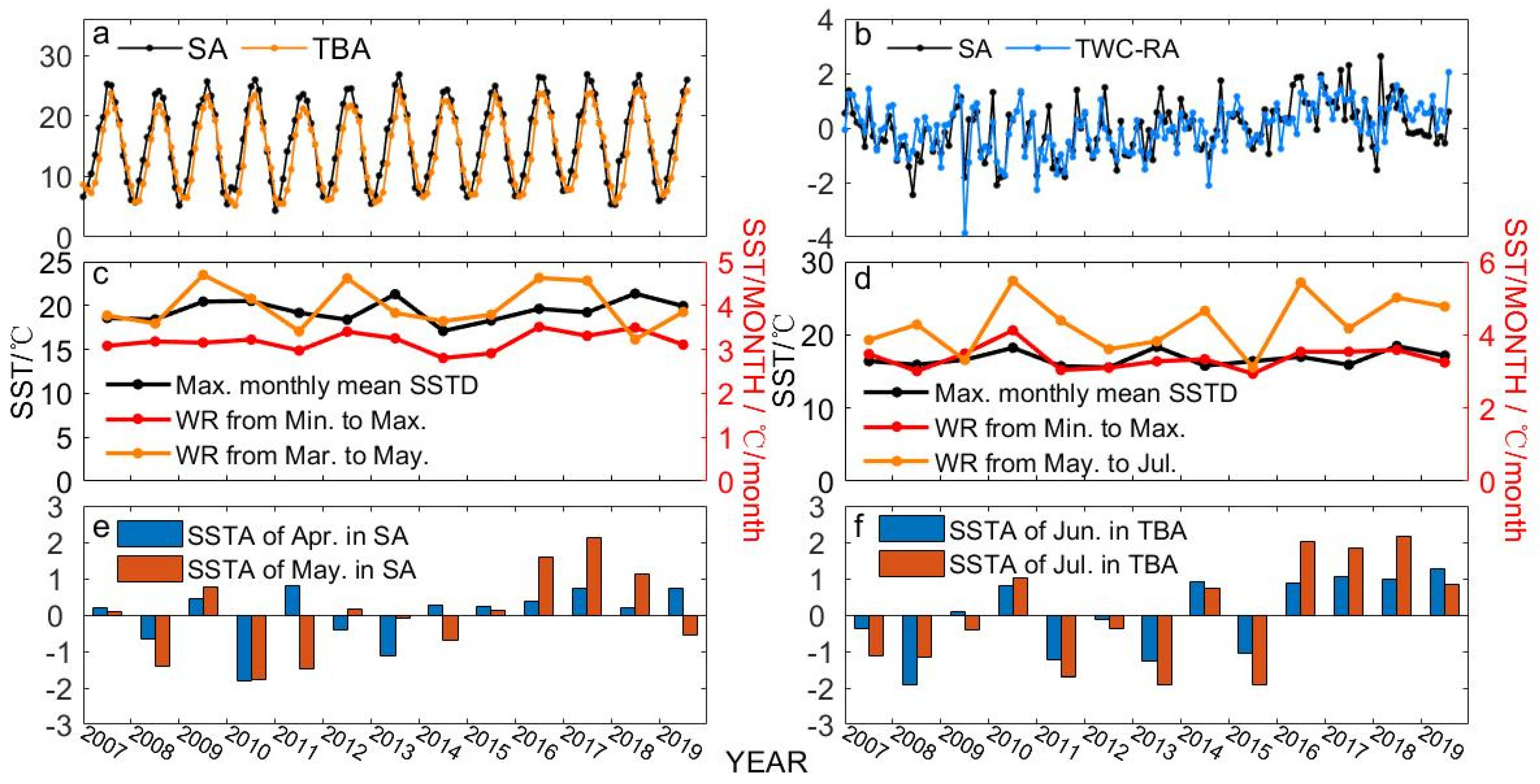
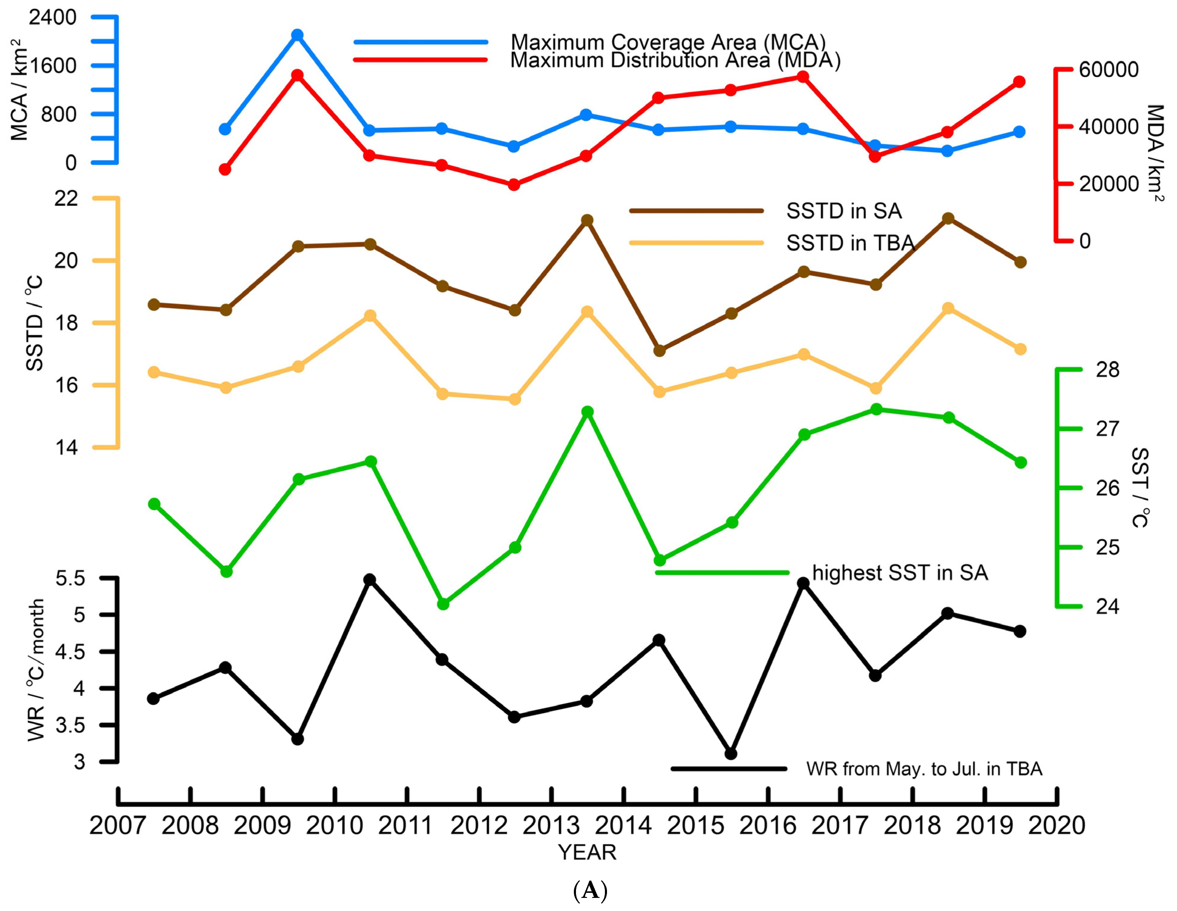
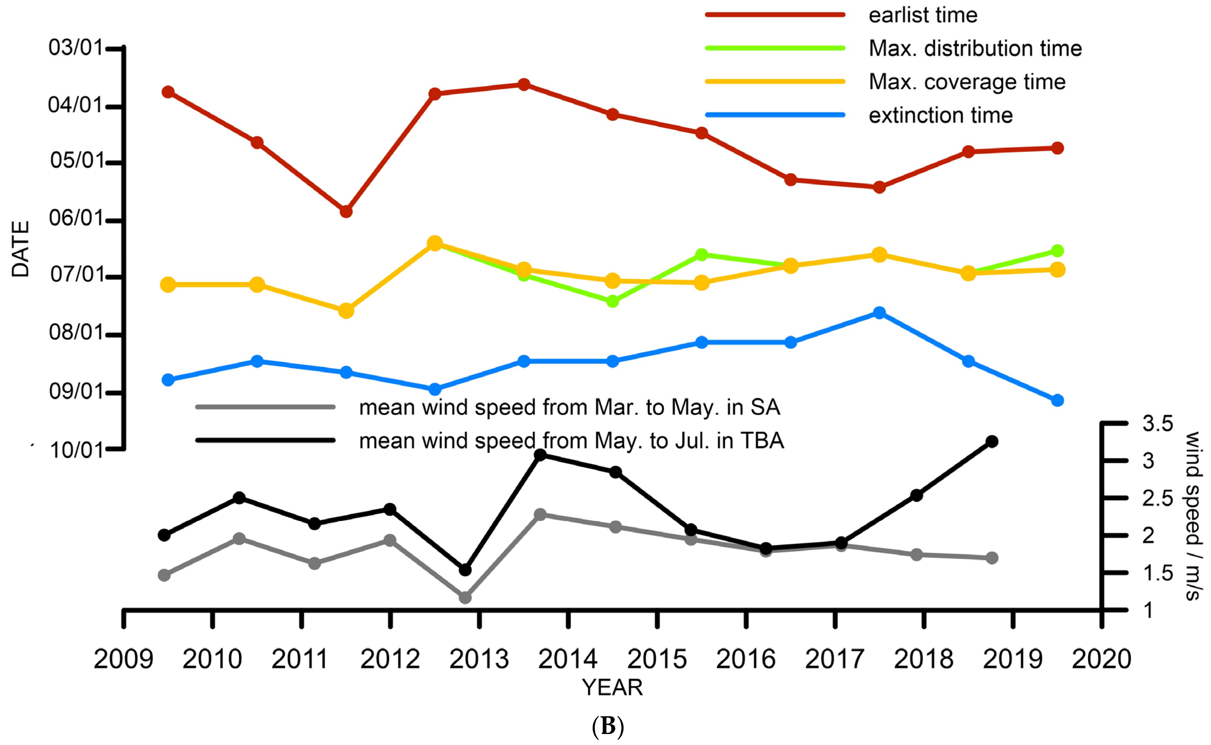
3.1. Sea Surface Temperature (SST)

On a timescale, the overall SST in the west of the SYS (Figure 3A) is in the warming phase from February to August, and the Warming Rate (WR) is relatively high from April to July. After July, the SST continues to rise, peaking in August, but the WR becomes slower. The SST begins to drop in September and reaches the lowest level in February of the next year. Spatially, the SST in the south of the SYS is significantly higher than that in the north from January to May and from October to December, and the SST in the coastal area is higher than that in the offshore area at the same latitude. In June, there is an obvious high-value centre in the north-central of the SYS, and the distribution of the SST in the SYS tends to be even from June to September, forming an SST equivalent zone. In addition, high-SST water tongue in the east coastal waters of Shanghai exceeds 32°N and extends northward to the east coastal waters of Yancheng in April, forming a U-shape with the high-SST waters of the open sea.
To analyse the impact of SST on the bloom intensity of U. prolifera in different areas and different stages, based on the NDVI remote sensing images and BCMD, this paper selects the northern sea area of Rudong in Jiangsu Province (32.4~32.9°N, 120.9~121.4°E) and the central of the SYS (35.1~35.6°N, 120.9~121.4°E) as the Source Area (SA) and Typical Bloom Area (TBA) of U. prolifera (Figure 1a), respectively. Based on NOAA/AVHRR data, the continuous change of monthly mean SST from 2007 to 2019 (Figure 4a) and the annual SST key parameters (Figure 4c,d) in two areas were calculated, respectively.
The SST in the SA (Figure 4a) is the lowest in January and the highest in August. The stage with the highest WR occurs from February to May. The SSTA in the SA from April to May (Figure 4e) was usually negative from 2010 to 2015 and positive after 2014. The SSTA in the TBA from June to July (Figure 4f) usually showed negative anomalies before 2015 and clear positive anomalies after 2015. The annual maximum SST underwent a cyclical increase, reaching the maximum point in 2010, 2013 and 2017. The SST from March to May and from the month of minimum SST to the month of maximum SST were selected to create scatterplots, respectively. The slope of fit line was taken as the SST WR, and the R2 of the fit lines were above 0.9. According to Figure 4c, the tWR from the minimum SST to maximum SST had a small range of change, with the highest in recent years in 2012. The annual variation of the SST WR in developing period of U. prolifera (March to May) was slightly higher than that of the WR from the minimum SST to maximum SST. There was a fast WR in 2009, 2012, 2016 and 2017, and a slow WR in 2008, 2011 and 2018.
In the TBA (Figure 4a), except for 2014 and 2016, which peaked in July, the lowest SST was in February and March, and the highest SST was in August. The period with the highest WR occurred from April to July. The annual maximum SST of the TBA presented a cyclical increase before 2013, and a slow rise since 2014. Using the same method, the fit WR from May to July and from the month of minimum SST to the month of maximum SST of each year was obtained (Figure 4d), and the R2 of fit lines were above 0.9. The WR from the minimum SST to maximum SST had a relatively small range of change, with the highest in recent years in 2010. The variation of the SST WR in development and bloom period of U. prolifera (Table 1) was significantly higher than that of WR from minimum SST to maximum SST. There was a fast WR in 2010, 2014, 2016 and 2018, and a slow WR in 2009, 2012, 2013, 2015 and 2017.
The SA and TBA of U. prolifera selected by remote sensing images have the same longitude range. Therefore, a transect from 121.2°E in the SA to the north was selected, and the monthly mean SST in the square area of 0.2° * 0.2° was counted at equal intervals (Figure 5A) to further analyse the temporal and spatial changes of the SST and its anomaly during the “origin-development-bloom” period of U. prolifera.
The isolines in Figure 5 are all SST isolines, including the 15 °C (gray line in Figure 5), 20 °C and 25 °C isotherms, respectively, showing the Temperature Window most suitable for the growth of U. prolifera [6,7]. At the 121.2°E transect (Figure 5A), the SST in the coastal area is higher than that in offshore area in the summer and lower in the winter, with a large variation range. On a timescale, the SST of 2010, 2013, 2016, 2017 and 2018 was greater in the summer. In addition, the SST of 2009, 2010, 2013 and 2018 in the winter was dramatically lower than that of other years. It indicates that the SST WR was higher in the diffusion path of U. prolifera in 2010, 2013 and 2018. The SST of the SYS in the summer has clearly risen along the diffusion path of U. prolifera since 2014. In the TBA near 35°N, the Temperature Window in 2011 and 2012 was significantly shorter than that in other years, and the Window period has significantly strengthened since 2016. In the Temperature Window most suitable for the growth of U. prolifera, the SST showed clear negative anamolies in 2008, 2011, 2014 and 2015, while the SST generally showed positive anamolies after 2016.

3.2. Suspended Sediment Concentration (SSC)

Turbidity affects the transparency of water and has a direct effect on the growth of U. prolifera. The SSC of the SYS (Figure 3B) is higher in the winter and lower in the summer. The SSC gradually decreases from January to May, increases slightly from May to June and then recovers the downward trend from June to September, reaching the lowest level in September. The SSC ascends rapidly from September to November, and then increases slowly after November, peaking in January of the next year. Spatially, the SSC is higher near the coast and lower offshore. There is a high-value centre located in Subei Shoal, and the south coast is slightly higher than north coast. The high-value centre begins to appear in the ancient Yellow River Estuary in October, peaking in December, then gradually moves southward and disappears in the southern sea area of Yancheng in April. In winter, there is also a small high-value centre in the southeast sea area of Shandong Peninsula.
To more accurately analyse whether the bloom intensity of U. prolifera has a direct response to the SSC, the continuous changes of the monthly mean SSC since 2007 were evaluated in the SA and TBA of U. prolifera based on the NOAA/AVHRR data (Figure 6).
The highest level of SSC in the SA (Figure 6a,c) appears from December to January of the next year, and the lowest level appears in July. The SSC increased in June after 2008. Since 2007, which had the annual maximum monthly mean SSC, the monthly mean SSC in April and May has shown an upward trend, and the increasing rate has gradually risen. Except for 2009 and 2011, the monthly mean SSC in April has been higher than that in May. The highest level of SSC in the TBA (Figure 6b,d) still appears in December to January of the next year, and the lowest level appears from August to September. Since 2007, the SSC has increased from April to August. The annual maximum SSC in the TBA and monthly mean SSC in June and July are all on upward cyclical trends. The monthly mean SSC in June was higher than that in July in 2009, 2011, 2015 and 2018, while it was higher in July in other years.
A transect from 121.2°E in the SA to the north was selected, and the monthly mean SSC in square area of 0.2° * 0.2° was calculated at equal intervals to analyse the temporal and spatial changes of the SSC and its anomaly during the “origin-development-bloom” stage of U. prolifera (Figure 5B). The SSC of the sea area north of 34°N was low, and the sea area south of 34°N was mainly the Subei Shoal area with a high SSC, forming a high-value centre near 33°N. On a timescale, there are usually two low-value centres in sea area north of 34°N in the summer half year, and the Temperature Window most suitable for U. prolifera growth in 2009 and 2011~2015 clearly corresponds to the second The SSC in the shoal area south of 34°N has ascended since 2015. The SSC in the summer of 2009, 2012 and 2013 was slightly lower than those in other years, and the SSC in the winter of 2010 and 2014 was significantly lower than those in other years. In 2013, there was a clear negative anomaly in the Temperature Window, while it was positive in 2014, 2017 and 2018.
The appropriate SST and lower SSC may lead to massive U. prolifera blooms. After 2014, both the SST and SSC in the SYS have shown increasing trends, though the reasons must be studied.

3.3. Wind Field

The wind field in the SYS (Figure 3C) shows typical seasonal variation and strong regional characteristics. In winter, there is a strong northwest wind. The wind is the strongest from December to January of the next year, and the maximum wind speed in the open sea can reach 6~7 m/s. From February to March, the wind field gradually weakens and turns north-easterly in the west of the SYS. In April, the wind field begins to turn to east-south wind, and the wind speed reaches the lowest level of the whole year. From May to July, during the “development-bloom-extinction” stage of U. prolifera, the wind direction turns to the southeast, and the twind speed also gradually increases. August is the second transitional month of the wind field in the SYS, as wind direction turns to east-southeast, and the wind speed weakens. From September to December, the wind direction gradually changes from northeast to northwest, and the wind speed continues to rise.
To further analyse the influence of the wind field on the SSC changes and U. prolifera during the “origin-development-bloom” stage, the continuous changes of monthly mean wind speed were calculated in the SA and the TBA of U. prolifera since 2007, respectively, based on CCMP data (Figure 6a,b). The wind speed changes in SA are relatively stable, peaking in winter, and the monthly mean wind speed also ascends when affected by multi-typhoon weather in the summer. Since 2008, the wind speed in the SA has peaked approximately at 5 m/s in autumn and winter (November to February of next year) with a 3-year interval. speed in the TBA has strong seasonal variation and also peaks in winter. Wind speed in the summer is less affected by the multi-typhoon weather than that in the SA. Wind speed in the winter of 2008, 2011 and 2015 peaks more than 6 m/s.

4. Discussion

Ulva species are notorious for their ability to form green tides, especially when they are in optimum oceanographic conditions around 30~40°N [28,29]. In the Gulf of California, Ulva species have a high presence and cover in late winter and spring, and a decreasing presence in the summer when the SST exceeds 25 °C [30]. Ulva is a widely distributed species that shows a broad tolerance to temperature, intensity of sunlight and wind field, which is evident as this species remains until the SST is above 30 °C.
In terms of the bloom area of U. prolifera (Figure 7A), since the first large-scale bloom in 2008, the MCA and MDA of U. prolifera both reached maximum in 2009, and there have been magnificent differences in interannual changes after 2010. Moreover, 2012 was the weakest year since the bloom of U. prolifera impacts, with the smallest MCA and MDA, while the earliest time was early and the extinction time was late, as its duration was dramatically longer than other years. In recent years, the MCA has been maintained at a relatively low level with human intervention, but the distribution area has still ascended year by year.

4.1. Relationship between the Intensity of U. prolifera and the SST

The origin and bloom of U. prolifera impacts in the SYS are closely related to the SST, among which 20~25 °C is the optimum temperature [7]. According to Figure 3A(c,f) and Figure 4, in the northern sea area of Rudong where U. prolifera originates, the SST is higher than 10 °C in March, which provides a suitable temperature for the origin and early development of U. prolifera. In June, the SST in the SYS is around 20 °C, reaching the optimum temperature for U. prolifera, which leads to large-scale blooms.
According to Figure 7A, this study finds that there is a strong consistency between the annual maximum monthly mean SST Difference (SSTD) and the trend of MCA of U. prolifera both in the SA and TBA, that is, when the annual maximum SSTD rises, the MCA of U. prolifera rises correspondingly. Nevertheless, the maximum monthly mean SSTD in 2010, 2016 and 2018 is relatively large, but the MCA decreases. Comparing the maximum SST curve with the WR curve of the two areas, the highest SST in SA in 2010, 2016, 2017 and 2018 peaked approximately at 27 °C, exceeding the optimum growth temperature of U. prolifera and reducing the bloom scale of U. prolifera to a certain degree. Moreover, WR of these three years in the TBA and in the whole SYS was at a relatively high level. In 2013, although there was a large SSTD and the highest SST in the SA, the WR was lower than that in the other years. In turn, U. prolifera was always at the optimum growth temperature in the bloom stage, causing the largest number of blooms (maximum MCA) after 2008 and 2009. Meanwhile, combining the area and time node of U. prolifera with the variety of SST (Figure 4e,f and Figure 7), this paper finds that SSTA has a strong correlation with the bloom scale of U. prolifera. When the SSTA in the SA shows a positive anomaly, U. prolifera grows more. Otherwise, the amount of U. prolifera decreases accordingly.
Taking 2009, when the presence of the U. prolifera event was the most serious, as an example, the annual maximum monthly mean SSTD in SA of U. prolifera reached 20.45 °C. The WR from March to May in the SA was the highest from 2007 to 2019, while the WR from May to July in the TBA was the lowest. However, in 2018, when the MCA of U. prolifera as the smallest, the WR in the SA from March to May reached its minimum since the start of the U. prolifera impacts. The WR in the TBA from May to July has reached its maximum in recent years.
In addition, previous studies have implied that the surface water of the Taiwan Warm Current (TWC) with high temperature and high salinity can cross the Yangtze River Estuary in the summer half year, and its front can reach 32°N [31,32]. In the early stage of the origin of U. prolifera (Figure 3A(c,d)), the SST of coastal waters in the eastern part of Rudong ascends significantly, with the high-SST water tongue exceeding 32°N and extending northward to the east coastal waters of Yancheng, implying the influence of warm current intrusion. Based on Figure 3A, an area (blue zone in Figure 1a) was selected as the response area of the TWC, and the long-time monthly mean SST was calculated. To eliminate the influence of seasonal change on the SST, the monthly SSTA in each region was statistically obtained (Figure 4b). The results show that the trend of the SST in the SA is evidently consistent with that in the TWC-Response Area (TWC-RA). According to the scatter diagram (Figure 8), the R2 can reach 0.5388, which is higher than that between the SA and TBA, and between the TWC-RA and the TBA. In 2009 and 2016, which showed the strongest blooms of U. prolifera, the SST in the TWC-RA showed an obvious positive anomaly from March to April, which is highly consistent with the SSTA in SA. In turn, the SST in the SA reached the appropriate growth temperature of U. prolifera earlier than usual. It indicates that the TWC crosses the Yangtze River Estuary northward from March to April, causing the increase of the SST off the coast of Rudong, which triggers the rapid growth of U. prolifera in SA.

4.2. Relationship between the Intensity of U. prolifera and the SSC

Previous studies generally believe that the SSC in the SYS is mainly determined by the concentration of resuspended sediment in the ancient Yellow River Delta of Northern Jiangsu Province, and the impact in shallow coastal area is stronger than that in open sea area [33]. It can be seen from Figure 6a,b that the continuous change curve of the SSC and wind speed essentially have the same trend, which indicates that the resuspension effect on SSC is significant under gale weather in the west of the SYS. However, in 2016, the gale from March to April did not cause the rise of SSC in SA, leading to the massive growth of U. prolifera under suitable sunlight conditions.
Comparing Figure 7 with Figure 5B, in the temperature window of the most suitable U. prolifera growth, this study finds that monthly mean SSC of the SA around 32.5°N changes significantly before and after 2015. The SSC (remote sensing albedo) was lower than 17 W/m2.μm.sr in 2014 and before, and higher than 18 W/m2.μm.sr after 2015, which has a negative correlation with the annual MCA of U. prolifera. This indicates that since 2015, although the SST in the SYS has ascended and has become more suitable for the growth of U. prolifera, the water body in the SA still has high SSC and turbidity, weakening the sunlight intensity. In turn, this has reduced the growth of U. prolifera in the “origin-development” stage and the intensity of U. prolifera.

4.3. Relationship between the Intensity of U. prolifera and the Wind Field

The summer monsoon is the main driving factor for U. prolifera to spread from Rudong of Jiangsu Province to Shandong Peninsula [11]. From March to April, the wind direction in the SA of U. prolifera is mainly northeast-southeast, which constrains the spread of U. prolifera to the open sea, but also leads to accumulation in the SA with suitable SST and rich nutrients. From May, the wind direction changes from northeast to north, and the wind speed increases, which accelerates the northward migration of U. prolifera. To discuss the influence of the wind field on U. prolifera more intuitively, the mean wind speed from March to May in the SA of U. prolifera, and the mean wind speed from May to July in TBA were evaluated (Figure 7B). This study finds that there is a good relationship between the mean wind speed from May to July in TBA before 2015 and the maximum distribution time of U. prolifera, that is, the faster the mean wind speed, the earlier the maximum distribution time reaches.
Taking 2011 and 2012 examples, the key parameters of wind speed both reached minimum values in 2011, and U. prolifera reached MDA the latest. When the key parameters of wind speed both peaked in 2012, U. prolifera reached MDA the earliest. It also proves that the migration of U. prolifera is mainly driven by the summer monsoon, and the higher wind speed makes U. prolifera reach its MDA earlier. The maximum distribution date of U. prolifera after 2015 is concentrated in June, which is mainly due to the fact that the plant harvesting effectively reduces the growth of U. prolifera in suitable marine environments and accelerates the end of U. prolifera impacts [6].

4.4. Human Intervention

Since the bloom of U. prolifera in 2008, the harvest of U. prolifera has gradually developed from beach cleaning into three lines of defence, namely the marine harvest line, the interception line of key sea areas and the land-shore beach cleaning line. Since 2016, based on the years of research, Subei Shoal is one of the main source areas of U. prolifera. The Ministry of Natural Resources of P.R.China carried out the front area harvest in conjunction with relevant provinces and cities, and adopted early, technical, precise prevention and control measures, which have played a key role in continuous reduction of the distribution and coverage of U. prolifera since 2016.
In the source area, the upgrading of Porphyra breeding technology and cleaning measures of the process have a significant positive effect on reducing the growth of U. prolifera, which is also an important prevention and control measure [6].

5. Conclusions

In this paper, NOAA/AVHRR data were used to research the SST, SSC, wind field and other oceanographic parameters in different stages of U. prolifera impacts in the SYS. The results indicate that:
(1) The SST in the SYS is in a suitable temperature for the origin and bloom of U. prolifera at all stages of the event. The annual maximum SSTD in the SA and TBA of U. prolifera has a strong consistency with the changing trend of the MCA of U. prolifera. As the annual maximum SSTD increases and the SSTA shows positive anomalies, the MCA of U. prolifera increases correspondingly. Meanwhile, when the maximum SST in the SA exceeds the optimal growth temperature of U. prolifera, and the WR in TBA and whole SYS is at a relatively high level, the bloom of U. prolifera is constrained. In the early stage of origin of U. prolifera, the warming phenomenon in the coastal waters of Eastern Rudong is obvious, which shows the influence of warm current intrusion. It indicates that the TWC crosses the Yangtze River Estuary northward from March to April, causing the offshore SST of Rudong to rise, which becomes a key trigger for the rapid growth of U. prolifera in the SA.
(2) The SSC in the SYS is significantly affected by the wind field, which is mainly dominated by the resuspension of the ancient Yellow River Delta in Northern Jiangsu. Since 2015, when the SSC and water turbidity have been high in SA of U. prolifera, the weakening of sunlight intensity has reduced the growth of U. prolifera in “origin-development” stage and has weakened the bloom of U. prolifera.
(3) The summer monsoon is the main driving factor for U. prolifera to spread from Rudong in Jiangsu Province to Shandong Peninsula. In May, the wind direction changes from northeast-southeast to north-east-north and the wind speed increases, which accelerates the northward spread of U. prolifera. The faster the mean wind speed in the TBA of U. prolifera from May to July, the earlier the maximum distribution time of U. prolifera reaches.
(4) Since 2016, restrictive measures in the source area of U. prolifera have dramatically reduced the maximum distribution and coverage area of U. prolifera under suitable natural conditions, which is conducive to eliminating U. prolifera impacts. However, the oceanographic conditions are suitable for the growth of U. prolifera. As a result, the spread U. prolifera has re-increased in the past 2 years, which still requires attention.

Author Contributions

Conceptualization, Y.P. and G.L.; Data curation, Y.P. and S.L.; Formal analysis, Y.P.; Funding acquisition, G.L.; Investigation, J.L.; Methodology, D.D. and G.L.; Project administration, G.L.; Resources, J.L., X.W. and J.S.; Software, Y.P. and X.L.; Supervision, D.D. and G.L.; Validation, Y.P., X.L. and S.L.; Visualization, Y.P.; Writing—original draft, Y.P.; Writing—review & editing, D.D. and G.L. All authors have read and agreed to the published version of the manuscript.

Funding

This research was funded by the Qingdao Science and Technology Bureau Project-Development of Green Tide Disaster Prediction System in the Qingdao Sea Area (19-6-1-77-nsh), National Key R&D Program-Intergovernmental Key Special Project (2017YFE0133500) and the Taishan Scholar Project grant to Guangxue Li.

Data Availability Statement

All data generated and/or analysed during this study are available from the corresponding author upon request on reasonable request.

Acknowledgments

The authors are thankful for the remote sensing data provided by the NOAA (https://www.avl.class.noaa.gov, accessed on 29 September 2021), the wind data provided by NASA (https://data.remss.com/ccmp/, accessed on 29 September 2021) and the U. prolifera data provided by the Ministry of Natural Resources of P.R. China (http://www.mnr.gov.cn/sj/sjfw/hy/gbgg/zghyzhgb/, accessed on 29 September 2021). Field data and samples were collected onboard of R/V “Beidou”, implementing the open research cruise NORC2019-01 supported by NSFC Shiptime Sharing Project (project number: 41849901).

Conflicts of Interest

The authors declare no conflict of interest.

References

  1. Fan, S.L.; Fu, M.Z.; Li, Y. Origin and development of Huanghai (Yellow) Sea green-tides in 2009 and 2010. Bull. Mar. Sci. 2012, 34, 187–194. [Google Scholar] [CrossRef]
  2. Liu, D.Y.; Keesing, J.K.; Xing, Q.G.; Shi, P. World’s largest macroalgal bloom caused by expansion of seaweed aquaculture in China. Mar. Pollut. Bull. 2009, 58, 888–895. [Google Scholar] [CrossRef]
  3. Li, Y.; Song, W.; Xiao, J.; Wang, Z.L.; Fu, M.Z.; Zhu, M.Y.; Li, R.X.; Zhang, X.L.; Wang, X.N. Tempo-spatial distribution and species diversity of green algae micro-propagules in the Yellow Sea during the large-scale green tide development. Harmful Algae 2014, 39, 40–47. [Google Scholar] [CrossRef]
  4. Keesing, J.K.; Liu, D.; Fearns, P.; Garcia, R. Inter- and intra-annual patterns of Ulva prolifera green tides in the Yellow Sea during 2007–2009, their origin and relationship to the expansion of coastal seaweed aquaculture in China. Mar. Pollut. Bull. 2011, 62, 1169–1182. [Google Scholar] [CrossRef]
  5. Cui, J.J.; Zhang, J.H.; Huo, Y.Z.; Zhou, L.J.; Wu, Q.; Chen, L.P.; Yu, K.F.; He, P.M. Adaptability of free-floating green tide algae in the Yellow Sea to variable temperature and light intensity. Mar. Pollut. Bull. 2015, 101, 660–666. [Google Scholar] [CrossRef] [PubMed]
  6. Song, D.B. Temporal-Spatial Distribution and Countermeasures Study of Algae Disaster in the Bohai and Yellow Sea Based on Multi-source Data. Ph.D. Thesis, University of Chinese Academy of Sciences (Yantai Institute of Coastal Zone Research, Chinese Academy of Sciences), Yantai, China, 2019. [Google Scholar]
  7. Li, H.Y. Ulva prolifera Detection Using Time-series GOCI Images and Analysis on the Key Environment Factors to Its Growth. Master’s Thesis, Nanjing University, Nanjing, China, 2018. [Google Scholar]
  8. Liu, X.Q.; Wang, Z.L.; Zhang, X.L. A review of the green tides in the Yellow Sea, China. Mar. Environ. Res. 2016, 119, 189–196. [Google Scholar] [CrossRef]
  9. Zhang, Z.; Chen, Y.L.; Luo, F. Temporal and Spatial Distribution Characteristics of Enteromorpha prolifera in the South Yellow Sea Based on Remote Sensing Data of 2014. J. Huaihai Inst. Technol. 2016, 25, 80–85. [Google Scholar] [CrossRef]
  10. Xiao, Y.; Zhang, J.; Cui, T. High-precision extraction of nearshore green tides using satellite remote sensing data of the Yellow Sea, China. Int. J. Remote Sens. 2017, 38, 1626–1641. [Google Scholar] [CrossRef]
  11. Zhang, G.Z.; Wu, M.Q.; Sun, X.; Zhao, D.H.; Xing, Q.G.; Liang, F. The Inter-annual Drift and Driven Force of Ulva Prolifera Bloom in the Southern Yellow Sea. Oceanol. Limnol. Sin. 2018, 49, 1084–1093. [Google Scholar] [CrossRef]
  12. Sun, X. Spatial and Temporal Variations and Response Mechanism of Green Tide and Chlorophyll a Concentrations Based on Remote Sensing in Southern Yellow Sea. Master’s Thesis, Ludong University, Yantai, China, 2018. [Google Scholar]
  13. Xu, Q.; Zhang, H.Y.; Ju, L.; Chen, M.X. Interannual variability of Ulva prolifera blooms in the Yellow Sea. Int. J. Remote Sens. 2014, 35, 4099–4113. [Google Scholar] [CrossRef]
  14. Bai, Y.; Zhao, L.; Liu, J.Z. The role of ecological factors in the progress of the green tide in the Yellow Sea. Haiyang Xuebao 2019, 41, 97–105. [Google Scholar] [CrossRef]
  15. Zhang, H.B.; Liu, K.; Su, R.G.; Shi, X.Y.; Pei, S.F.; Wang, X.L.; Wang, G.S.; Wang, S. Study on the coupling relationship between the development of Ulva prolifera green tide and nutrients in the southern Yellow Sea in 2018. Haiyang Xuebao 2020, 42, 30–39. [Google Scholar] [CrossRef]
  16. Manuel, Z.I.V.J.; Darío, C.G.; Marín, P.G.; Arturo, R.T.D.; Gustavo, P.V. Spatial modeling of forest fires in Mexico: An integration of two data sources. Bosque 2017, 3, 563–574. [Google Scholar] [CrossRef]
  17. Wang, Z.Q.; Lu, Z.Y.; Cui, G.L. Spatiotemporal Variation of Land Surface Temperature and Vegetation in Response to Climate Change Based on NOAA-AVHRR Data over China. Sustainability 2020, 12, 3601. [Google Scholar] [CrossRef]
  18. Ranzi, R.; Grossi, G.; Bacchi, B. Ten years of monitoring areal snowpack in the Southern Alps using NOAA-AVHRR imagery, ground measurements and hydrological data. Hydrol. Process. 2015, 13, 2079–2095. [Google Scholar] [CrossRef]
  19. Zheng, C.W.; Jing, P.; Li, J.X. Assessing the China Sea wind energy and wave energy resources from 1988 to 2009. Ocean Eng. 2013, 65, 39–48. [Google Scholar] [CrossRef]
  20. Zheng, C.W.; Pan, J. Assessment of the global ocean wind energy resource. Renew. Sust. Energ. Rev. 2014, 33, 382–391. [Google Scholar] [CrossRef]
  21. Oey, L.Y.; Chang, Y.L.; Lin, Y.C.; Chang, M.C.; Varlamov, S.; Miyazawa, Y. Cross Flows in the Taiwan Strait in Winter. J. Phys. Oceanogr. 2014, 44, 801–817. [Google Scholar] [CrossRef]
  22. Yagi, M.; Kutsuwada, K. Validation of different global data sets for sea surface wind-stress. Int. J. Remote Sens. 2020, 41, 6022–6049. [Google Scholar] [CrossRef]
  23. Li, M.; Zhang, R.; Hong, M. Marine Disaster Assessment and Management Based on Weighted Bayesian Network. Ocean Dev. Manag. 2018, 35, 52–59. [Google Scholar] [CrossRef]
  24. Wen, S.Y.; Song, X.; Tian, Y.Y.; Zhang, Q.; Chen, C.; Gao, S.G.; Zhao, D.Z. Technology and Method for Economic Losses Assessment of Red Tide Disasters. J. Catastrophol. 2015, 30, 25–28. [Google Scholar] [CrossRef]
  25. Xie, X.; Tao, A.F.; Zhang, Y.; Zeng, Y.D.; Zheng, J.H. The Temporal and Spatial Distribution Vcharacteristics of Typical Marine Disasters in Fujian Province. Trans. Oceanol. Limnol. 2018, 4, 21–30. [Google Scholar] [CrossRef]
  26. Xiong, X.J. China Offshore Ocean—Physical Ocean and Marine Meteorology; China Ocean Press: Beijing, China, 2012. [Google Scholar]
  27. Duchemin, B. NOAA/AVHRR Bidirectional Reflectance—A method for reducing noise in NDVI time-series. Remote Sens. Environ. 1999, 67, 51–67. [Google Scholar] [CrossRef]
  28. Hiraoka, M.; Ohno, M.; Kawaguchi, S.; Yoshida, G. Crossing test among floating ulva thalli forming ‘green tide’ in japan. Hydrobiologia 2004, 512, 239–245. [Google Scholar] [CrossRef]
  29. Iii, J.; Collado-Vides, L.; Lopez-Bautista, J.M. Molecular identification and nutrient analysis of the green tide species ulva ohnoi m. hiraoka & s. shimada, 2004 (ulvophyceae, chlorophyta), a new report and likely nonnative species in the gulf of mexico and atlantic florida, usa. Aquat. Invasions 2016, 11, 225–237. [Google Scholar] [CrossRef]
  30. Chávez-Sánchez, T.; Piñón-Gimate, A.; Serviere-Zaragoza, E.; Sánchez-González, A.; Hernández-Carmona, G.; Casas-Valdez, M. Recruitment in ulva blooms in relation to temperature, salinity and nutrients in a subtropical bay of the gulf of California. Bot. Mar. 2017, 60, 257–270. [Google Scholar] [CrossRef]
  31. Wang, J.F.; Si, G.C.; Yu, F. Progress in studies of the characteristics and mechanisms of variations in the Taiwan Warm Current. Mar. Sci. 2020, 44, 141–148. [Google Scholar] [CrossRef]
  32. Li, G.X.; Qiao, L.L.; Dong, P.; Ma, Y.Y.; Xu, J.S.; Liu, S.D.; Liu, Y.; Li, J.C.; Li, P.; Ding, D. Hydrodynamic condition and suspended sediment diffusion in the Yellow Sea and East China Sea. J. Geophys. Res. Oceans 2016, 121, 6204–6222. [Google Scholar] [CrossRef] [Green Version]
  33. Chen, S.G. Variations and Influencing Mechanisms in the Optical Properties of the Waters in the Yellow Sea and Bohai Sea. Ph.D. Thesis, Ocean University of China, Qingdao, China, 2015. [Google Scholar]
Figure 1. Map of the west of the Southern Yellow Sea (SYS). (a) Map of the research area; White square is the Rudong Source Area (SA) of Ulva prolifera (U. prolifera); red square is the Typical Bloom Area (TBA) in the bloom area of U. prolifera; hgreen square is 121.2°E transect, 0.2° × 0.2° grid area on migration path of U. prolifera; blue zone is the Taiwan Warm Current-Response Area (TWC-RA); yellow points are the position of measured Conductivity-Temperature-Depth (CTD) data; black dotted line is the tongue-shaped topographical area. (b) Synthetic Aperture Radar (SAR) image on 29 June 2019; (c) U. prolifera in Qingdao on 16 June 2020.
Remotesensing 13 04406 g001
Figure 2. Correlation between the Sea Surface Temperature (SST) of NOAA/AVHRR and the Field SST.
Remotesensing 13 04406 g002
Figure 3. (A) Monthly mean SST from 2007 to 2019 in the SYS. (B) Monthly mean Suspended Sediment Concentration (SSC) from 2007 to 2019 in the SYS. (C) Monthly mean wind field from 2007 to 2019 in the SYS. (al) January–December.
Remotesensing 13 04406 g003aRemotesensing 13 04406 g003bRemotesensing 13 04406 g003c
Figure 4. Curve of the monthly mean SST. (a) Continuous change of the monthly mean SST from 2007 to 2019 in different areas; (b) Continuous change of the monthly mean SST Anomaly (SSTA) from 2007 to 2019 in different areas; (c) Annual variation curve of the SST key parameters in the SA; (d) Annual variation curve of the SST key parameters in the TBA; (e) SSTA of April and May in the SA; (f) SSTA of June and July in the TBA. The locations are shown in the white, red square area and the blue zone in Figure 1a. The data from November to December in 2018 are damaged, and were obtained by cubic spline interpolation.
Remotesensing 13 04406 g004
Figure 5. (A) SST transect (121.2°E transect). (a) Year-Latitude-SST; (b) Year- Latitude-SSTA. All isolines in the figure are SST isolines. Data are from the green square in Figure 1a. (B) SSC transect (121.2°E transect). (c) Year-Latitude-SSC; (d) Year-Latitude-SSC Anomaly (SSCA). All isolines in the figure are SST isolines. Data are from the green square in Figure 1a.
Remotesensing 13 04406 g005
Figure 6. Curve of the monthly mean SSC. (a) Monthly mean SSC compared to the wind speed from 2007 to 2019 in the SA; (b) Monthly mean SSC compared to the wind speed from 2007 to 2019 in the TBA; (c) Annual variation curve of the SSC key parameters in the SA; (d) Annual variation curve of the SSC key parameters in the BA.
Remotesensing 13 04406 g006
Figure 7. (A) Characteristics Area of U. prolifera and key parameters of the SST since 2007 in the SYS. (B) Characteristics Time Node of U. prolifera and key parameters of the wind speed since 2007 in the SYS.
Remotesensing 13 04406 g007aRemotesensing 13 04406 g007b
Figure 8. Correlation between the SSTA in the SA and in the TWC-RA.
Remotesensing 13 04406 g008
Table 1. Stages of Ulva prolifera (U. prolifera).
StageTime/MonthLocation
originAprilsea area near Subei Shoal
developmentmid-Maysea area near Yancheng of Jiangsu Province
bloomJuneSouthern Yellow Sea
declineJulySouthern Yellow Sea
extinctionmid-Augustalong the southern coast of Shandong Peninsula
Table 2. Data sources and temporal-spatial resolution.
DataTemporal ResolutionSpatial ResolutionTime Range/Year
Advanced Very High-Resolution Radiometer (AVHRR/3)1 day1.1 km2007~2019
Cross-Calibrated Multi-Platform (CCMP)6 h28 km (0.25°)2007~2019
Field data 2010~2018
Bulletin of China Marine Disaster 2009~2019
Publisher’s Note: MDPI stays neutral with regard to jurisdictional claims in published maps and institutional affiliations.

