Abstract
Hyper-wavelet transforms, such as a non-subsampled shearlet transform (NSST), are one of the mainstream algorithms for removing random noise from ground-penetrating radar (GPR) images. Because GPR image noise is non-uniform, the use of a single fixed threshold for noisy coefficients in each sub-band of hyper-wavelet denoising algorithms is not appropriate. To overcome this problem, a novel NSST-based GPR image denoising grey wolf optimisation (GWO) algorithm is proposed. First, a time-varying threshold function based on the trend of noise changes in GPR images is proposed. Second, an edge area recognition and protection method based on the Canny algorithm is proposed. Finally, GWO is employed to select appropriate parameters for the time-varying threshold function and edge area protection method. The Natural Image Quality Evaluator is utilised as the optimisation index. The experiment results demonstrate that the proposed method provides excellent noise removal performance while protecting edge signals.
1. Introduction
Ground-penetrating radar (GPR) is a valuable instrument that uses high-frequency electromagnetic waves for geophysical detection of buried objects [1,2]. It provides high-resolution, non-destructive, and intuitive results and thus is widely used in subgrade-quality inspection [3], archaeological excavation [4], environmental protection [5], building-quality inspection [6], military applications [7], and other fields. However, the impulse GPR images based on the time domain sampling system suffer from high noise, which affects the exploration performance and post-data processing. The frequency band of received GPR signals is wide, and the working environment is complex [1,2]. Further, owing to signal attenuation and geometrical spreading losses in GPR signals received from great depths under the ground, a time-varying gain is used to enhance the signals. The time-varying gain also increases the noise in the images, making the GPR image noise non-uniform [1,2,8]. Thus, random noise removal is an important research topic in GPR image processing. [9,10,11].
Previously, the wavelet transform was the mainstream algorithm used for GPR image denoising [12,13,14]; however, it is rarely used nowadays because it does not provide anisotropic singularity and optimal approximation. To overcome these shortcomings, scholars have successively proposed hyper-wavelet algorithms, such as curvelet [15], shearlet [16], and non-subsampled shearlet transform (NSST) [17]. These hyper-wavelet algorithms have been widely used for GPR image denoising. For example, to improve the readability of GPR images, Bao et al. proposed to convert an original GPR image into the curvelet domain and removed the noise coefficient less than the threshold, which effectively eliminated the random noise from the GPR image [18]. Terrasse et al. proposed a curvelet-based method based on the prior information of GPR image noise distribution to remove the noise from GPR images [19]. Wang et al. tried shearlet transforms of different scales and directions to suppress GPR image noise [20]. Wen et al. proposed a denoising method based on shearlet transforms for GPR tree images [21]. They employed the sparsity of the shearlet to preserve image edges while denoising.
In the aforementioned studies, hyper-wavelet coefficients smaller than the threshold were deleted, while those larger than the threshold were retained. Further, the inverse hyper-wavelet transform was used to obtain the denoised GPR image. Thus, the choice of the threshold function is a decisive factor for the performance of hyper-wavelet denoising. VisuShrink, SureShrink, and BayesShrink are the threshold functions frequently employed in hyper-wavelet denoising [22]. The noise standard deviation of the image is a key factor for calculating the aforementioned threshold functions. However, the noise in GPR images is non-uniform. The traditional method for calculating noise standard deviation is not suitable for GPR images. In addition, the GPR image noise is non-uniform, which leads to the noise standard variance of the GPR image being non-uniform too. Therefore, the threshold in GPR image denoising is difficult to determine.
Swarm intelligence algorithms are widely used to address the issue of selecting suitable key parameters; hence, these algorithms can be used to determine the hyper-wavelet denoising threshold of GPR images. The grey wolf optimisation (GWO) algorithm, a representative swarm intelligence algorithm, is a new type of optimisation algorithm proposed by Mirjalili et al. and is inspired by the social hierarchy and hunting mechanisms of grey wolves in nature [23]. The goal of optimisation is achieved by simulating the process of searching, encircling, and attacking the prey by grey wolves. GWO offers various advantages because of its simple structure, few parameters, and easy implementation. Moreover, GWO provides a balance between local optimisation and global search; therefore, it shows good performance in terms of solution accuracy and convergence speed. GWO has been successfully employed in many fields such as machine learning [24], image processing [25], and engineering applications [26]. Studies have proved that the performance of GWO is superior to that of particle swarm optimisation (PSO) [27], artificial bee colony (ABC) [28], cuckoo search (CS) [29], and other swarm intelligence algorithms. Therefore, the difficulty in selecting the denoising threshold can be overcome by introducing GWO into the field of GPR image denoising.
This study proposes a novel GWO framework for GPR image denoising based on the NSST domain. The Natural Image Quality Evaluator (NIQE) is utilised as the optimisation index. First, depending on the non-uniformity of GPR image noise, a time-varying threshold function is proposed. NSST is used to obtain the trend of image noise. The trend is then added to VisuShrink as a regulating factor to obtain the time-varying threshold function. Second, an edge area recognition and protection method based on the Canny algorithm is proposed. The edge area of the denoised image is obtained using the Canny algorithm. In the edge area, pixel differences between the noisy and denoised images are calculated, these pixel differences are used to adjust the pixel values of the denoised image to protect the edge area. Finally, GWO is utilised to select appropriate parameters for the time-varying threshold function and the edge area protection method. To the best of our knowledge, the nature-inspired algorithms have not been applied in GPR image denoising yet. Experimental results demonstrate that the proposed method has superior noise removal performance.
2. Proposed Method
2.1. Time-Varying Threshold Function
The high-frequency information of real GPR images contains a large amount of random noise information and a small amount of image edge information. Based on the above-mentioned knowledge, a method for acquiring the noise trend curve of the GPR image is proposed. The specific steps are as follows:
- 1
- NSST is used to extract the fourth-scale coefficient of the real GPR image, as shown in Figure 1.
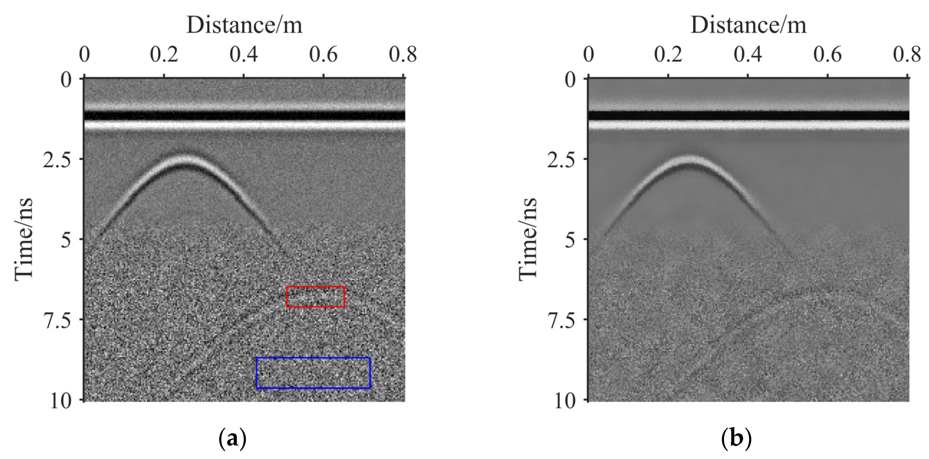
 Figure 1. The real GPR image.
 - 2
- Second, on the basis of the fourth-scale coefficient, inverse NSST is used to obtain a noise intensity distribution map, as shown in Figure 2b. In combination with Figure 1, it can be seen that the highlight coefficients at a depth of 4 ns are effective reflection signals, not noise information, and thus, this coefficient information is removed. Figure 2b shows that the real GPR image noise is not uniform, and the noise intensity varies with the time axis.
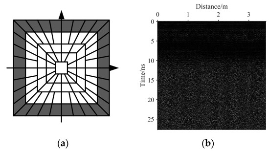 Figure 2. (a) The fourth-scale coefficient. (b) Random noise intensity distribution map.
 - 3
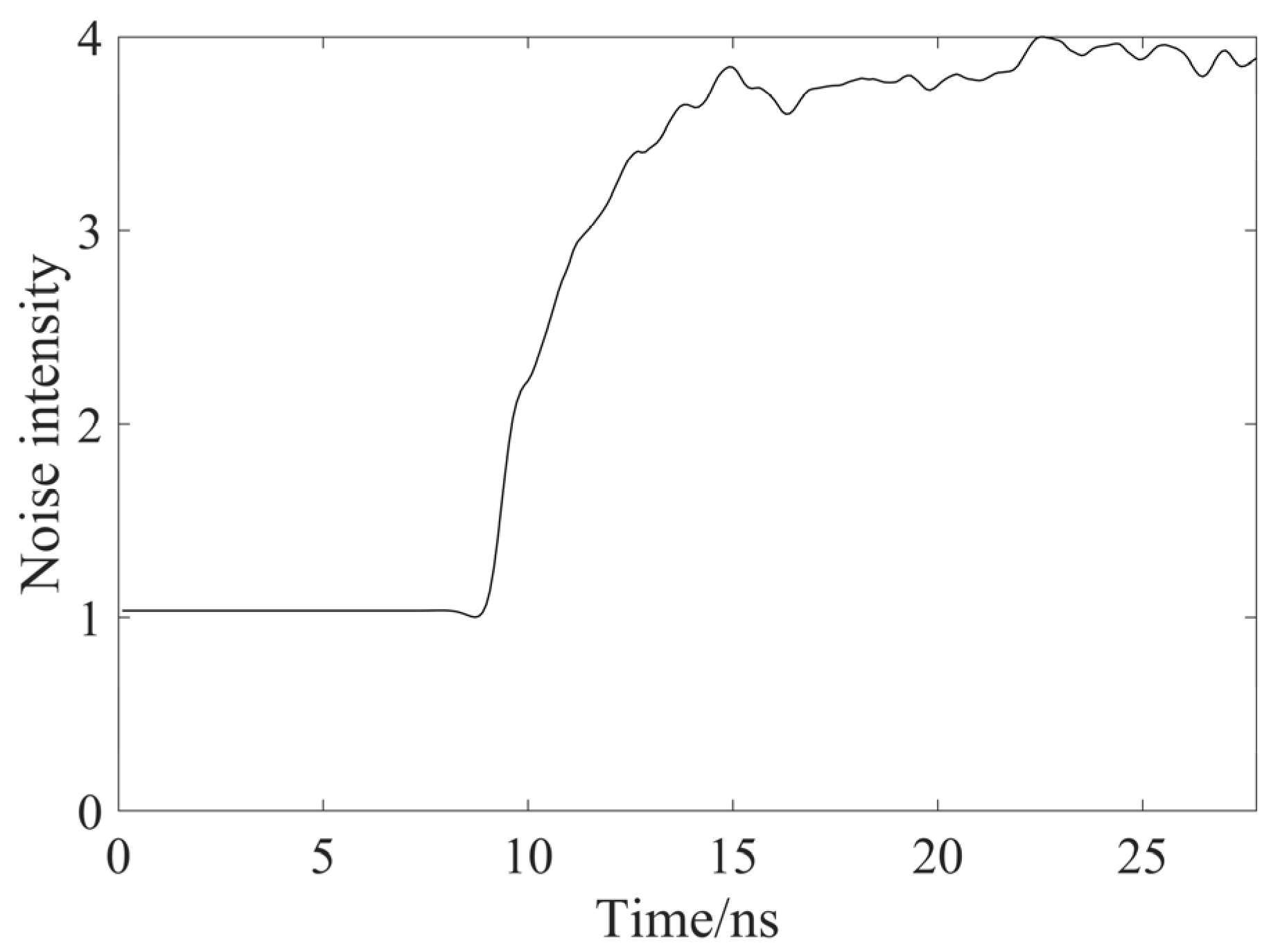
- Finally, each row of the noise intensity distribution map is summed to obtain a column vector, and the fitting function is used for the above column vector to obtain a relative noise intensity trend curve, as shown in Figure 3.
 Figure 3. Relative noise intensity trend curve.
To remove the non-uniform noise from the GPR image, a time-varying threshold function is proposed, presented as Equation (1) as follows:
where and are adjustment factors for the time-varying threshold function, with ranges of 0.1–30 and 1–3, respectively; represents the value of a noise trend curve normalised to 1–4; represents the decomposition scale of NSST; and represents the number of coefficients of NSST.
The time-varying threshold function ensures that a small threshold is used to remove shallow signal noise when the noise standard deviation is small, and a large threshold is used to remove deep signal noise when the noise standard deviation is large. Furthermore, the hard threshold shrinkage function is utilised to preserve the edge information of the image, thereby preventing the excessive smoothing of the effective information by the proposed algorithm.
2.2. Edge Area Recognition and PROTECTION
A large threshold can remove the deep signal noise with a large noise standard deviation; however, it damages the effective signal deep underground. Based on this knowledge, a method to identify and protect the edge area of GPR images is proposed. The specific steps are as follows:
- 1
- The denoised image is obtained from the result of each iteration of the proposed algorithm.
- 2
- The edge area of the denoised image is obtained using the Canny algorithm by employing the threshold .
- 3
- In the edge area, pixel differences between the noisy and denoised images are calculated. These pixel differences are adjusted using threshold . The formula for calculating the denoised image after adjustment is as follows:where is the pixel value of the denoised image after adjustment. is the pixel value of the noisy image. is the pixel difference between the noisy and denoised images before adjustment. and indicate the pixel position of the edge area.
and are adjustable parameters. Threshold is a constant, with its values in the range of 0.01–0.3. A large value of should be employed in the low-noise areas to obtain relatively more original denoising information. Moreover, a small value of should be employed in the high-noise areas to prevent the excessive smoothing of the effective information by the proposed algorithm. The formula for calculating is as follows:
where represents the trend of image noise normalised to 1–1.1. is a constant with its value in the range of 0.8–0.95.
2.3. GWO Framework for GPR Image Denoising
The performance of GPR image denoising based on NSST depends on the choice of threshold. The threshold is adjusted using the parameters and . In addition, the performance of the protection the edge area of GPR image depends on the selection of threshold and adjustment threshold . Therefore, an adequate search mechanism is needed to adjust these four parameters during each iteration of the algorithm to select the best parameter values.
In this study, NIQE is used as the cost function, and GWO is employed to select the best values for , , and . Table 1 presents the parameters of the proposed GWO framework for GPR image denoising. As shown in Figure 4, the specific steps are as follows:

Table 1.
GWO parameters.
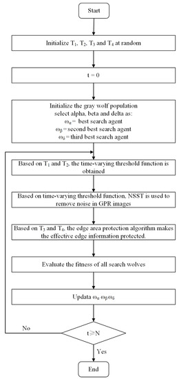
Figure 4.
Flowchart of the proposed GPR image denoising process.
- 1
- All search wolves are randomly initialised in the search space, and grey wolves α, β, and ω are selected according to the degree of fitness.
- 2
- The parameters of the grey wolves α, β, and ω are used to determine and , which are utilised to calculate the time-varying threshold function value.
- 3
- NSST is used to extract the coefficients of each frequency scale of noisy GPR images. Then, the NSST coefficients are denoised using the time-varying threshold function.
- 4
- The parameters of the grey wolves α, β, and ω are used to determine and , which are employed to protect the edge area.
- 5
- On the basis of the denoised GPR image after edge protection adjustment, the fitness of all grey wolves is evaluated. The position parameters of the grey wolves are accordingly updated.
- 6
- Determining whether the end conditions are met is necessary. If the conditions are not met, the grey wolves α, β, and ω are reselected according to the degree of fitness. Multiple iterative calculations are performed until the end conditions are met.
3. Results
A series of simulated and real GPR images are used to evaluate the denoising performance of the proposed method. A comparative denoising experiment is conducted for comparing the performances of the bilateral filter, the guided filter, NSST with different thresholds and the proposed method. The simulated GPR images are added with Gaussian noise with a noise standard deviation in the range of 10–40 to simulate the real noise environment. The range of noise standard deviation of real GPR images is 0–40. The reason for using different thresholds for NSST is that GPR image noise is non-uniform. The formula for calculating the different thresholds is presented as Equation (4). Here, the noise standard deviation is the only variable. NSST-1, NSST-2, NSST-3, and NSST-4 represent the denoising result with the noise standard deviations of 10, 20, 30, and 40, respectively.
where represents the standard deviation of noise.
Subjective and objective evaluations are made on the basis of the denoising results. The peak signal to noise ratio (PSNR) is utilised as an objective evaluation indicator for simulated GPR images. The signal-to-noise ratio (SNR) is used as an objective evaluation indicator for A-scan waveforms of different methods after denoising. The target to noise ratio (TNR) is utilised as an objective evaluation indicator for target detection performance of simulated and real GPR images and is defined as follows [30]:
where T and N represent the target and noise area, respectively—the red and blue rectangles in the original noisy GPR images; and represent the number of pixels in the target area and noise area, respectively; and represents the pixel value.
3.1. Simulated GPR Image Results
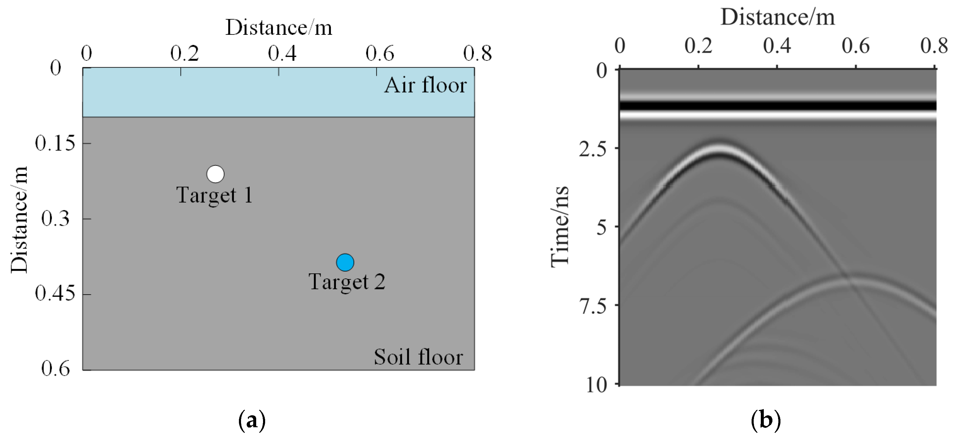
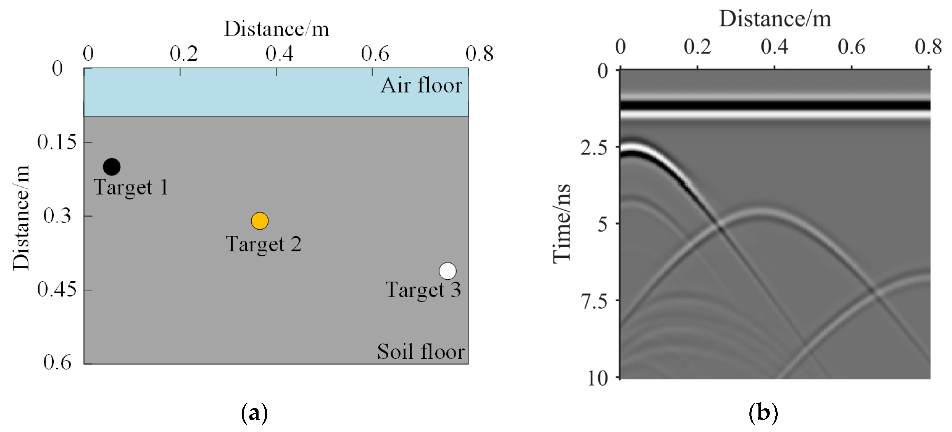
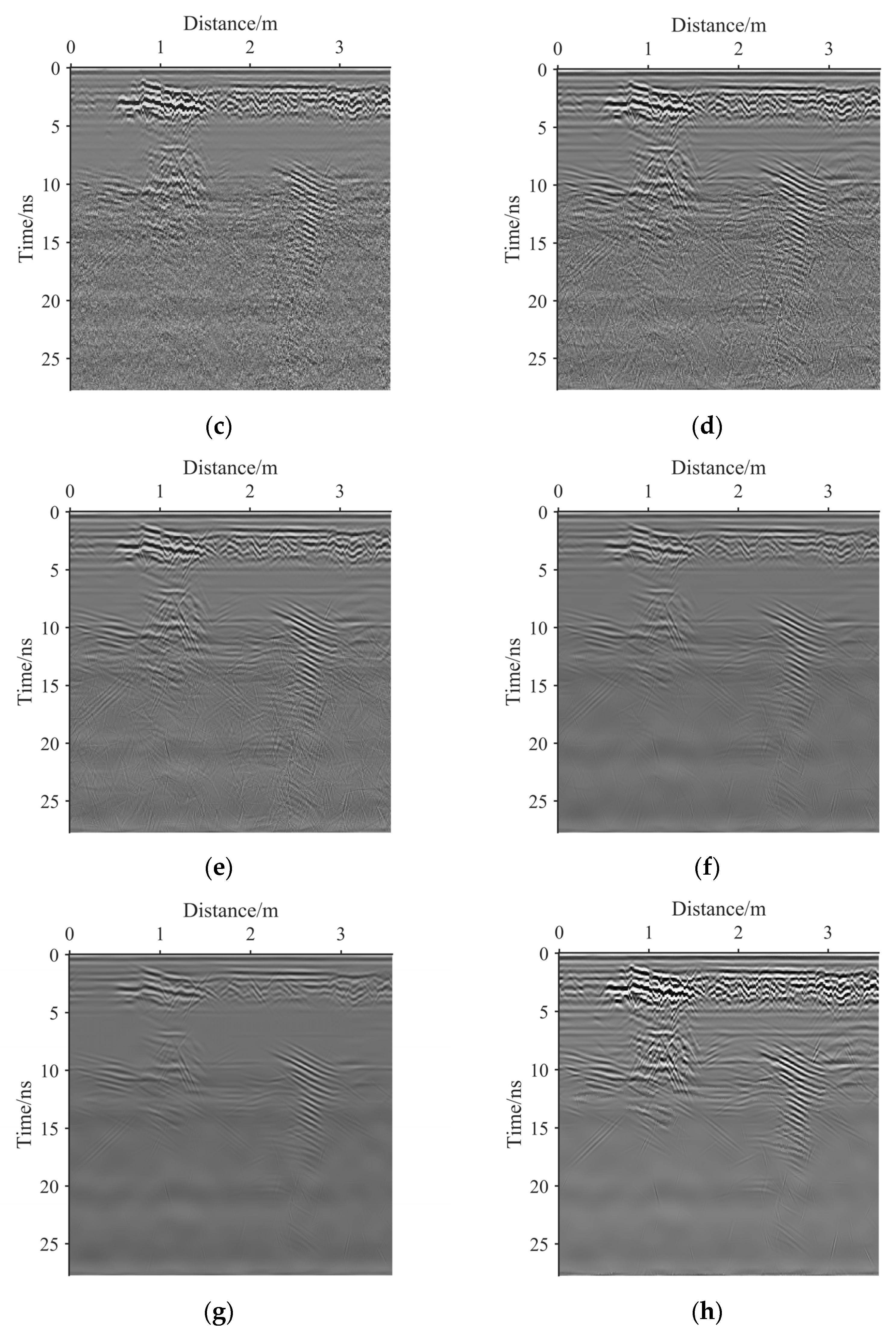
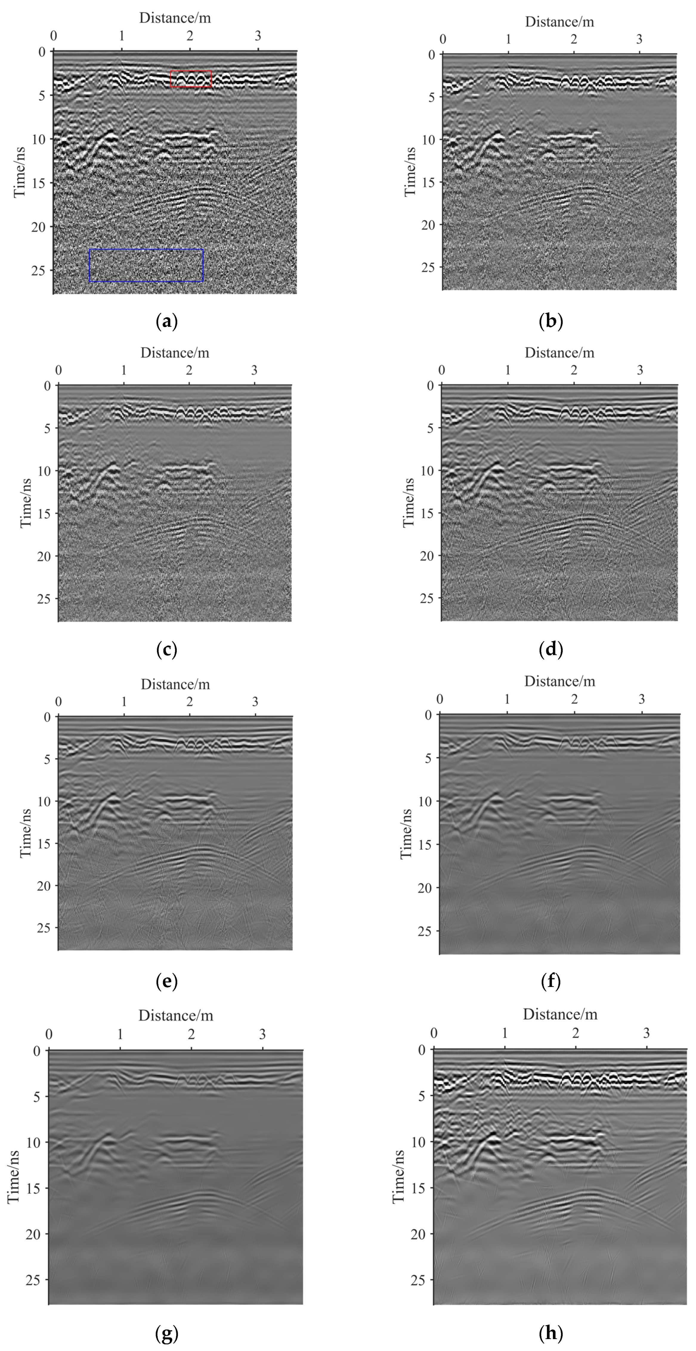
The simulated GPR images are obtained using GPRmax. A Hertzian dipole source fed with a Ricker waveform with a centre frequency of 2 GHz is used to simulate the GPR antenna. Figure 5a and Figure 6a illustrate the schematics of simulation model 1 and simulation model 2, respectively. The length of both model 1 and model 2 is 80 cm, and the depth of both models is 60 cm. The first layer of both models is air with a depth of 10 cm. The second layer of both models is soil with a relative dielectric constant of 6. Model 1 has two targets; the relative dielectric constants of targets a and b are 50 and 1, respectively, and the radius of both targets is 2 cm. Model 2 has three targets; the relative dielectric constants of targets a, b, and c are infinity, 3, and 1, respectively, and the radius of all three targets is 2 cm. The simulation data are normalised to obtain noise-free GPR images 1 and 2, as shown in Figure 5b and Figure 6b, respectively. The simulated time window is set to 10 ns. The common-offset is used. B-scan over a distance of 800 mm is obtained with a step of 2 mm.
Figure 5.
(a) GPRmax simulation model 1. (b) Simulated noise-free GPR image 1.

Figure 6.
(a) GPRmax simulation model 2. (b) Simulated noise-free GPR image 2.
To simulate the random noise in real GPR images, time-varying Gaussian noise is added to the simulated noise-free GPR images. The curve of time-varying Gaussian noise is shown in Figure 7.
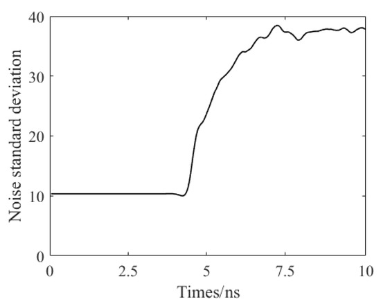
Figure 7.
Simulated noise trend curve.
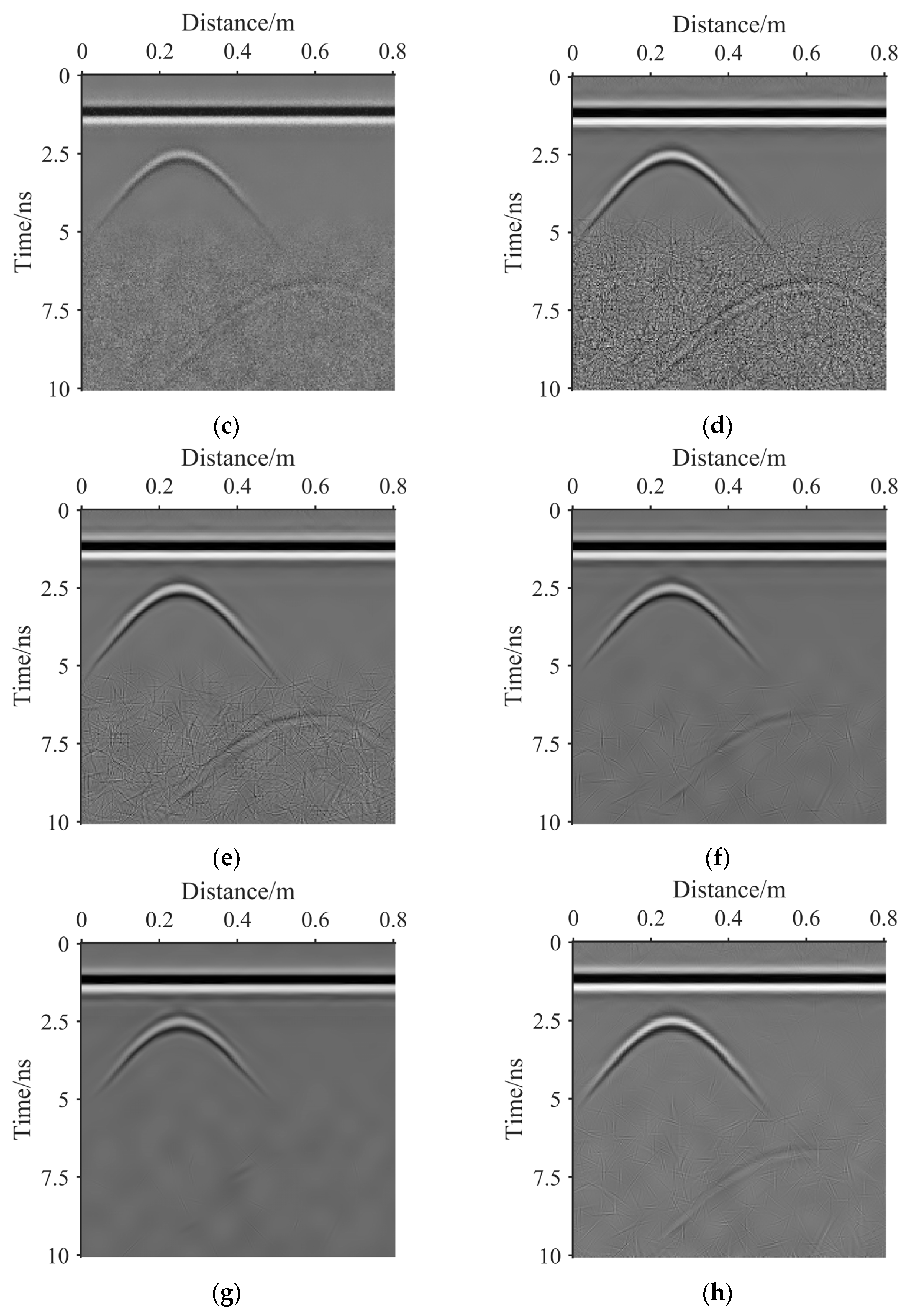
Figure 8 and Figure 9 show the denoising results of simulated GPR image 1 and image 2, respectively. From a visual perspective, the following conclusions can be drawn:
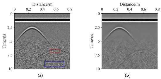
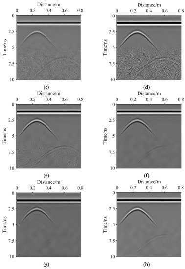
Figure 8.
(a) The simulated noisy GPR image 1. (b) The result of bilateral filter. (c) The result of guided filter. (d) The result of NSST-1. (e) The result of NSST-2. (f) The result of NSST-3. (g) The result of NSST-4. (h) The result of the proposed method.
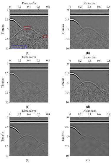
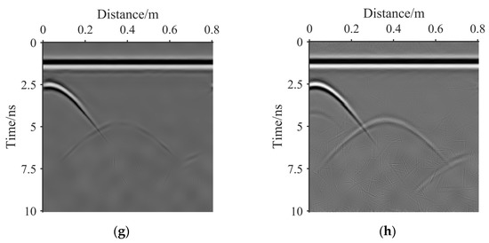
Figure 9.
(a) The simulated noisy GPR image 2. (b) The result of bilateral filter. (c) The result of guided filter. (d) The result of NSST-1. (e) The result of NSST-2. (f) The result of NSST-3. (g) The result of NSST-4. (h) The result of the proposed method.
The bilateral filter: Figure 8b and Figure 9b are the denoising results of the bilateral filter with a local window radius of 5 and a range and spatial parameters of 40, respectively. After denoising, the basic outline of the effective signal of the image is preserved. However, there is still considerable residual noise in the image.
The guided filter: Figure 8c and Figure 9c are the denoising results of the guided filter with a local window radius of 5 and the regularisation parameter of 502. The residual noise of the image after denoising is less than that denoised by the bilateral filter, and the protection of effective signal is similar to that processed by the bilateral filtering. However, after denoising, the image contrast weakens.
NSST-1: Figure 8d and Figure 9d are the denoising results of NSST with the noise standard deviation of 10. Among the denoising results of NSST-1, NSST-2, NSST-3 and NSST-4, the edge information denoised by NSST-1 at 0 ns–5 ns is best preserved. However, the residual noise denoised by NSST-1 at 5 ns–10 ns has the worst suppression effect. This is because the noise standard deviation of 10 is suitable for the noise of shallow underground; however, it is small for the noise from deep underground.
NSST-2: Figure 8e and Figure 9e are the noise removal results of the NSST with the noise standard deviation of 20. The edge information destruction at 0–5 ns is more severe than that from NSST-1. The residual noise at 5–10 ns is less than that from NSST-1. This is because the selected noise standard deviation is greater than that in the case of NSST-1. The noise standard deviation of 20 is large for shallow underground noise but small for deep underground noise.
NSST-3: Figure 8f and Figure 9f are the noise removal results of the NSST with the noise standard deviation of 30. The edge information destruction at 0–5 ns is more severe than that in the case of both NSST-1 and NSST-2. The residual noise at 5–10 ns is less than that in the case of both NSST-1 and NSST-2. This is because the selected noise standard deviation is greater than that for both NSST-1 and NSST-2. The noise standard deviation of 30 is large for shallow underground noise and small for deep underground noise.
NSST-4: Figure 8g and Figure 9g are the denoising results of NSST with the noise standard deviation of 40. Among the denoising results for the four NSST cases, the edge information denoised by NSST-4 at 0–5 ns is the most severely damaged. However, the residual noise denoised by NSST-4 at 5–10 ns is suppressed the most. This is because the noise standard deviation of 40 is suitable for the noise of deep underground; however, it is large for the noise from shallow underground.
The proposed method: Figure 8h presents the noise removal result of the proposed method with , , and of 8.96, 2.49, 0.27 and 0.85, respectively. Figure 9h shows the noise removal result of the proposed method with , , and of 7.99, 1.71, 0.10 and 0.82, respectively. At 0 ns–5 ns, the GPR image denoised using the proposed method shows the same image noise suppression and effective information protection effect as that denoised by NSST-1. At 5–10 ns, the effective information processed using the proposed algorithm is better than that processed by NSST-3 and NSST-4 but worse than that processed by NSST-1. At 5–10 ns, the residual noise processed using the proposed algorithm is less than that processed by NSST-1 and NSST-2 but more than that processed by NSST-4. Although the proposed algorithm reduces the target scattering contribution, only the proposed algorithm effectively removes the noise while retaining all the morphological characteristics of the target hyperbola. The proposed algorithm can improve the target detection performance of GPR images better than other algorithms.
Figure 10 shows the SNR results of the noise removal results for the simulated GPR images obtained using different methods. The proposed method is better than the other denoising algorithms.
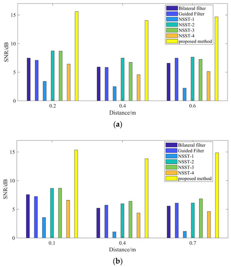
Figure 10.
(a) The SNR results of different denoising methods for the simulated noisy GPR image 1. (b) The SNR results of different denoising methods for the simulated noisy GPR image 2.
Table 2 and Table 3 present the PSNR and TNR results between the denoising results obtained using different methods and the original noise-free GPR images. The PSNR results of NSST-1, NSST-2, NSST-3 and NSST-4 show that a single denoising threshold cannot achieve perfect denoising results. The PSNR of NSST-4 is less than that of NSST-2 and NSST-3, indicating that a large threshold can suppress noise well, but it also damages the effective signal, resulting in a decrease in the final denoising effect. Hence, a single fixed threshold is not suitable for GPR image noise with non-uniformity. The proposed time-varying threshold function makes the denoising threshold conform to the trend of noise change in GPR images. Therefore, the proposed algorithm can obtain the best denoising effect. The TNR reflects the contrast between the target and noise area. Because the noisy GPR image contains considerable noise, it affects the target detection performance, resulting in a substantially low TNR value. The GPR image processed using the proposed algorithm has the largest TNR value, indicating that although the proposed algorithm has caused some damage to the original effective signal, it suppresses the noise considerably well, and finally the proposed algorithm can best improve the target detection performance of GPR images.
Table 2.
PSNR results of different denoising methods.
Table 3.
TNR results of different denoising methods.
In general, from the simulated GPR image experiment, the proposed algorithm can effectively suppress noise while protecting the effective information of the edge of the image.
3.2. Real GPR Image Results
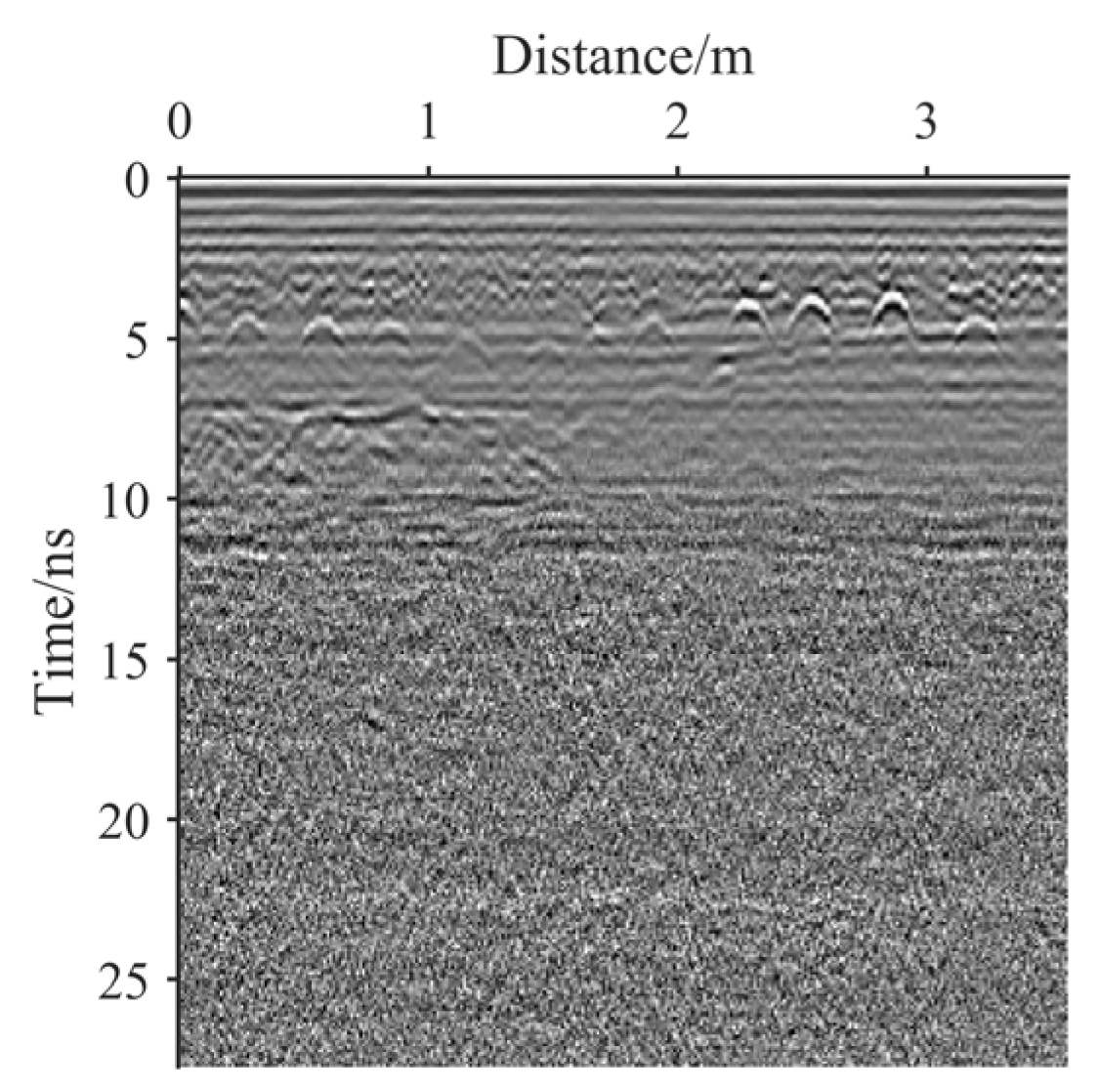
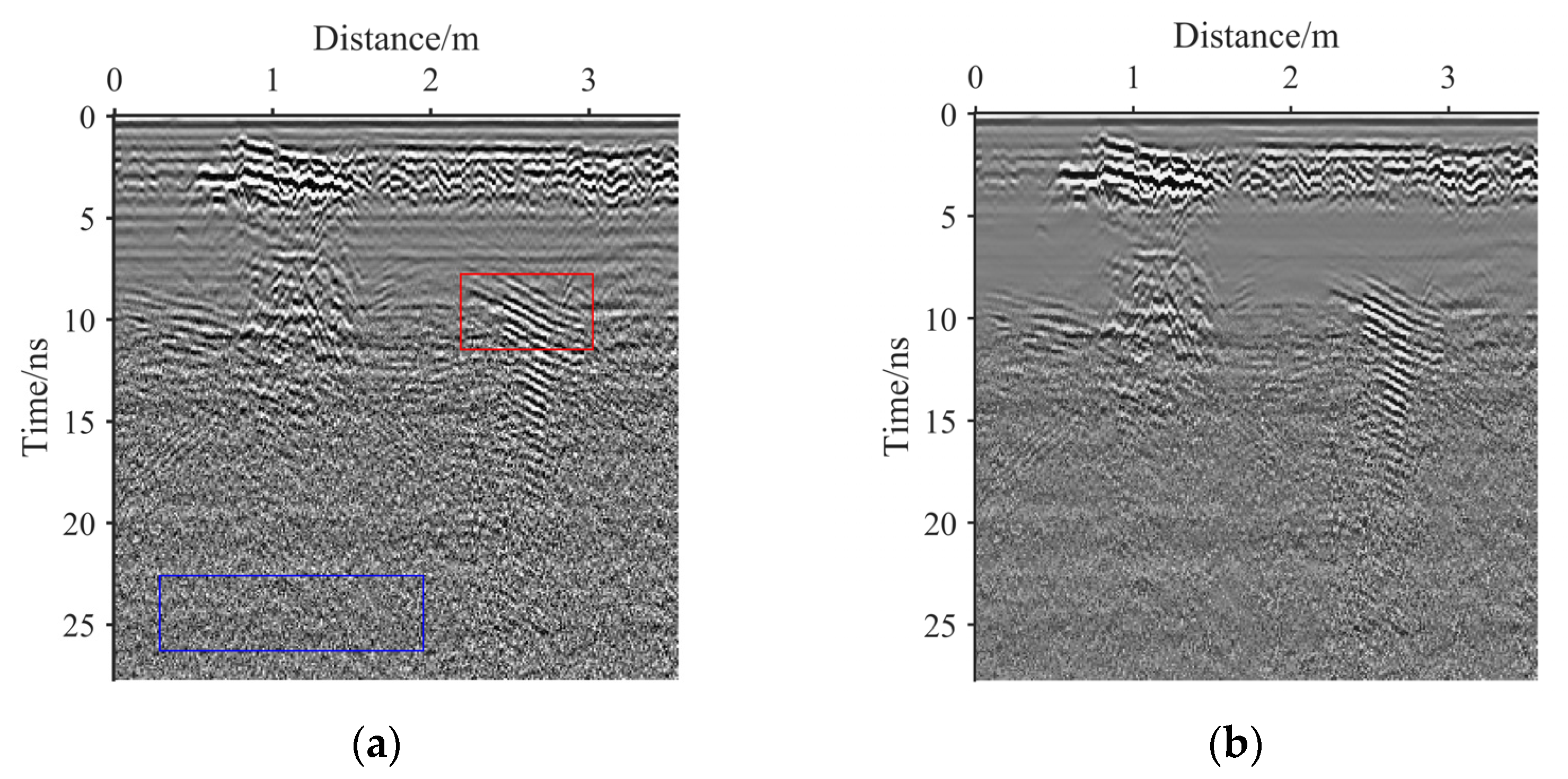
The real GPR images were obtained on the asphalt pavement of the campus of Huazhong University of Science and Technology in China by using the FastWave series of GPR produced by Ingegneria dei Sistemi. The asphalt road used for exploration is Zuiwan Road, starting at the intersection of Zuiwan Road and Nanyi Road, and ending at the intersection of Zuiwan Road and Beiyi Road. The antenna model and centre frequency are TRHF and 2 GHz, respectively. The number of sampling points is 512. The time window is 28 ns, and the spatial sampling interval is 0.01 m. The data in a total of 3000 channels of data are collected. As shown in Figure 11a and Figure 12a, the real GPR images contain effective signals and random noise. Because the noise in the real GPR image is non-uniform, the noise standard deviation of the image cannot be accurately estimated, indicating that the threshold function used by the traditional NSST denoising algorithm is not suitable for real GPR image denoising.
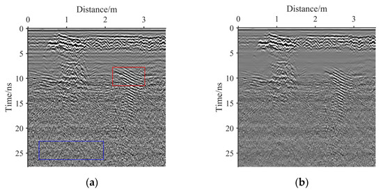

Figure 11.
(a) The original real GPR image 1. (b) The result of bilateral filter. (c) The result of guided filter. (d) The result of NSST-1. (e) The result of NSST-2. (f) The result of NSST-3. (g) The result of NSST-4. (h) The result of the proposed method.
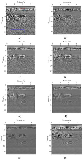
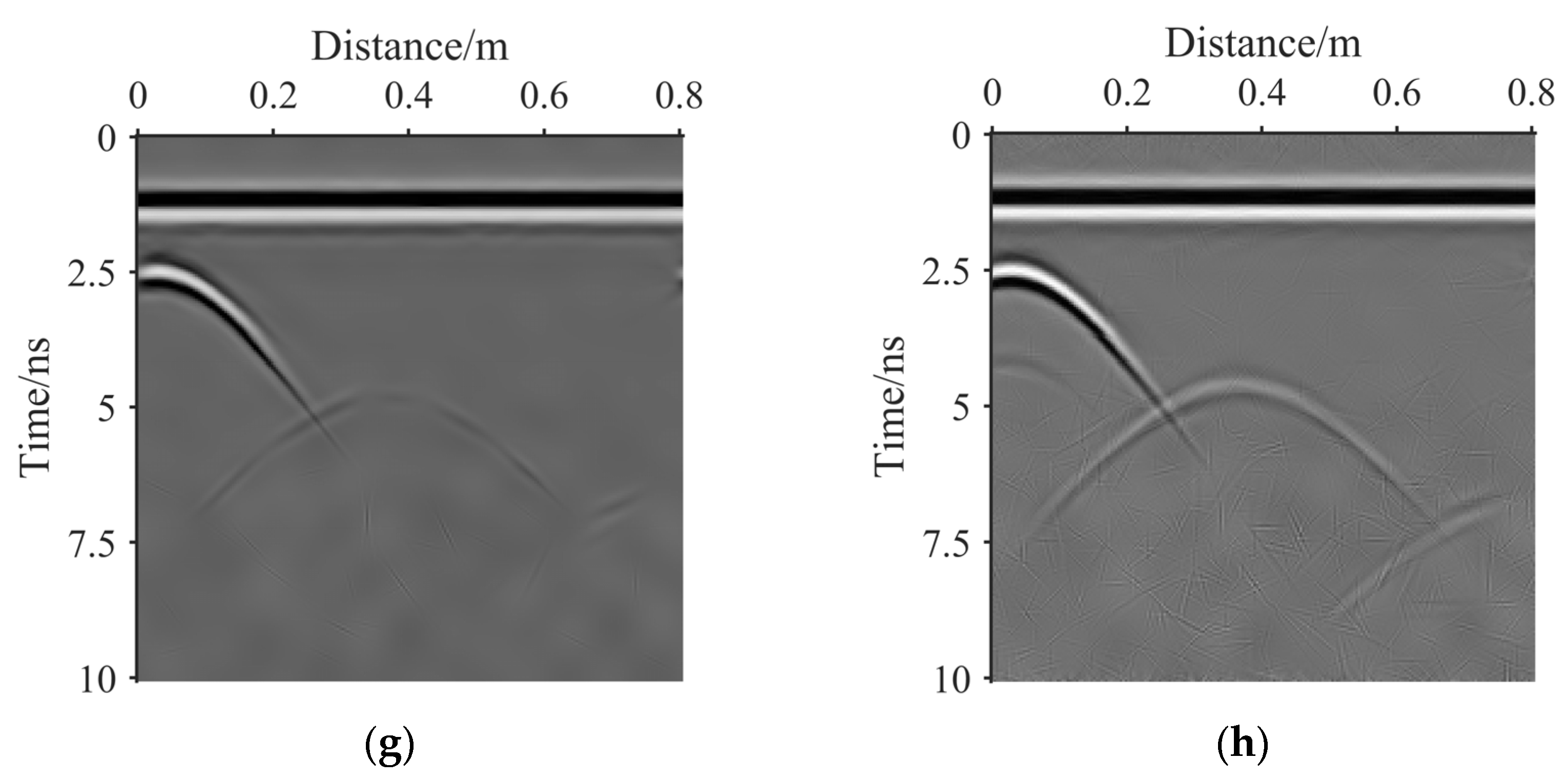
Figure 12.
(a) The original real GPR image 2. (b) The result of bilateral filter. (c) The result of guided filter. (d) The result of NSST-1. (e) The result of NSST-2. (f) The result of NSST-3. (g) The result of NSST-4. (h) The result of the proposed method.
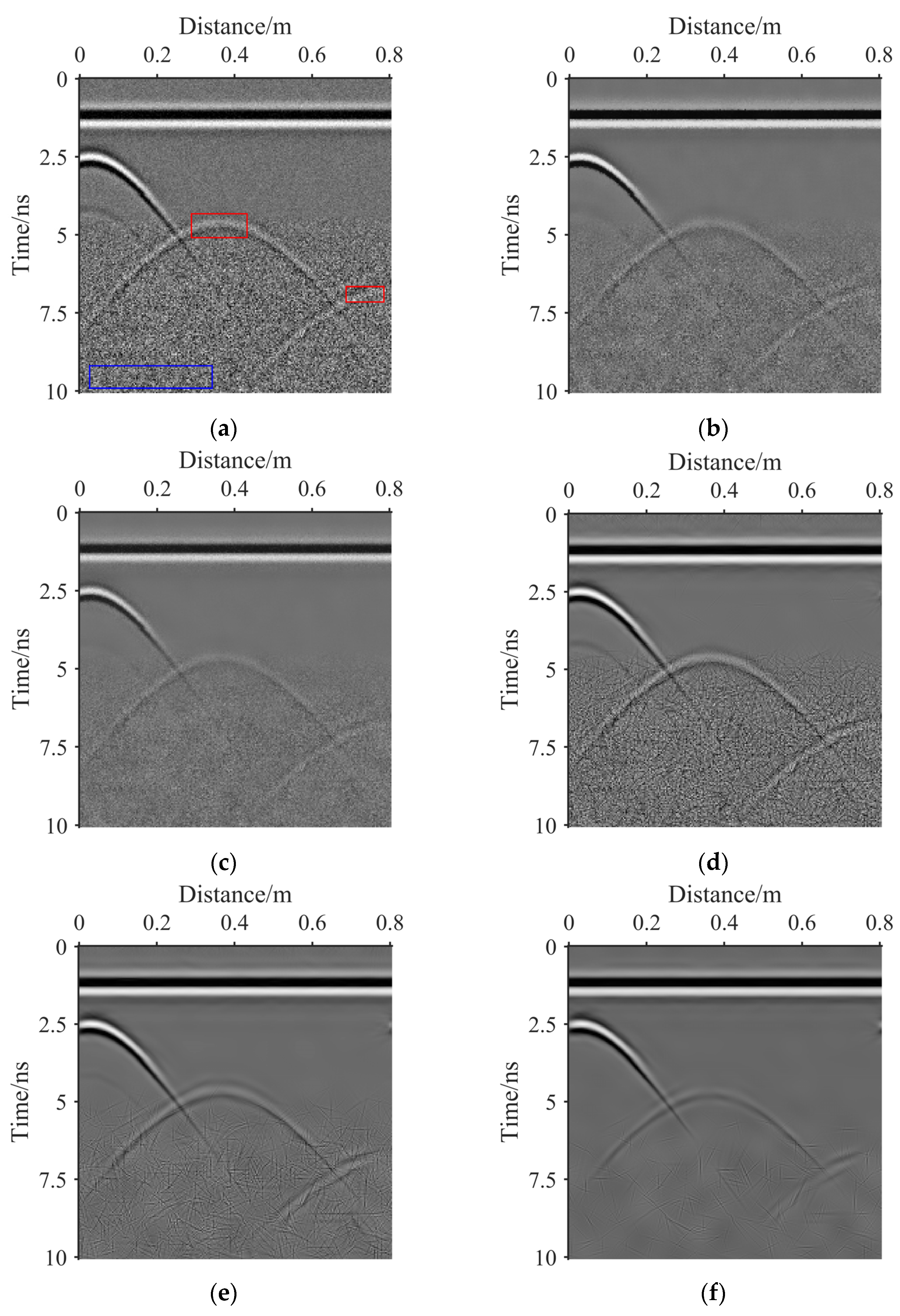
Figure 11 and Figure 12 show the noise removal results of the real GPR images 1 and 2, respectively. Visually, the following conclusions are drawn:
The bilateral filter: b and Figure 12b are the denoising results of the bilateral filter with a local window radius of 5 and a range and spatial parameters of 40, respectively. After denoising, the basic outline of the effective signal of the image is preserved. However, there is still considerable residual noise in the image.
The guided filter: c and Figure 12c are the denoising results of the guided filter with a local window radius of 5 and the regularisation parameter of 502. The residual noise of the image after denoising is less than that denoised by the bilateral filter, and the protection of effective signal is similar to that processed by the bilateral filtering. However, after denoising, the image contrast weakens.
NSST-1: d and Figure 12d show the denoising results of NSST with a noise standard deviation of 10. Among the denoising results of NSST-1, NSST-2, NSST-3, and NSST-4, the edge information denoised by NSST-1 at 0–5 ns and 10–15 ns is best preserved. However, the residual noise denoised by NSST-1 at 15–25 ns has the worst suppression effect. This is because GPR image noise is non-uniform. The noise standard deviation of 10 is suitable for the noise from shallow underground; however, it is small for the noise from deep underground.
NSST-2: e and Figure 12e show the noise removal results of NSST with a noise standard deviation of 20. The edge information destruction at 0–5 ns and 10–15 ns is more severe than that from NSST-1. The residual noise at 15–25 ns is less than that from NSST-1. This is because the selected noise standard deviation is greater than that in the case of NSST-1. The noise standard deviation of 20 is large for shallow underground noise but small for deep underground noise.
NSST-3: f and Figure 12f show the noise removal results of NSST with a noise standard deviation of 30. The edge information destruction at 0–5 ns and 10–15 ns is more severe than that in the case of both NSST-1 and NSST-2. The residual noise at 15–25 ns is less than that in the case of both NSST-1 and NSST-2. This is because the selected noise standard deviation is greater than that for both NSST-1 and NSST-2. The noise standard deviation of 30 is large for shallow underground noise and small for deep underground noise.
NSST-4: g and Figure 12g show the denoising results of NSST with a noise standard deviation of 40. Among the denoising results for the four NSST cases, the edge information denoised by NSST-4 at 0–5 ns and 10–15 ns is the most severely damaged. However, the residual noise denoised by NSST-4 at 15–25 ns is suppressed the most. This is because GPR image noise is non-uniform. The noise standard deviation of 40 is suitable for the noise from deep underground; however, it is large for the noise from shallow underground.
The proposed method: Figure 11h presents the noise removal result of the proposed method with , , and of 13.14, 1.78, 0.15 and 0.87, respectively. Figure 12h shows the noise removal result of the proposed method with , , and of 12.80, 1.77, 0.24 and 0.89, respectively. At 0–5 ns, the GPR image denoised with the proposed method shows the same image noise suppression and effective information protection effect as that denoised by NSST-1. At 15–28 ns, the effective information processed with the proposed algorithm is better than that processed by NSST-1, NSST-2, NSST-3 and NSST-4. At 15–28 ns, the residual noise processed using the proposed algorithm is less than that denoised by NSST-1, NSST-2 and NSST-3 but more than that denoised by NSST-4. Although the proposed algorithm reduces the target scattering contribution, only the proposed algorithm effectively removes the noise while retaining all the morphological characteristics of the target hyperbola. The proposed algorithm can improve the target detection performance of GPR images better than other algorithms.
Table 4 presents the TNR results of the real GPR image 1 and image 2 obtained using different methods. TNR reflects the contrast between the target and noise area. Because the real noisy GPR image contains considerable noise, it affects the target detection performance, resulting in a substantially low TNR value. The GPR image processed using the proposed algorithm has the largest TNR value, indicating that although the proposed algorithm causes some damage to the original effective signal, it suppresses the noise well. The proposed algorithm can best improve the target detection performance of GPR images.
Table 4.
TNR results of different denoising methods.
Overall, the proposed method exhibits the optimal performance in removing non-uniform noise while preserving the edge signals.
4. Discussion
As mentioned in Section 3.1 and Section 3.2, subjective and objective evaluations are used to analyse the denoising performance of the proposed algorithm. Subjective evaluation shows that although the proposed algorithm reduces the target scattering contribution, only the proposed algorithm effectively removes the noise while retaining all the morphological characteristics of the target hyperbola. Objective evaluation indicators also confirm these results. The proposed algorithm can improve the target detection performance of GPR images better than other algorithms.
By analysing and calculating the noise intensity of the real GPR image, it can be seen that the GPR noise intensity is unevenly distributed along the time axis. Therefore, the time-varying threshold function optimised using GWO has a better denoising effect on the non-uniform GPR image noise. The small threshold is used to remove the shallow signal noise when the noise standard deviation is small, and the large threshold is used to remove the deep signal noise when the noise standard deviation is large. In addition, the proposed edge area recognition and protection algorithm make the effective edge information relatively better protected.
Direct wave removal is also an important part of the research for GPR image denoising. The proposed algorithm does not provide a solution to remove the GPR direct wave. In future, we will study how to remove the direct wave effectively, while avoiding the introduction of artefacts and damage to the effective signal.
5. Conclusions
In this study, a novel GWO framework for GPR image denoising based on the NSST domain is proposed. Denoising comparison experiments suggest that the appropriate threshold is crucial for GPR image denoising. Owing to the non-uniformity of GPR image noise, the use of a single fixed threshold for noisy coefficients in each sub-band is inappropriate. Therefore, the proposed time-varying threshold function makes the denoising threshold conform to the trend of noise change in GPR images. In addition, the proposed edge area protection algorithm makes the effective edge information relatively better protected. Finally, the values of , , and are selected through GWO, which improves the performance of the time-varying threshold function and the edge protection algorithm. Thus, the proposed method provides the best noise removal results for GPR images.
Author Contributions
Methodology X.H.; software X.H.; validation X.H.; formal analysis X.L.; investigation C.W.; data curation R.Z.; writing—original draft preparation X.H.; writing—review and editing X.H.; visualisation X.H.; supervision X.L. All authors have read and agreed to the published version of the manuscript.
Funding
This research received no external funding.
Institutional Review Board Statement
Not applicable.
Informed Consent Statement
Not applicable.
Data Availability Statement
Not applicable.
Conflicts of Interest
The authors declare no conflict of interest.
References
- Utsi, E.C. Ground Penetrating Radar: Theory and Practice; Butterworth-Heinemann: Oxford, UK, 2017. [Google Scholar]
- Jol, H.M. Ground Penetrating Radar Theory and Applications; Elsevier: Amsterdam, The Netherlands, 2008. [Google Scholar]
- Diamanti, N.; Annan, A.P.; Jackson, S.R.; Klazinga, D. A GPR-Based Pavement Density Profiler: Operating Principles and Applications. Remote Sens. 2021, 13, 2613. [Google Scholar] [CrossRef]
- Gabler, M.; Uhnér, C.O.J.; Sundet, N.O.; Hinterleitner, A.; Nymoen, P.; Kristiansen, M.; Trinks, I. Archaeological Prospection in Wetlands—Experiences and Observations from Ground-Penetrating Radar Surveys in Norwegian Bogs. Remote Sens. 2021, 13, 3170. [Google Scholar] [CrossRef]
- Cui, X.; Zhang, Z.; Guo, L.; Liu, X.; Quan, Z.; Cao, X.; Chen, X. The Root-Soil Water Relationship Is Spatially Anisotropic in Shrub-Encroached Grassland in North China: Evidence from GPR Investigation. Remote Sens. 2021, 13, 1137. [Google Scholar] [CrossRef]
- Garrido, I.; Solla, M.; Lagüela, S.; Fernández, N. IRT and GPR techniques for moisture detection and characterisation in buildings. Sensors 2020, 20, 6421. [Google Scholar] [CrossRef]
- Šipoš, D.; Gleich, D. A lightweight and low-power UAV-borne ground penetrating radar design for landmine detection. Sensors 2020, 20, 2234. [Google Scholar] [CrossRef] [PubMed] [Green Version]
- Feng, D.; Liu, S.; Yang, J.; Wang, X.; Wang, X. The Noise Attenuation and Stochastic Clutter Removal of Ground Penetrating Radar Based on the K-SVD Dictionary Learning. IEEE Access 2021, 9, 74879–74890. [Google Scholar] [CrossRef]
- Bi, W.; Zhao, Y.; An, C.; Hu, S. Clutter elimination and random-noise denoising of GPR signals using an SVD method based on the Hankel matrix in the local frequency domain. Sensors 2018, 18, 3422. [Google Scholar] [CrossRef] [Green Version]
- Zhang, X.; Feng, X.; Zhang, Z.; Kang, Z.; Chai, Y.; You, Q.; Ding, L. Dip filter and random noise suppression for GPR B-scan data based on a hybrid method in f-x domain. Remote Sens. 2019, 11, 2180. [Google Scholar] [CrossRef] [Green Version]
- Xue, W.; Luo, Y.; Yang, Y.; Huang, Y. Noise suppression for gpr data based on svd of window-length-optimized hankel matrix. Sensors 2019, 19, 3807. [Google Scholar] [CrossRef] [Green Version]
- Shong, W.; Wu, H. The application of the wavelet transform technique to data processing in GPR. Geophys. Geochem. Explor. 2004, 1, 69–72. [Google Scholar]
- Baili, J.; Lahouar, S.; Hergli, M.; Amimi, A.; Besbes, K. Denoising of GPR Signals Based on the Discrete Wavelet Transform. In Proceedings of the Second International Conference on Machine Intelligence, Tozeur, Tunisia, 5–7 November 2005; pp. 103–134. [Google Scholar]
- Baili, J.; Lahouar, S.; Hergli, M.; Al-Qadi, I.L.; Besbes, K. GPR signal de-noising by discrete wavelet transform. Ndt Int. 2009, 42, 696–703. [Google Scholar] [CrossRef]
- Candès, E.J.; Donoho, D.L. New tight frames of curvelets and optimal representations of objects with piecewise C2 singularities. Commun. Pure Appl. Math. J. Courant Inst. Math. Sci. 2004, 57, 219–266. [Google Scholar] [CrossRef]
- Guo, K.; Kutyniok, G.; Labate, D. Sparse multidimensional representations using anisotropic dilation and shear operators. In Proceedings of the International Conference on the Interaction between Wavelets and Splines, Athens, Greece, 10–14 November 2006. [Google Scholar]
- Easley, G.; Labate, D.; Lim, W.-Q. Sparse directional image representations using the discrete shearlet transform. Appl. Comput. Harmon. Anal. 2008, 25, 25–46. [Google Scholar] [CrossRef] [Green Version]
- Bao, Q.-Z.; Li, Q.-C.; Chen, W.-C. GPR data noise attenuation on the curvelet transform. Appl. Geophys. 2014, 11, 301–310. [Google Scholar] [CrossRef]
- Terrasse, G.; Nicolas, J.-M.; Trouve, E.; Drouet, E. Application of the Curvelet Transform for Clutter and Noise Removal in GPR Data. IEEE J. Sel. Top. Appl. Earth Obs. Remote Sens. 2017, 10, 4280–4294. [Google Scholar] [CrossRef]
- Wang, X.; Liu, S. Noise suppressing and direct wave arrivals removal in GPR data based on Shearlet transform. Signal Process. 2017, 132, 227–242. [Google Scholar] [CrossRef]
- Wen, J.; Li, Z.; Xiao, J. Noise removal in tree radar B-scan images based on shearlet. Wood Res. 2020, 65, 1–12. [Google Scholar] [CrossRef]
- Goyal, B.; Dogra, A.; Agrawal, S.; Sohi, B.; Sharma, A. Image denoising review: From classical to state-of-the-art approaches. Inf. Fusion 2019, 55, 220–244. [Google Scholar] [CrossRef]
- Mirjalili, S.; Mirjalili, S.M.; Lewis, A. Grey wolf optimizer. Adv. Eng. Softw. 2014, 69, 46–61. [Google Scholar] [CrossRef] [Green Version]
- Zhang, Y.; Jin, Z.; Chen, Y. Hybridizing grey wolf optimization with neural network algorithm for global numerical optimization problems. Neural Comput. Appl. 2020, 32, 10451–10470. [Google Scholar] [CrossRef]
- Khairuzzaman, A.K.M.; Chaudhury, S. Multilevel thresholding using grey wolf optimizer for image segmentation. Expert Syst. Appl. 2017, 86, 64–76. [Google Scholar] [CrossRef]
- Marot, J.; Migliaccio, C.; Lantéri, J.; Lauga, P.; Bourennane, S.; Brochier, L. Joint Design of the Hardware and the Software of a Radar System with the Mixed Grey Wolf Optimizer: Application to Security Check. Remote Sens. 2020, 12, 3097. [Google Scholar] [CrossRef]
- Kennedy, J.; Eberhart, R. Particle swarm optimization. In Proceedings of the ICNN’95 International Conference on Neural Networks, Perth, Australia, 27 November–1 December 1995; Volume 4, pp. 1942–1948. [Google Scholar]
- Karaboga, D. An Idea Based on Honey Bee Swarm for Numerical Optimization; Erciyes University: Kayseri, Turkey, 2005. [Google Scholar]
- Yang, X.-S.; Deb, S. Cuckoo search via Lévy flights. In Proceedings of the 2009 World Congress on Nature & Biologically Inspired Computing (NaBIC), Coimbatore, India, 9–11 December 2009; pp. 210–214. [Google Scholar]
- Kumlu, D.; Erer, I.; Kaplan, N.H. Low complexity clutter removal in GPR images via lattice filters. Digit. Signal Process. 2020, 101, 102724. [Google Scholar] [CrossRef]


Publisher’s Note: MDPI stays neutral with regard to jurisdictional claims in published maps and institutional affiliations. |
© 2021 by the authors. Licensee MDPI, Basel, Switzerland. This article is an open access article distributed under the terms and conditions of the Creative Commons Attribution (CC BY) license (https://creativecommons.org/licenses/by/4.0/).