Electromagnetic Scattering Model for Far Wakes of Ship with Wind Waves on Sea Surface

Abstract

A comprehensive electromagnetic scattering model for ship wakes on the sea surface is proposed to study the synthetic aperture radar (SAR) imagery for ship wakes. Our model considers a coupling of various wave systems, including Kelvin wake, turbulent wake, and the ocean ambient waves induced by the local wind. The fluid–structure coupling between the ship and the water surface is considered using the Reynolds–averaged Navier–Stokes (RANS) equation, and the wave–current effect between the ship wake and wind waves is considered using the wave modulation model. The scattering model can better describe the interaction of the ship wakes on sea surface and illustrates well the features of the ship wakes with local wind waves in SAR images.

1. Introduction

Ship wakes on a random sea surface usually contain multiple wave modes and systems. Their SAR images are not the same under different conditions. The differences include the wave patterns, visibilities, brightness and darkness variations, etc. The understanding of the electromagnetic scattering mechanism of various wakes in random sea waves are of great importance in the naval ship detection, recognition and motion parameter estimation.

The earliest research on ship wakes can be traced back to Lord Kelvin in the 19th century. He found that in deep water, ship waves consisted of the transverse and divergence, two wave systems. These ship waves are distributed in a fixed angle of approximately 39°, provided that the ambient waves and currents are negligible [1]. The wake is named Kelvin wake. Since then, various ship wakes with different patterns have been reported widely. For example, some ship wakes appear narrower than the Kelvin’s angle, which is attributed to some specific ship parameters or environmental conditions, like the Froude number, water depth, wind waves and current effects, etc. [2,3,4]. The internal wave wake, which appears as multiple V-shaped stripes with small angles, is formed in the stratified seawater [5]. The narrow V wake, which is characterized by two unique bright lines in SAR images, is formed by the Bragg resonance with electromagnetic waves [6].

Apart from the V-shaped wakes, an abnormal bright or dark centerline distributed on the ship track is usually found in SAR images, called turbulent wake or centerline wake. Turbulent wake is a more complex phenomenon, which is attributed to the coupling of the ship hull, wake current, surface film and the ambient waves. The wake can be divided into near and far wake two parts. The near wake is mainly composed of a large number of breaking waves and foam distributed within a few ship lengths. The far wake often spreads for several kilometers as an area of a reduced roughness sea surface on the ship track, which associates to the short wave damping by turbulence [7].

Figure 1 shows some optical and synthetic aperture radar (SAR) images of ship wakes. In all SAR images shown in Figure 1d−h, the horizontal direction is the range direction and the vertical direction is the azimuth direction. On a complex sea surface, the most common ship wakes are the far wakes consisted of the Kelvin and turbulent wakes. However, most research on scattering model of ship wakes only considered the traditional Kelvin wake linearly superimposed on a random sea surface; and the interaction between the wake and sea surface was rarely studied. The research on electromagnetic scattering from the ship wakes on the complex sea surface is far from sufficient.

In terms of the research on electromagnetic scattering from the Kelvin wakes, Oumansour et al. [11] simulated the SAR image of the Kelvin wake using the two-scale method (TSM). Hennings et al. [12] compared their simulated SAR images with the measured images by the SEASAT radar to discuss the visibility of the Kelvin arms at different azimuth angles. Shemer et al. [13] proposed an interferometric SAR model for the Kelvin wakes. Arnold-Bos et al. [14] proposed a bistatic SAR imaging model for the Kelvin wakes. Zilman et al. [15] simulated lots of SAR images of Kelvin wakes under various sea conditions and electromagnetic parameters, and used the discrete Radon transform to detect the simulated Kelvin wake. The above studies have only considered the classical Kelvin wakes with linearly superimposed wind waves, the small-scale roughness variations caused by the interaction between ship wake and ambient waves were ignored.

Compared with the studies on Kelvin wakes, there are fewer electromagnetic scattering or imaging studies on turbulent wakes; because the turbulent wake, which usually appears as a flat area embedded in a complex ocean, cannot be represented by the traditional linear superposition wake model. Peltzer et al. [16] measured and studied the effects of the surfactants in turbulent wakes. Marmorino and Trump [17] completed the acoustic Doppler measurements of turbulent wakes. They found that wake appeared clearly as a band of elevated acoustic backscatter, and the horizontal currents of the turbulent wake directed outward from the wake centerline. Ermakov and Kapustin [18] studied the time dynamics of a turbulent region by the acoustic observations, and they proposed a qualitative model to describe the initial wake expansion. George and Tatnall et al. [19] simulated the SAR image of an asymmetric turbulent wake generated by a hemisphere based on its velocity field. Soloviev et al. [20] measured the ship far wake by sonar, and compared the results with the corresponding TerreSAR-X images. They found that the asymmetry of the ship far wakes were caused by the wind field on sea surface. Afterwards, Fujimura et al. [21,22] simulated the SAR image of the turbulent far wake under a cross wind field using CFD technology. The above studies all used relatively small discrete units to characterize the irregular shedding vortices from the ship. Limited to computing resources, the simulation scene is relatively small. And the effects of the realistic ambient waves were ignored. Wang et al. [23,24,25,26] conducted several electromagnetic scattering or SAR imaging studies on different types of ship wake, including the near-field breaking ship waves [23], linearly superimposed Kelvin wakes [24], narrow Kelvin wakes and the internal wave wake [25,26]. However, these models all have difficulty representing the features of various ship wakes in multi-scales.

In the former works, the different components of the wake were often studied separately, and the research on electromagnetic model for turbulent wakes are still insufficient. In order to improve our understanding of the electromagnetic scattering mechanism of ship wakes, the aim of the current investigation is to propose a more general model for the electromagnetic scattering from a ship far wake, consisting of both Kelvin wake and turbulent wake. The research can help to improve our understanding of remote sensing images for ship wakes, and to further explore more effective strategies and conditions for ship wakes observing. The proposed model evaluated the influence of sea ambient waves better by the action spectrum equilibrium equation. The wake induced by the ship was carried out by solving the Reynolds averaged Navier–Stokes (RANS) model numerically, which could obtain the entire flow field information generated by a ship. The ambient waves were considered as random wind waves. Waves of similar discrete size in ship wakes were superimposed on them, and the interaction between the wakes and ambient waves was described by the wave modulation theory [27,28]. The source terms for wind waves and turbulent wake were introduced to simulate the wave evolution in ship wake. In combination with the modulation model of the wave action spectrum, we improved our slope deterministic scattering facet model [26,29] so that it could further consider the regional changes of the wave spectrum caused by the wave–current effect. The improved model can better calculate the scattering distribution of the mixed waves by considering both the influence of large-scale slope and small-scale roughness variations on discrete facets.

2. Method

This section mainly covers three main issues for the scattering model of the ship wakes: the fluid–solid interaction between the ship and water surface, the wave–current interaction between the wake and sea waves, and the electromagnetic scattering from the sea surface. The key components of the model are mainly described in the Section 2.2, which introduced implementation of the modulation wave model to improve the traditional scattering model.

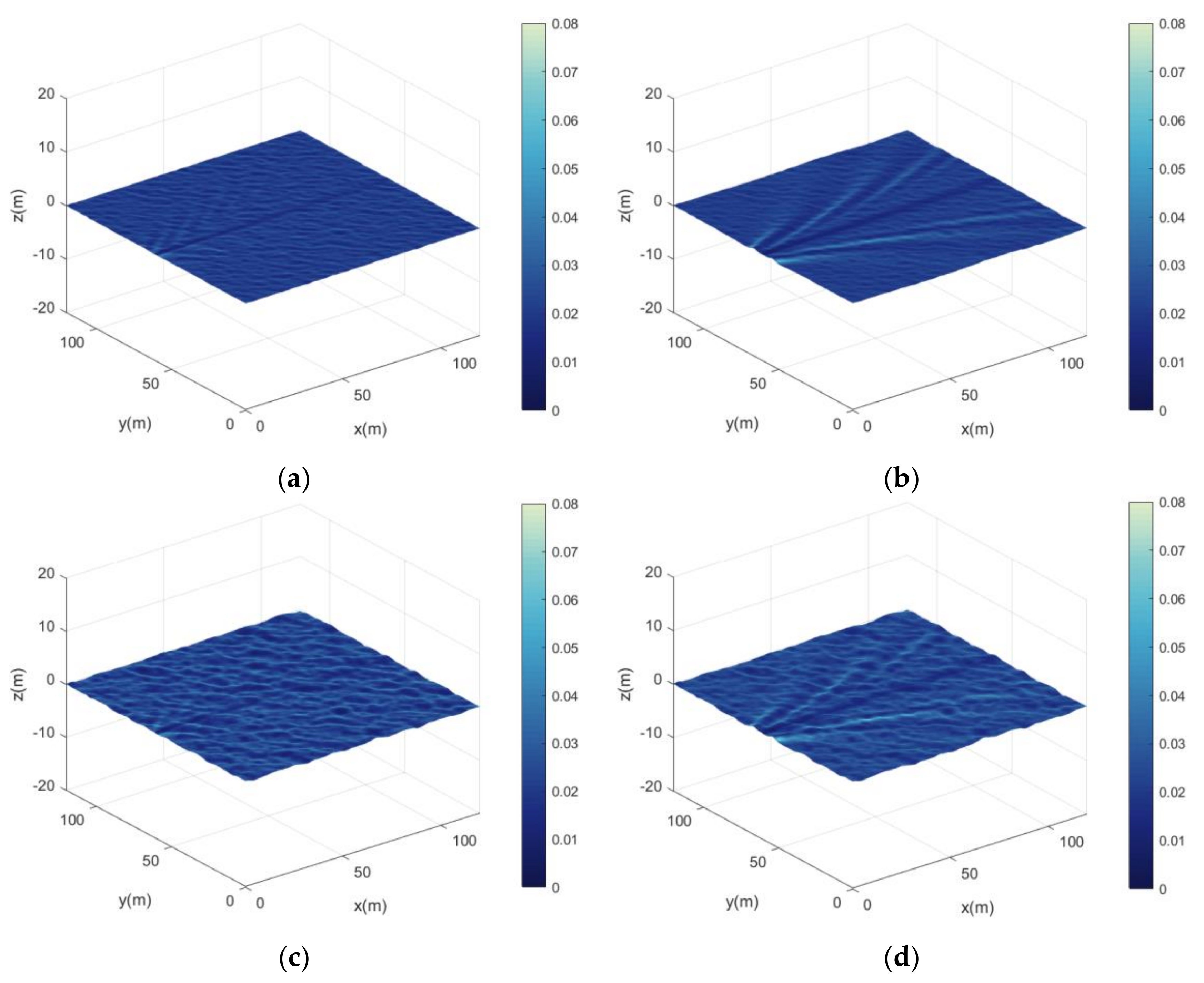
2.1. Simulation of the Ship Wake Model

In this investigation, a full three-dimensional wave model with turbulence based on the finite volume (VOF) method was used to obtain the ship wakes. The RANS equation was solved numerically and the Menter’s shear stress transport (SST) turbulence model [30] was implemented solving the general viscous and turbulent flow in the wakes. With the inclusion of the turbulence model, it is possible to simulate almost all ship wakes problems, e.g., gravity waves, breaking waves, wave–body interactions and air entrainment on the water surface.

The simulation scene for the ship wake model was from –20 m to 160 m in the x-direction and from –60 m to 60 m in the y-direction. The resolution of the far wake was 0.6 m in the horizontal direction and 0.03 m in the vertical direction, and the modeling grid consisted of about 5.94 million hexahedral cells. A bare ship hull moving at a constant speed in the negative x-direction was considered. The wakes at different ship speeds can be obtained by changing the velocity of the inlet flow. The bow of the hull was set at the origin and the hull had a length of 21.54 m, a beam of 2.88 m and a draft of 0.9 m. Other settings and schemes were consistent with our previous work [23] and would not be reiterated here.

Figure 2a–c show the elevation, the velocity in x and y direction of the resulting ship wake with the speed of 5 m/s, respectively. The characteristics of the Kelvin wake can be directly observed from the wave elevation, whereas the turbulent wake is mainly related to the velocity field. Then, we only considered the EM scattering from the far-field wake. The wake region from x = 30 m to x = 150 m illustrated in Figure 2 was extracted for the subsequent simulations, and it was reasonable to ignore the multiple scattering effects of the wave breaking and foam layers in the near ship wakes.

2.2. Modulation Spectrum Model of the Mixed Water Waves

The wave spectral model is applied to the simulation of the ambient sea waves, which is constructed on the assumption that the waves are composed of an infinite number of linear waves with random phases. The sea surface can be represented by:

$$z={\displaystyle \sum _{i=1}^{\infty }{\displaystyle \sum _{j=1}^{\infty }\sqrt{2F}\cos [k_{i}x\cos {\theta }_j+k_{j}y\sin {\theta }_j-{\omega }_{i}t+{\psi }_{ij}]}},$$

(1)

where $k_i$, ${\omega }_i$, ${\theta }_j$, and ${\psi }_{ij}$ denote the wave number, radian frequency, direction angle and initial phase, respectively. $F$ is the surface elevation variance density spectrum, which also called wave energy density function or wave spectrum. The elevations of the ship wakes were superimposed on the ambient waves; then, the interaction between the wakes and ambient waves was described by the wave modulation theory.

In a deep-water assumption, the hydrodynamic modulation effect of the surface current field can be modeled using the following action spectrum equilibrium equation [28]:

$$\frac{\partial N}{\partial t}+{\nabla }_x\cdot \dot{x}N+\frac{\partial }{\partial k}\dot{k}N+\frac{\partial }{\partial \theta }\dot{\theta }N=S/{\omega }_0,$$

(2)

$$\dot{x}=\frac{\partial x}{\partial t}=\frac{\partial \omega }{\partial k},$$

(3)

$$\dot{k}=\frac{\partial k}{\partial t}=-k\cdot \frac{\partial U}{\partial s},$$

(4)

$$\dot{\theta }=\frac{\partial \theta }{\partial t}=-\widehat{k}\cdot \frac{\partial U}{\partial m},$$

(5)

where N is the action spectral density, S is the source term. x = (x, y) is the two-dimensional spatial position. s is a coordinate in the direction θ and m is the coordinate perpendicular to s.

The relationship between the action spectral density N and the wave spectrum F of the sea surface is given by:

$$N(x,k,\theta )=\frac{F(x,k,\theta )}{{\omega }_0(k)},$$

(6)

where ${\omega }_0$ is the intrinsic angular frequency, and can be calculated as:

$${\omega }_0=\sqrt{gk+\xi {\rho }^{-1}{k}^3},$$

(7)

$\xi ={0.07\mathrm{kg}/\mathrm{s}}^2$ is the surface tension coefficient. Then, the Doppler shifted angular frequency of the current with the horizontal speed $U$ can be expressed as:

$$\omega ={\omega }_0+k\cdot U$$

(8)

The source term S represents the energy flux induced by diverse processes of the ocean waves’ motion. The source terms used to describing different problems are various. For the estimation of the electromagnetic scattering from sea surface containing ship wakes in this paper, we only considered a simplified situation with a source term S_w for the wind waves and a damping source term S_t for the impact of turbulent wakes on sea surface. The non-linear source terms S_nl for wind waves are ignored to save computational time and memory. The wind source term can be simplified into a wind wave energy input $S_{in}$ and a local wave energy dissipation $S_{ds}$:

$$S_w=S_{in}+S_{ds},$$

(9)

where $S_{in}$ can be expressed as [28]:

$$S_{in}(k,\theta )=\frac{{\rho }_a}{{\rho }_w}{\omega }_0(k)\gamma (k,\theta )F(k,\theta ),$$

(10)

$$\gamma (k,\theta )={\alpha }_{in}{G}_{in}(k,\theta )\sqrt{B_n(k)}{W}^2(k,\theta ),$$

(11)

$$W(k,\theta )=U_{10}\cos (\theta -{\phi }_w)k/{\omega }_0,$$

(12)

${\rho }_a$ and ${\rho }_w$ are the density of air and water, respectively. $U_{10}$ is the wind speed at 10 m above the sea surface. $B_n(k)=A(k)F(k)k^3$ is the normalizing of the curvature spectrum in respect to the propagation direction function, where:

$$A(k)=1/{\displaystyle {\int }_0^{2\pi }F(k,\theta )/F_{\max }(k)d\theta },$$

(13)

$W(k,\theta )$ is the wind drive parameter and ${\alpha }_{in}$ denotes the growth parameter of the sea surface, used to adjust the wind intensity of the negative input.

$${\alpha }_{in}=\left\{\begin{array}{ll}1& W(k,\theta )\ge 0\\ -0.09& W(k,\theta ) < 0 \end{array}\right..$$

(14)

The dissipation term $S_{ds}$ can be expressed as:

$$S_{ds}(k,\theta )=T(k,\theta )F(k,\theta ),$$

(15)

$$T(k,\theta )=-af{(\frac{F-F_T}{F_T})}^4,$$

(16)

where the coefficient $a=4.75\mathrm{E}-6$. $F_T={0.035}^2/k^3$ is the threshold of spectral density.

The damping source term S_t only works in the areas of turbulent wake, and is considered as [31]:

$$S_t(x,k)=\frac{-0.0015{\gamma }_t{U}_s{k}^{2/3}}{{\left(d/L_s+0.07\right)}^{4/5}{l}^{1/3}}\left[1-{\left(\frac{y}{W_t\left(x\right)}\right)}^2\right]F(k,\theta )$$

(17)

where ${\gamma }_t$ denotes the area ratio of the turbulent wake in a facet. $U_s$,$L_s$ are the ship speed and length, respectively. d is the distance from the wake to the stern. l is the integral length scale of the turbulence, and $W_t\left(x\right)$ is the width of the turbulent wake.

The initial ambient waves are regarded as a fully developed sea. The Elfouhaily directional gravity–capillary wave spectrum [32] is implemented as the initial wave spectrum in the simulations. Figure 3 gives out the wave spectrum and the corresponding normalized source terms, where ${\phi }_w$ represents the wind direction, and $k_p$ is the spatial frequency of the maximum of the spectrum.

As demonstrated in Figure 3, the wind input mainly occurs in the high-frequency region corresponding to the capillary waves, and the dissipation mainly occurs in the peak region of the sea spectrum. The source term for the turbulent wake is related to frequency and location, and mainly occurs in the high-frequency region. The wave damping of the turbulent wake is significantly stronger in the high-frequency capillary waves than in the low-frequency gravity waves.

The governing equation (2) was solved using a fractional step method which considers spatial propagation, intra-spectral propagation and source terms separately. The upstream non-oscillatory (UNO) advection scheme [33] was applied to the discretion of the spatial and spectral domain. The boundary conditions for x and k were regarded as zero gradients; and periodic boundary condition was applied for the direction angle θ. The general source term was considered as the local wind waves and current interactions. More details about the numerical approaches can be found in [28].

To illustrate the effect of the current modulation and the source term in different scales more clearly, a simple one-dimensional case is given in Figure 4. The random sea surface with the wind speed of 3 m/s was modulated by a cosine form current. The black arrows in the in the lower part of each Figure indicate the changing water currents, in which the left half is a convergent area, and the right half is a divergent area. The effect turbulent wake was not considered here. The original sample interval is 0.04 m as shown in Figure 4a, and the same results with a coarser sampling interval of 1 m are shown in Figure 4b.

Since the phases of the waves in Figure 4 come from the same random numbers, the shape of the modulated waves are closed to original waves. As shown in in Figure 4a, when the source term is set to 0, only the current modulation is considered. The wave action spectrum is equilibrium, and the wave energy will continue to transfer to the convergent area from the divergent area. The modulated sea surface becomes rougher in the left half and smoother in the right half. However, due to a lack of the constraint, the sea surface amplitude will be over modulated to an unsustainable height. The source term, especially the dissipation source, can limit these over modulations. Moreover, since the modulation function mainly works in the high frequency region of water waves, the results in Figure 4b with a coarser sampling interval cannot characterize the modulation results reasonably. Therefore, in order to characterize the ship far wakes in a large-scale two-dimensional scene, the spatially varying wave spectrum should be further considered to complete the wake modulation effect on the scales of the capillary gravity and capillary waves.

2.3. Modulation Facet Scattering Model

Based on the modulated spectrum, we improved a facet scattering model [29], which was efficient on computing the complex reflective function of a large-scope surface with high accuracy. We used the spatially varying modulated spectrum instead of a fixed statistical spectrum function so that the roughness variations of the waves could be further considered. It was noticed that the model was proposed for the bistatic scattering calculations, in which the incident waves and the scattering waves are in different directions; and the model can also complete a calculation of a backscattering case by setting equal incident and scattering directions. We only consider the case of backscattering in the simulations, because this paper mainly focuses to the ship wakes in monostation SAR images.

The contribution of the scattering field was divided into small facets, the size of which could be several times the incident wavelength. The scattering coefficient, the normalized radar backscattering cross–section (NRCS), of a single facet can be simply described by:

$${\sigma }_{PQ}^{}({\widehat{k}}_i,{\widehat{k}}_s)={\sigma }_{PQ}^{KAM}({\widehat{k}}_i,{\widehat{k}}_s)+{\sigma }_{PQ}^{TSPM}({\widehat{k}}_i,{\widehat{k}}_s),$$

(18)

where ${\widehat{k}}_i$ and ${\widehat{k}}_s$ are the unit vectors of the incident and scattering electromagnetic waves, respectively. ${\sigma }_{PQ}^{}({\widehat{k}}_i,{\widehat{k}}_s)$ is the total NRCS of the facet. The footmark PQ represents the polarization mode. ${\sigma }_{PQ}^{TSPM}({\widehat{k}}_i,{\widehat{k}}_s)$ is the Bragg resonant component of the surface and can be calculated by:

$${\sigma }_{PQ}^{TSPM}({\widehat{k}}_i,{\widehat{k}}_s)=\pi k^4{\left|\epsilon -1\right|}^2{\left|{\tilde{\mathbb{F}}}_{PQ}\right|}^2[F\left(x,q_l\right)+F\left(x,-q_l\right)]/2, \left|q_l\right|<k_{cut},$$

(19)

where $q_l$ is the projection vector of $q$ on the local xoy plane, and

$$q=k({\widehat{k}}_s-{\widehat{k}}_i),$$

(20)

$$q_l=q\cdot ({\widehat{k}}_i\times {\widehat{k}}_s),$$

(21)

$k_{cut}$ is the cutoff wavenumber, which is the diving between the large and small scale; and we regarded the $k_{cut}$ as one-third of the incident wavelength in this paper. $\epsilon$, which is the complex permittivity of seawater, can be estimated at any frequency within the microwave band using the Debye expression. Here, $\left|{\tilde{\mathbb{F}}}_{PQ}\right|$ is the polarization factor in global coordinates [24,29].

$${\sigma }_{PQ}^{KAM}({\widehat{k}}_i,{\widehat{k}}_s)=\frac{\pi k^2{\left|q\right|}^2}{q_Z^4}{\left|{\tilde{\mathbb{F}}}_{PQ}^{KAM}\right|}^{2}P(n),$$

(22)

where $\left|{\tilde{\mathbb{F}}}_{PQ}^{KAM}\right|$ is the polarization factor of the Kirchhoff approximation method (KAM) [34]; $z_x,z_y$ are the slope of the facet in x and y direction, respectively. $P(\cdot )$ represents the probability distribution of the wave slopes, which is calculated using the modulated spectrum [34]:

$$P(z_x,z_y)=\frac{F_p(z_x,z_y)}{2\pi ms{s}_{u}ms{s}_c}\exp (-\frac{z_x^2}{2ms{s}_u^2}-\frac{z_y^2}{2ms{s}_c^2}),$$

(23)

where $ms{s}_u$ and $ms{s}_c$ denote, respectively, the upwind and crosswind mean square slope (MSS) of the sea surface.

In order to validate the accuracy of the proposed method on sea surface electromagnetic estimation, we calculated the total backscattering coefficients from the sea surfaces with and without ship wake, respectively, as the verification cases. The results were compared with the experimental results in the SASS model [35]. The frequency of the electromagnetic wave is set at 14.9 GHz and the wind speeds are 5 m/s and 10 m/s, respectively.

As shown in Figure 5, the results for both HH and VV polarizations of the two models are in good agreement with the measurement results. Although the total backscattering coefficients are different slightly when the ship wakes was taken into account, the existence of the wake has a negligible effect on the total scattering from the sea surface. It is almost impossible to distinguish the contribution of the ship wake from the total scattering field of the sea surface. Therefore, it is necessary to further discuss the results of spatial distribution for the ship wakes to explore the effects of ship wakes on electromagnetic scattering.

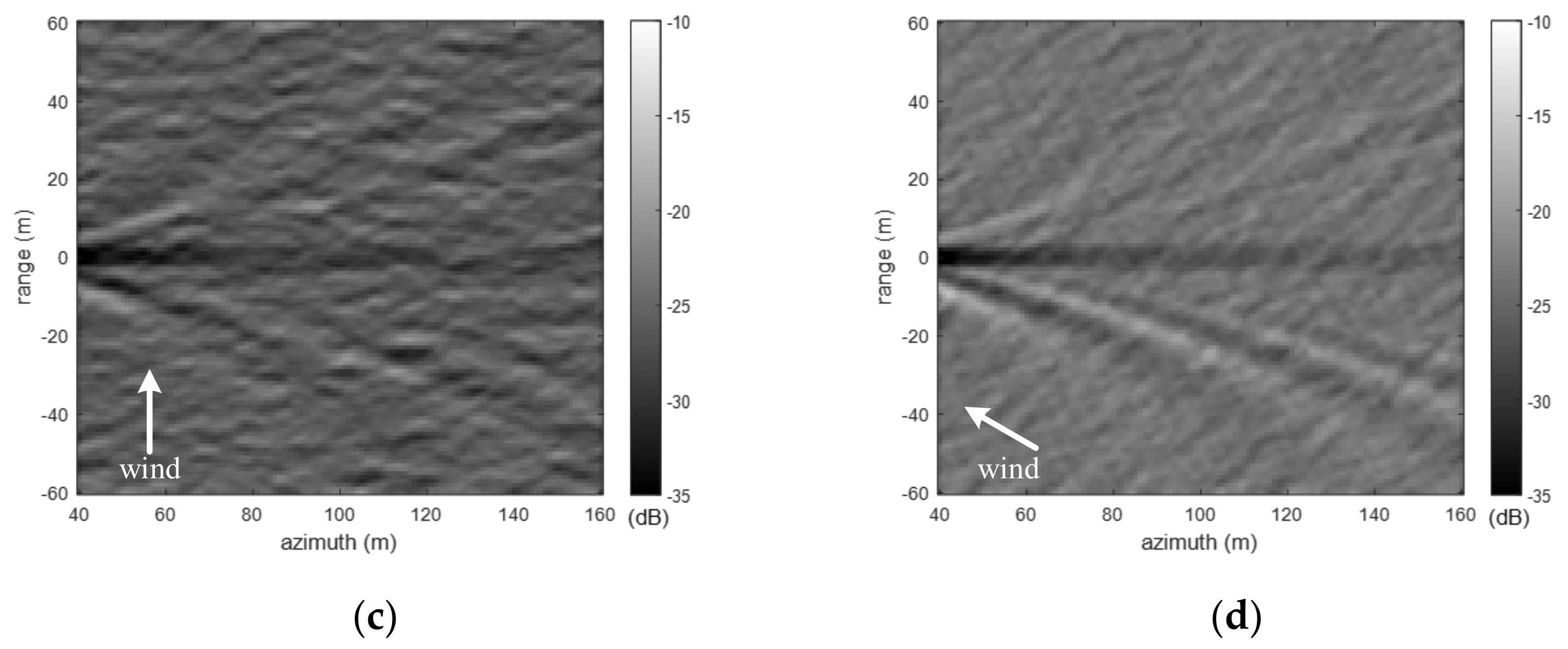
3. Simulation Results and Analysis

Figure 6a–d show the simulation results of the modulated mixed waves. The size of the simulated composite sea surface, which contains the ship far wakes embedded in random wind waves, is 120 m × 120 m; and the size of the discrete facet is 1 m × 1 m. Considering the difference between the discrete scale for the mixed wave geometry and the scale of roughness which need to be characterized, the 3D mixed waves of the ship wakes and wind waves are colored by the MSS of local waves. The ship speeds were set as 5 m/s and 10 m/s, respectively. The winds were set in the 45° direction with the speed of 3 m/s and 5 m/s, respectively.

As shown in Figure 6, since the MSS distribution of the composite sea surface can display the surface roughness variations which are much smaller than the discrete scale, the figures are consistent with the real images for a ship wake. The turbulent wake appears as a dark centerline, and the Kelvin wake appear on both sides. As the wind speed increases, the wakes are more affected by the ambient waves. Moreover, the waves of ship wake are more likely to be covered by the ambient waves when they travel in the same direction as shown in Figure 6a.

Then, based on the backscattering distributions of the modulation waves, we used the velocity bunching model to simulate the monostatic SAR images of the ship wakes on the sea surface [26]. First, we set the SAR platform moving in the y and x directions, respectively. The incident direction was set as 45°. The frequency of the electromagnetic waves was set at 9.8 GHz (X-band), HH polarization for a general airborne radar.

The electromagnetic scattering mechanism on the sea surface was dominated by the Bragg resonance effect under such conditions. The corresponding SAR images of the modulation waves with different ship and wind speeds are illustrated in Figure 7. The wind directions are indicated by white arrows in the figures. The wave component on the sea surface that resonates with incident electromagnetic waves is called the Bragg waves. The wavelength in the simulation is about 0.02 m and can hardly be represented by wave height maps in the gravitational wave scale. Because the spatially varying spectrum is taken into account in the scattering model, the SAR images could demonstrate the roughness change of the wake area very well, especially for the turbulent wakes, which are almost completely governed by the roughness variations on sea surface. As shown in Figure 7a−d, both the turbulent and Kelvin wakes are obvious in a low sea condition when the wind speed is 3 m/s. Only the lower half of the Kelvin wake in Figure 7b is disturbed by the ambient waves obviously. When the wind speed increases to 5 m/s, as shown in Figure 7e−h, the wakes are gradually covered by ambient waves, especially in the cases when the ship speed is 5 m/s; and as shown in Figure 7e,f, only the turbulent wakes are distinguishable in the SAR image. The visibility of the turbulent wake is less affected by the wind waves than the Kelvin wake. Therefore, turbulent wakes are the most frequently detected wake feature in SAR images.

As is well known, the observation angles are also important for the wave pattern of the Kelvin wakes in SAR images. Owing to the Bragg resonance, the surface waves (wind waves and Kelvin waves) moving parallel to the radar line of sight (LOS) contribute more to the radar echoes [24,26]. The transverse waves of the Kelvin wakes are more obvious in the left column of Figure 7, and the divergent waves are more obvious in the right column. In contrast, the visibilities of the turbulent wakes are less affected by the radar viewing direction and are obvious in both observation angles. Furthermore, the differences of the textures for far turbulent wakes are mainly determined by the corresponding components of the ambient waves moving parallel to the LOS. Similar signature variability can also be found in the real-life SAR image shown in Figure 1.

Moreover, the results of averaged NRCS cross–sections of the turbulent wakes are shown in Figure 8. The ship speed is set as 5 m/s, and the ambient wind waves are slight with a wind speed of 3 m/s. The azimuth angle of the SAR is 0°. The wind directions are 0° in Figure 8a,c and 90° in Figure 8b,d. Other parameters remain unchanged. Comparing Figure 8a,b, the patterns of ship wakes at different wind directions are also different. Both turbulent wakes and Kelvin wakes could be altered by the ambient waves. As shown in Figure 8c,d, the scattering from most areas for far turbulent wake is usually attenuated 2 to 4 dB relative to the ambient wave level. This conclusion agrees with the measured results given in [22,31]. Besides, as the wake spreads farther, the turbulent wake becomes wider and more affected by the textures of ambient waves.

To further explore the coupling between the ambient wind waves and the ship far wakes, the SAR images of the mixed waves with different wind directions are illustrated in Figure 9a−d. The ship speeds are 10 m/s, and the wind speeds are 4 m/s with the directions of 0°, 45°, 90°, and 150° respectively. The azimuth angle of the SAR is 90°. When the wind direction is 0° Figure 9a, the pattern of ship wake is hardly affected by the ambient waves. While when the wind direction is 90° Figure 9c, both the Kelvin wake and turbulent wake are affected by the ambient waves significantly. Moreover, when the wind directions are 45° Figure 9b and 150° Figure 9d, the lower and upper half of the Kelvin wakes are affected more by the ambient waves, respectively. It can be concluded that the ship wakes, both the Kelvin wake and turbulent wake, are more likely to be disturbed by the ambient waves when the wind direction is perpendicular to the wake.

4. Conclusions

In this study, a comprehensive electromagnetic scattering model for the ship wakes on the sea surface was proposed. The wave modulation model was used to consider the interaction between the ship wakes and sea surface. The resulting spatially varying wave spectrum was used in the electromagnetic scattering calculation. Compared with the original scattering model for the sea surface, the proposed model could characterize the sea surface roughness variations much smaller than the discrete scale. This is of great significance to the simulation of the ship wakes with multi-scale features, especially for the turbulent wakes, which are caused by the short wave attenuation of the ambient waves.

Although the effects of the ship wake are negligible for the total scattering, the effects of the ship wakes on the scattering distribution are evident in SAR images. The pattern of Kelvin wake in the SAR images could be affected by the local sea condition, the local wind direction, and the observation angle. The turbulent wake is less affected by the observation angle, but it is mainly affected by the ambient waves. Obviously, it is more suitable for wake observation under low sea conditions. Furthermore, it is also important to choose a suitable azimuth angle according to the wake components we need. For the wake detection and recognition, a better strategy is to fuse two images observed from azimuth directions perpendicular to each other; and it is more reasonable to further consider wind speed and wind direction in the preprocessing of SAR images.

References

1. Thomson, W. On ship waves. Proc. Inst. Mech. Eng. 1887, 38, 409–463. [Google Scholar] [CrossRef]
2. Noblesse, F.; He, J.; Zhu, Y.; Hong, L.; Zhang, C.; Zhu, R.; Yang, C. Why can ship wakes appear narrower than Kelvin’s angle? Eur. J. Mech.-B/Fluids 2014, 46, 164–171. [Google Scholar] [CrossRef]
3. Darmon, A.; Benzaquen, M.; Raphaël, E. Kelvin wake pattern at large Froude numbers. J. Fluid Mech. 2014, 738, 10. [Google Scholar] [CrossRef] [Green Version]
4. Reed, A.M.; Milgram, J.H. Ship wakes and their radar images. Annu. Rev. Fluid Mech. 2002, 34, 469–502. [Google Scholar] [CrossRef] [Green Version]
5. Hogan, G.; Chapman, R.; Watson, G.; Thompson, D. Observations of ship-generated internal waves in SAR images from Loch Linnhe, Scotland, and comparison with theory and in situ internal wave measurements. IEEE Trans. Geosci. Remote Sens. 1996, 34, 532–542. [Google Scholar] [CrossRef]
6. Soomere, T. Nonlinear components of ship wake waves. Appl. Mech. Rev. 2007, 60, 120–138. [Google Scholar] [CrossRef]
7. Shomina, O.; Kapustin, I.; Ermakov, S. Damping of gravity–capillary waves on the surface of turbulent fluid. Exp. Fluids 2020, 61, 1–12. [Google Scholar] [CrossRef]
8. Google Earth. Available online: http://earth.google.com (accessed on 30 September 2021).
9. HH Stripmap Mode TerraSAR-X Image of the Straight of Gibraltar. Available online: http://www.intelligenceairbusds.com/en/23-sample-imagery.php# (accessed on 30 September 2021).
10. Graziano, M.D.; D’Errico, M.; Rufino, G. Ship heading and velocity analysis by wake detection in SAR images. Acta Astronaut. 2016, 128, 72–82. [Google Scholar] [CrossRef]
11. Oumansou, K.; Wang, Y.; Saillard, J. Multi-frequency SAR observation of a ship wake. IEE Proc. Radar Sonar Navig. 1996, 143, 275–280. [Google Scholar] [CrossRef]
12. Hennings, I.; Romeiser, R.; Alpers, W.; Viola, A.P. Radar imaging of Kelvin arms of ship wakes. Int. J. Remote Sens. 1999, 20, 2519–2543. [Google Scholar] [CrossRef]
13. Shemer, L.; Kagan, L.; Zilman, G. Simulation of ship wakes image by an along-track interferometric SAR. Int. J. Remote Sens. 1996, 17, 3577–3597. [Google Scholar] [CrossRef]
14. Arnold-Bos, A.; Khenchaf, A.; Martin, A. Bistatic radar imaging of the marine environment—Part II: Simulation and results analysis. IEEE Trans. Geosci. Remote Sens. 2007, 45, 3384–3396. [Google Scholar] [CrossRef]
15. Zilman, G.; Zapolski, A.; Marom, M. On detectability of a ship’s Kelvin wake in simulated SAR images of rough sea surface. IEEE Trans. Geosci. Remote Sens. 2014, 53, 609–618. [Google Scholar] [CrossRef]
16. Peltzer, R.D.; Griffin, O.M.; Barger, W.D.; Kaiser, J.A.C. High resolution measurements of surface-active film redistribution in ship wakes. J. Geophys. Res. 1992, 97, 5231–5252. [Google Scholar] [CrossRef]
17. Marmorino, G.O.; Trump, C.L. Preliminary Side-Scan ADCP Measurements across a Ship’s Wake. J. Atmos. Ocean. Technol. 1996, 13, 507–513. [Google Scholar] [CrossRef] [Green Version]
18. Ermakov, S.A.; Kapustin, I.A. Experimental study of turbulent-wake expansion from a surface ship. Izv. Atmos. Ocean. Phys. 2010, 46, 524–529. [Google Scholar] [CrossRef]
19. George, S.G.; Tatnall, A.R. Measurement of turbulence in the oceanic mixed layer using Synthetic Aperture Radar (SAR). Ocean Sci. Discuss. 2012, 9, 2851–2883. [Google Scholar]
20. Soloviev, A.; Gilman, M.; Young, K.; Brusch, S.; Lehner, S. Sonar measurements in ship wakes simultaneous with TerraSAR-X overpasses. IEEE Trans. Geosci. Remote Sens. 2009, 48, 841–851. [Google Scholar] [CrossRef]
21. Fujimura, A.; Soloviev, A.; Kudryavtsev, V. Numerical simulation of the wind-stress effect on SAR imagery of far wakes of ships. IEEE Geosci. Remote Sens. Lett. 2010, 7, 646–649. [Google Scholar] [CrossRef]
22. Fujimura, A.; Soloviev, A.; Rhee, S.H.; Romeiser, R. Coupled Model Simulation of Wind Stress Effect on Far Wakes of Ships in SAR Images. IEEE Trans. Geosci. Remote. Sens. 2016, 54, 2543–2551. [Google Scholar] [CrossRef]
23. Wang, L.; Zhang, M.; Chen, J. Investigation on the Electromagnetic Scattering from the Accurate 3-D Breaking Ship Waves Generated by CFD Simulation. IEEE Trans. Geosci. Remote Sens. 2019, 57, 2689–2699. [Google Scholar] [CrossRef]
24. Wang, J.; Zhang, M.; Chen, J.; Cai, Z. Application of facet scattering model in SAR imaging of sea surface waves with Kelvin wake. Prog. Electromagn. Res. 2016, 67, 107–120. [Google Scholar] [CrossRef] [Green Version]
25. Wang, L.; Zhang, M.; Wang, J. Synthetic aperture radar image simulation of the internal waves excited by a submerged object in a stratified ocean. Waves Random Complex Media 2020, 30, 177–191. [Google Scholar] [CrossRef]
26. Wang, L.; Zhang, M.; Wang, L. Coupled model simulation of the internal wave wakes induced by a submerged body in SAR imaging. Waves Random Complex Media 2020, 1–18. [Google Scholar] [CrossRef]
27. Group, T.W. The WAM model—A third generation ocean wave prediction model. J. Phys. Oceanogr. 1988, 18, 1775–1810. [Google Scholar] [CrossRef] [Green Version]
28. Tolman, H.L. The WAVEWATCH III Development Group (WW3DG), (2019): User Manual and System Documentation of WAVEWATCH III R Version 6.07, Tech. Note 333; NOAA/NWS/NCEP/MMAB: College Park, MD, USA, 2019; pp. 120–160. [Google Scholar]
29. Chen, H.; Zhang, M.; Zhao, Y. An efficient slope-deterministic facet model for SAR imagery simulation of marine scene. IEEE Trans. Antennas Propag. 2010, 58, 3751–3756. [Google Scholar] [CrossRef]
30. Menter, F.R. Review of the shear-stress transport turbulence model experience from an industrial perspective. Int. J. Comput. Fluid Dyn. 2009, 23, 305–316. [Google Scholar] [CrossRef]
31. Milgram, J.H.; Skop, R.A.; Peltzer, R.D.; Griffin, O.M. Modeling short sea wave energy distributions in the far wakes of ships. J. Geophys. Res. Space Phys. 1993, 98, 7115–7124. [Google Scholar] [CrossRef]
32. Elfouhaily, T.; Chapron, B.; Katsaros, K.; VanDeMark, D. A unified directional spectrum for long and short wind-driven waves. J. Geophys. Res. Space Phys. 1997, 102, 15781–15796. [Google Scholar] [CrossRef]
33. Li, J. Upstream nonoscillatory advection schemes. Mon. Weather Rev. 2008, 136, 4709–4729. [Google Scholar] [CrossRef]
34. Chen, P.; Zheng, G.; Hauser, D.; Xu, F. Quasi-Gaussian probability density function of sea wave slopes from near nadir Ku-band radar observations. Remote. Sens. Environ. 2018, 217, 86–100. [Google Scholar] [CrossRef]
35. Voronovich, A.G.; Zavorotny, V.U. Theoretical model for scattering of radar signals in Ku- and C-bands from a rough sea surface with breaking waves. Waves Random Media 2001, 11, 247–269. [Google Scholar] [CrossRef]
Figure 1. (a,b) are the optical photos from Google Earth [8]. (ch) are different SAR images in X band [9,10].
Remotesensing 13 04417 g001
Figure 2. Simulation results of the ship wake. (a) Elevation of the ship wake. (b) Velocity in x-direction. (c) Velocity in y-direction.
Remotesensing 13 04417 g002
Figure 3. The Elfouhaily directional wave spectrum and corresponding normalized source terms. (a) Elfouhaily directional wave spectrum. (b) Source term for the wind input. (c) Source term for the wave dissipation. (d) Source term for the turbulent wake.
Remotesensing 13 04417 g003aRemotesensing 13 04417 g003b
Figure 4. Comparisons of the modulated sea surface with different sample interval. (a) Sample interval of 0.04 m. (b) Sample interval of 1 m.
Remotesensing 13 04417 g004
Figure 5. Verification cases of backscattering coefficients from sea surface with different wind speeds. (a) Wind speed of 5 m/s. (b) Wind speed of 10 m/s.
Remotesensing 13 04417 g005
Figure 6. 3D simulation results of the modulation waves colored by the MSS. (a) U 10 = 3   m / s U s = 5   m / s . (b) U 10 = 3   m / s U s = 10   m / s . (c) U 10 = 5   m / s   U s = 5   m / s . (d) U 10 = 5   m / s U s = 10   m / s . .
Remotesensing 13 04417 g006
Figure 7. SAR images of the modulation waves with different ship and wind speeds. The wind directions are 45°. The azimuth angles are 0° for the left column, and 90° for the right column, respectively. (a,b) U 10 = 3   m / s U s = 5   m / s . (c,d) U 10 = 3   m / s U s = 10   m / s . (e,f) U 10 = 5   m / s   U s = 5   m / s . (g,h) U 10 = 5   m / s U s = 10   m / s .
Remotesensing 13 04417 g007aRemotesensing 13 04417 g007b
Figure 8. (a,b) are the SAR images modulation waves with U 10 = 3   m / s , U s = 5   m / s . (c,d) are the corresponding averaged NRCS cross–sections of the turbulent wakes.
Remotesensing 13 04417 g008aRemotesensing 13 04417 g008b
Figure 9. SAR images of the modulation waves of different wind directions, (a) wind direction is 0°, (b) wind directions is 45°, (c) wind directions is 90° and (d) wind directions is 150°.
Remotesensing 13 04417 g009aRemotesensing 13 04417 g009b
Publisher’s Note: MDPI stays neutral with regard to jurisdictional claims in published maps and institutional affiliations.