Article

Shallow-Water Benthic Habitat Mapping Using Drone with Object Based Image Analyses

by
Bisman Nababan
1,*,
La Ode Khairum Mastu
2,
Nurul Hazrina Idris
3,4 and
James P. Panjaitan
1
1
Department of Marine Science and Technology, Faculty of Fisheries and Marine Science, IPB University, Bogor 16680, Indonesia
2
Program Study of Fisheries Sciences, Muhammadiyah Business and Technology Institute, Wakatobi 93791, Indonesia
3
Geoscience and Digital Earth Centre, Research Institute of Sustainable Environment, Universiti Teknologi Malaysia, Skudai 81310, Malaysia
4
Tropical Resource Mapping Research Group, Department of Geoinformation, Faculty of Built Environment and Surveying, Universiti Teknologi Malaysia, Skudai 81310, Malaysia
*
Author to whom correspondence should be addressed.
Remote Sens. 2021, 13(21), 4452; https://doi.org/10.3390/rs13214452
Submission received: 30 September 2021 / Revised: 27 October 2021 / Accepted: 29 October 2021 / Published: 5 November 2021

Abstract

:
Spatial information on benthic habitats in Wangiwangi island waters, Wakatobi District, Indonesia was very limited in recent years. However, this area is one of the marine tourism destinations and one of the Indonesia’s triangle coral reef regions with a very complex coral reef ecosystem. The drone technology that has rapidly developed in this decade, can be used to map benthic habitats in this area. This study aimed to map shallow-water benthic habitats using drone technology in the region of Wangiwangi island waters, Wakatobi District, Indonesia. The field data were collected using a 50 × 50 cm squared transect of 434 observation points in March–April 2017. The DJI Phantom 3 Pro drone with a spatial resolution of 5.2 × 5.2 cm was used to acquire aerial photographs. Image classifications were processed using object-based image analysis (OBIA) method with contextual editing classification at level 1 (reef level) with 200 segmentation scale and several segmentation scales at level 2 (benthic habitat). For level 2 classification, we found that the best algorithm to map benthic habitat was the support vector machine (SVM) algorithm with a segmentation scale of 50. Based on field observations, we produced 12 and 9 benthic habitat classes. Using the OBIA method with a segmentation value of 50 and the SVM algorithm, we obtained the overall accuracy of 77.4% and 81.1% for 12 and 9 object classes, respectively. This result improved overall accuracy up to 17% in mapping benthic habitats using Sentinel-2 satellite data within the similar region, similar classes, and similar method of classification analyses.

Graphical Abstract

1. Introduction

In Wangiwangi island water, research on benthic habitat maps or classification is still very limited to non-available. Therefore, the availability of spatial data regarding benthic habitats in this area is very important for data bases as well as for natural resources management. The satellite and airborne-based imagery data can be used as the main alternative in providing spatial data and information effectively and efficiently over a large area, compared to conventional mapping with direct observations in the field.
In addition, the use of drone to map benthic habitat has never been done in this region before. Therefore, the drone technology can be used as an alternative to obtain detailed and fast spatial data and information. Based on this, it is necessary to conduct research in the region related to benthic habitat mapping by using drone.
Benthic habitats are a place to live for various types of organisms composed of seaweed, seagrass, algae, live coral, and other organisms with substrate types such as sand, mud, and coral fragments [1,2]. Several previous studies on benthic habitats in Wakatobi have been carried out, especially research on ecological conditions of coral reefs [3,4,5,6,7,8,9,10,11] and the ecology of the seagrass beds [5,12].
Spatial mapping of shallow-water benthic habitats using satellite data with low and high spatial resolution through pixels or object-based analyses have been widely performed [1,2,13,14,15,16,17,18,19,20,21,22,23,24]. In some previous studies of pixel-based benthic habitat mapping employing Maximum Likelihood (MLH) classification algorithm, the Landsat TM and ETM+ sensors were sufficient for mapping reef, sand, and seaweed, but cannot differentiate more than 6 classes of different habitats [25,26,27,28]. Using Landsat images employing pixel-based and maximum likelihood algorithm, [28] produced coral reef benthic habitat map with 73% overall accuracy for small class number (4 classes), however for 8 and 13 classes only produced 52% and 37% of total accuracy, respectively. In several different locations, [26] showed that the accuracy values for coral reef benthic habitat mapping using Landsat images were 53–56% for more than six classes of classification. Using higher resolution images of IKONOS, [27] showed that the total accuracy of benthic habitat mapping was improved up to 60% for more than six classes.
Previously, most of the classification techniques for mapping benthic habitat were based on a pixel-based approach [29]. In order to increase its accuracy, an object-based classification was introduced, which segmented similar objects within pixels. The technique is called an object-based image analysis (OBIA) classification, which was previously applied for land area mapping classification with high accuracy value. For instance, [30] integrated object-based and pixel-based classifications for mangrove mapping using IKONOS images have produced a total accuracy value of 91.4%. For coral reef benthic habitat, [18] reported a total accuracy of 73% for seven classes using Landsat 8 OLI images in Morotai island, North Maluku Province, Indonesia employing OBIA classification with the Support Vector Machine (SVM) algorithm. These results increased up to 25% of the total accuracy in comparison to pixel-based classification. Meanwhile, in the seagrass ecosystem, [13] reported a lower total accuracy improvement of 9.60% and 3.95% employing OBIA vs. Pixel-based classification for four classes using SPOT-7 satellite image with a resolution of 6x6 m in Gusung island waters and Pajenekang island waters, South Sulawesi, Indonesia (overall accuracy of 87.75% for OBIA classification and 78.06% for pixel-based classification in Gusung island waters; 69.17% for OBIA classification and 65.22% for Pixel-based classification in Pajenekang island waters).
Currently, the use of aerial photography for mapping objects on the earth’s surface with an unmanned aerial vehicle (UAV) platform has increased very rapidly because this technology is relatively cheap and easy to obtain, has a small sensor so that it can be placed on a lightweight vehicle, and is equipped with Inertial Measurement Units (IMU) and GPS. UAVs also permit for fast and automatic data acquisition, perform flights can be planned independently or adapted to weather conditions, can produce very high spatial resolution data, produce digital surface models (DSM) data and digital elevation models (DEM) which are relatively accurate, and can reduce the impact of atmospheric influences, especially cloud cover on the data [31,32,33,34,35,36,37,38,39,40,41,42,43].
The use of UAV technology has been widely used in agriculture and terrestrial [44,45,46,47,48,49,50,51,52,53,54,55,56,57,58,59,60,61,62,63], marine and coastal monitoring such as algal bloom monitoring [64], dynamical tide monitoring [65], marine mammal monitoring [66], coastal sand dune monitoring [67], and coastal environment monitoring [68,69,70].
The OBIA method has been shown to improve the accuracy of benthic habitat mapping, geomorphology and ecology of coral reef ecosystems mapping on medium to high spatial resolution images [1,18,24], ecologically sensitive marine habitat and classified map of Posidiniai oceanica patches [71], marine habitat mapping of true color R-G-B vs. multispectral high-resolution of UAV imageries [72], seagrass habitat mapping [73], and surface sedimentary facies in intertidal zone [74].
For Wakatobi waters, several studies related to spatial distribution and geomorpho-logy of coral reefs maps had been carried out [75,76,77], but generally using relatively low to medium spatial resolution satellite data. [75] showed an overall accuracy of 83.93% for seven classes of benthic habitat classification using high-resolution Sentinel-2A satellite data with the water column correction (DII) model and relative water depth index (RWDI).
Based on the previous study results showing that using the drone and OBIA method increased the total accuracy map of shallow-water benthic habitat, it is therefore necessary to conduct research in the region related to benthic habitat mapping by applying the OBIA method with a greater number of benthic habitat types. The purpose of this study was to map the shallow water benthic habitat using drone imagery with the object-based classification method (OBIA) and calculate the accuracy level of benthic habitat in the Wangiwangi island waters, Wakatobi District, Indonesia.

2. Materials and Methods
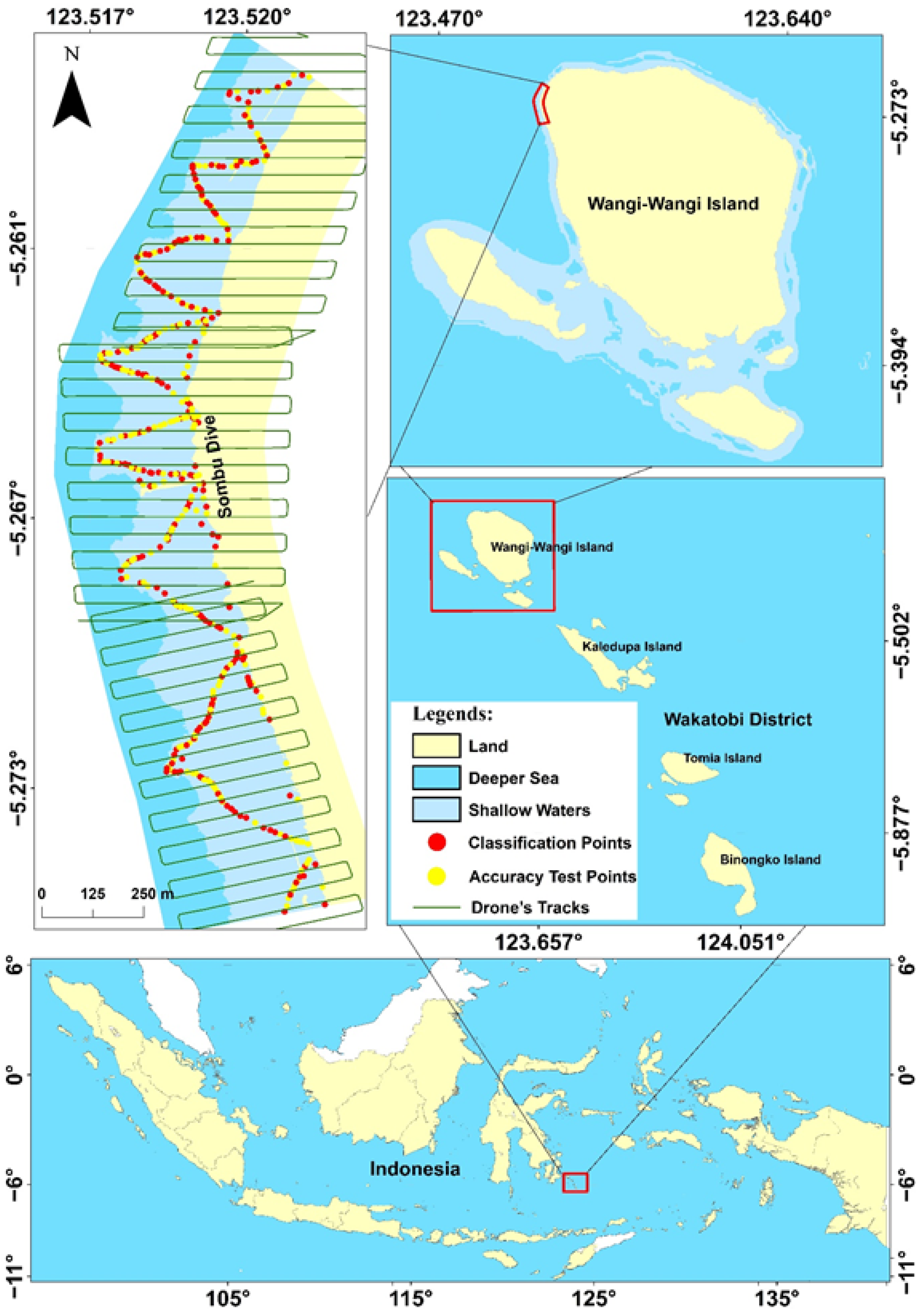
2.1. Study Area

The study was conducted in the region of Wangiwangi island waters, Wakatobi District, Southeast Sulawesi Province, Indonesia located along 5°15′22.6″–5°16′33.3″S and 123°31′11.5″–123°31′14.9″E (Figure 1).
The Wangiwangi island water is a unique shallow-water area with very high benthic habitat complexity and located in the coral triangle region or within the center of the world’s highest coral reef biodiversity [3,78,79,80]. Wangiwangi island is one of the 4 major islands in Wakatobi district (Wangiwangi, Kaledupa, Tomia, and Binongko islands) [4,5]. Within the Wakatobi region, about 25 pristine coral reef clusters were found, consisting of 396 coral species from 599 world coral species [81], with types of coral reefs including fringing reefs, patch reefs, barrier reefs, and ring coral (atoll) [5,6,78].
Drone image acquisition and field collection data for benthic habitat mapping were conducted on 29 March–2 April 2017 with flying tracks perpendicular to the coastline as shown in the upper left in Figure 1. A total of 434 field data transects with 50 × 50 cm spatial resolution were collected in which 217 points for classification purposes (red dots in upper left in Figure 1) and 217 points for accuracy test purposes (yellow dots in upper left in Figure 1).
When collecting field data in each station, the transect (50 × 50 cm) was always placed within the homogenous subtract shallow-water benthic habitat. For example, a live coral station of shallow-water benthic habitat, then the transect was placed in the center of a region of homogenous live coral of shallow-water benthic habitat. This was intended to reduce error of mismatch coordinate between in situ and the drone measurement, because we did not have access for a high precision GPS (up to ≤5 cm or mm).

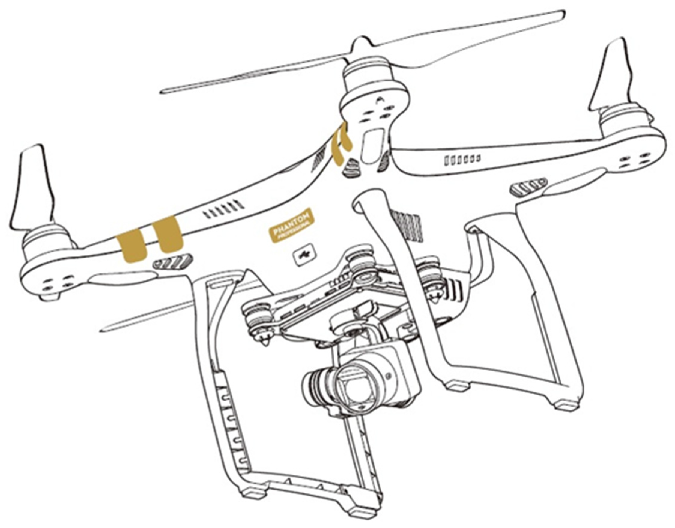
2.2. Tools and Materials

Tools and materials used in this study were GPS Trimble GeoExplores 6000 series (with accuracy of +/- 50 cm), Snorkeling tools, quadrate transects, underwater Canon PowerShot D20 camera, underwater stationaries, and waterproof plastics.
Drone images were taken using DJI Phantom 3 Professional made in Dà-Jiāng Innovations Science and Technology/DJI. The DJI Phantom 3 Professional is a DJI quadcopter generation that has more complete components from the previous generation (Figure 2). The DJI Phantom 3 Professional sensor was a built-in sensor from DJI or a standard Red-Green-Blue (RGB) sensor/camera. A standard RGB camera captures the visible electromagnetic spectrum of red, green, and blue lights. This sensor produces an RGB image and captures an image similar to what is seen with the human eye [82,83]. The DJI Phantom 3 Professional can fly up to 120 m with a maximum speed of 16 m/s, a maximum flying time of 23 min, and a FOV lens of 94° 20 mm (Table 1). Two software applications were used during deployment i.e., DJI GO application for basic settings and DroneDeploy application for the aerial photo acquisition processes. DroneDeploy is a mapping application using UAVs to make it easier for acquiring aerial photos automatically. Both applications were run via a mobile phone or tablet device with the Android or iOS operating system.

2.3. Benthic Habitat Data Collection

Ground truth habitat (GTH) surveys were conducted to collect benthic habitat data or information employing 50 × 50 cm transect (Figure 3) with direct visual observation and quadrat photo transect technique. The distribution of sampling stations used stratified random sampling method and evenly spread to obtain well-represented data from all benthic habitat objects within the study region [21,24,85,86].
The field object classification was based on the dominant percentage coverage of object(s) in each transect, and the coordinate location of each transect was taken using GPS at the center of the transect. If within a transect consisted of two major elements of benthic habitats, then the name of the transect was called based on the two-element starting with the more dominant element; for instance, a transect consisted of rubble (dominant) + seagrass, then we called this transect a rubble dominant + seagrass (R + S) transect. The threshold for the dominant element of benthic habitat was when the element occupied (covered) more than 50% of the transect space. The coordinates were later used as a reference for the region of interest (RoI) in the image classification process. Some of them were used as data to test the accuracy of the image classification results.
The description or naming of benthic habitat classes was determined based on the composition of the dominant benthic habitat cover which was entirely constructed by one or several components of shallow water benthic habitat. The classification scheme in this study consisted of 2 levels i.e., classification scheme level 1 (reef level class) and classification scheme level 2 (benthic habitat class).

2.4. Drone Image Acquisition

An aerial photo quality depends on environmental conditions such as wind, current, wave, cloud coverage, and sun intensity. Good quality of an aerial photo will be found during the relatively low wind speed, calm water conditions (small wave to calm water and low current speed), clear sky, and no sun glint. The presence of sun glint can cause unclear image or misalignment in the photogrammetric workflow. [87] revealed that in order to avoid or minimize the presence of sun glint in the aerial photo acquisition process, the aerial photo acquisition could be carried out in the morning at 07.00–08.00 AM. During these hours, generally the water environment is relatively calm and windless. In addition, the effect of sun glint can be controlled based on a combination of location conditions and low sun angles around 20–25° [88,89].
In this study, the processes of acquiring aerial photos were carried out in the morning at 07.00–08.00 AM local time to avoid sun glint with a camera angle perpendicular to the object surface, with relatively calm water condition, clear sky, and relatively low wind speed.
The drone was placed at an altitude of 120 m above the water surface. Drone images (photos) were captured with 80% sidelap and frontlap settings with a maximum flight speed of 15 m/s. The coverage area was adjusted to the research location and the drone battery capabilities. All aerial photo acquisitions were completed on 29–30 March and 2 April 2017.
In total 1274 aerial photos were taken along the flying tracks in the study region with 80% overlap both sidelap and frontlap.

2.5. Orthophoto Digital Processes

All aerial photos acquired by the drone at the study area were combined (orthomosaic) using Agisoft Photoscan software to produce single photo/image orthophoto or drone image. The orthomosaic processes of all aerial photos were carried out by several processing steps i.e., (1) add photo (to combine all photos that need to be included); (2) photo alignment (matching identical point cloud in two or more photos and build a sparse point cloud model); (3) optimize camera alignment (a process of optimizing the accuracy of camera parameters and correcting any distortion in photos); (4) build dense cloud (to build and combine the same set of point cloud on two or more in the number of thousands to millions of dense point cloud); (5) build mesh (to connect the surface of each photo based on the dense point cloud to build a 3D model); (6) build texture (to build texture and color formation of objects according to photos or 3D physical models of the features in the photo coverage area); (7) building orthomosaic (to produce orthophoto image in 2D formation) and (8) export orthomosaic (export orthophoto images for further classification or analysis). These processes were carried out sequentially to produce an orthophoto image or drone image.
The resulting drone image was an image that had been equipped with geographic information (georeferenced), considering that all the acquired aerial photos had been equipped with geographic information in the form of coordinate points and the geographic information was inputted in the orthomosaic process. The resulting drone image was used in the image classification process to classify the shallow water benthic habitat map.

2.6. Geometric Correction

The image geometry must be corrected to match the map used with the selected coordinate system, so that the image can be appropriately identified or the points observed in the field can be found correctly in the image [90]. Usually, in geometric correction, GCP (ground control points) were used to adjust the image position to the actual position in the field. Furthermore, rectification was carried out to correct geometric errors in the image. Geometric correction for the drone image was conducted automatically during orthomosaic processes because georeferenced or geographic information was automatically inputted during the processes.

2.7. Image Classification

To produce benthic habitat classification, object-based image classification (OBIA) method was used in this study. The OBIA method is a classification method developed with object segmentation and analysis processes or an image classification process based on its spatial, spectral and temporal characteristics, resulting in image objects or segments which are then used for classification [30,91].
Segmentation is a concept for building objects or segments from pixels into the same object or segment [92]. In this study, we used the multiresolution segmentation (MRS) algorithm. This algorithm started with a single pixel and combined neighboring segments until the heterogeneity threshold was reached. In the segmentation process using the MRS algorithm, there were three important parameters i.e., shape, compactness, and scale. Shape functions to regulate the spectral homogeneity and shape of the object in relation to the digital value influenced by color. Compactness plays a role in balancing or optimizing the compactness and smoothness of objects in defining objects between smooth boundaries and compact edges. Scale functions to adjust the size of the object that can be adjusted according to user needs based on the level of detail. The values used in the shape and compactness parameters ranged from 0–1, while the scale value was an abstraction in determining the maximum heterogeneity value to generate an object. Therefore, there were no standard provisions regarding the standard parameter values in object-based classification [24,93,94].
Multiscale segmentation was applied with several different scales at level 1 (reef level) and level 2 (benthic habitat). At level 1 (reef level i.e., land, shallow water, and deeper water map), we used the segmentation scale of 200 because this value produced the best map for reef level (land, shallow water, and deeper water map) visually than any other values (we used segmentation values of 1000, 900, 800, 700, 600, 500, 400, 300, 250, 200, 150 for try and errors and found the segmentation value of 200 produced the best map at the reef level). While at level 2, we used several different values for the optimization segmentation scale. At the segmentation stage, the shape and compactness parameter values used fixed values i.e., 0.1 and 0.5, respectively.
Segmentation scale optimization in the OBIA method showed that the segmentation scale could affect the accuracy of the image classification result [1]. The application of scale parameter optimization was only applied to level 2 (benthic habitat levels) in drone image using the MRS algorithm. The optimization values of the scale parameters used in the drone image were MRS 25, 50, 60, 70, and 100. To produce the best image result from the MRS optimizations, an accuracy test for the image was performed. The best accuracy scale was the scale used to produce the highest overall accuracy value of the image using the formula stated in the following sub-chapter. The best accuracy image was then used for final benthic habitats classification using eCognition software and employing several machine learning classification algorithms such as SVM, Bayes, KNN, and DT algorithms.

2.8. Benthic Habitat Classification Scheme

The classification scheme used in this study was based on one benthic habitat component or a combination of several benthic habitat components itself. The benthic habitat classification scheme was a structured system for determining habitat types into classes that can be defined based on ecological characteristics. The initial stage in mapmaking was to clearly identify the classes and describe their attributes. Classification schemes were used to guide habitat boundaries and definitions in the map-making process. This stage was important for map users in understanding how the classification system as a structure defined each class [95].
From the results of data collection on benthic habitats at the study region, 7 main components of shallow-water benthic habitats were found i.e., live coral, dead coral, seagrass, sand, algae, rubble, and intertidal rocks. The determination of the benthic habitat classification scheme was based on the dominant coverage of benthic habitat components obtained from field observations on the 50 × 50 cm transect both visually, supported by the use of quadratic transect photographs. The benthic habitat components, contained in each of the quadratic observation transect, were composed of a benthic habitat composition which was dominated by one benthic habitat component or a mixture of several benthic habitat components.
The next step was to determine the name (labeling) of each class of benthic habitat produced. Labeling was the final stage in the process of producing a shallow-water benthic habitat classification scheme. Based on the results of observations in the field at 434 observation stations (see Figure 1), there were 12 benthic habitat components in the study region (Figure 4). The names and descriptions of the 12 benthic habitat components were based on the dominant cover of benthic habitat at each observation point which was composed of one or more benthic habitat components. A single benthic class habitat such as algae means that in that station 100% algae were found. A mixture class of a benthic habitat such as live coral + dead coral meant that in the respective station a mixture benthic habitat composition of live coral and dead coral were found, where live coral do-minated the composition. Of the 12 components of benthic habitat found in the study region, we constructed two benthic habitat classification schemes i.e., 12 and 9 shallow-water benthic habitat classes. The twelve classes of benthic habitats were algae, intertidal rocks, live coral, live coral + dead coral, dead coral, seagrass, seagrass + sand, sand, sand + seagrass, sand + rubble, rubble, and rubble + seagrass. Meanwhile, nine classes of benthic habitats consisted of algae, intertidal rocks, live coral, dead coral, seagrass, seagrass + sand, sand, sand + seagrass, and rubble. The names, descriptions and codes of each benthic habitat class were presented in Table 2.
We reduced the number of classes from 12 to 9 to improve the classification map accuracy since several benthic habitat class types could produce similar reflectance signal such as sand (Sd) and sand + rubble (SdR). Therefore, these two classes were combined within one class i.e., sand (Sd) within the 9 class types. Live coral (LC) and live coral + dead coral (LCDC) classes, were combined to be live coral (LC) class within the 9 class types. While rubble (R) and rubble + seagrass (RS) were combined to be rubble (R) class within the 9 class types. The resulting classification schemes 12 and 9 shallow-water benthic ha-bitat classes were used in the drone image classification process.
The determination of the benthic habitat classification scheme has no standard provisions until today so that the designation of benthic habitat classes in this study was adjusted to the composition of the dominant benthic habitat constituents observed in the field. Several studies on determining the classification scheme for shallow water benthic habitats have been carried out and resulted in different classification schemes or the number of classes such as [92] developing a classification scheme from field observations at the detailed benthic coral reefs more than 15 classes mostly dominated by classes composed of more than one benthic component. The classification scheme has been developed hierarchically by [24] for mapping benthic habitats in the western Pacific on coral reef ecology produced 12 classes of benthic habitat classification schemes constructed from 9 types of benthic cover. [2] produced 12 benthic habitat classes, [20] produced six benthic habitats, [18] produced seven benthic habitat classes and [17] produced nine benthic ha-bitat classification schemes.

2.9. Accuracy Test

An accuracy test was carried out on all classified images to determine the accuracy of the applied classification technique. The common accuracy test performed on remote sensing classification results data was the confusion matrix. This was done by comparing the classified image to the actual class or object obtained from the field observations [18].
Accuracy test using confusion matrix refers to [86] which consists of overall accuracy (OA), producer (PA), and user accuracy (UA). The formulas to calculate the level of accuracy for both OA, PA, and UA were presented in the following equations:
OA = i = 1 k n i i n
PA j = n j j n + j  
UA i = n i i n i +
where, OA = overall accuracy, PA = producer accuracy, UA = user accuracy, n = number of observations, nii = number of observations in column i and row i, and njj = number of observations in column j and row j. n+j = the number of samples classified into category of j, ni+ = the number of samples classified into category i.

3. Result and Disscussion

3.1. Digital Orthophoto

Overall, 1274 aerial photographs covering all study regions were observed. We later combine all these photographs through orthomosaic process to produce one high-quality of digital drone orthophoto.
The resulting digital orthophoto image was a georeferenced two-dimensional image. According to [96], in general, orthophoto images only produce two-dimensional display images that are equipped with X and Y coordinate information. The digital orthophoto image of the orthomosaic results in this study is shown in Figure 5.
Orthophoto image was produced through a repair process related to photo tilt, lens distortion, and relief displacement which were then eliminated or adjusted [96], and the process was carried out with certain stages and procedures to produce high quality image. The orthophoto image had a very high spatial resolution of 5.2 × 5.2 cm with total area of 106 ha or 1.06 km2. The resulting orthophoto was later used as data input in the shallow water benthic habitat classification processes.

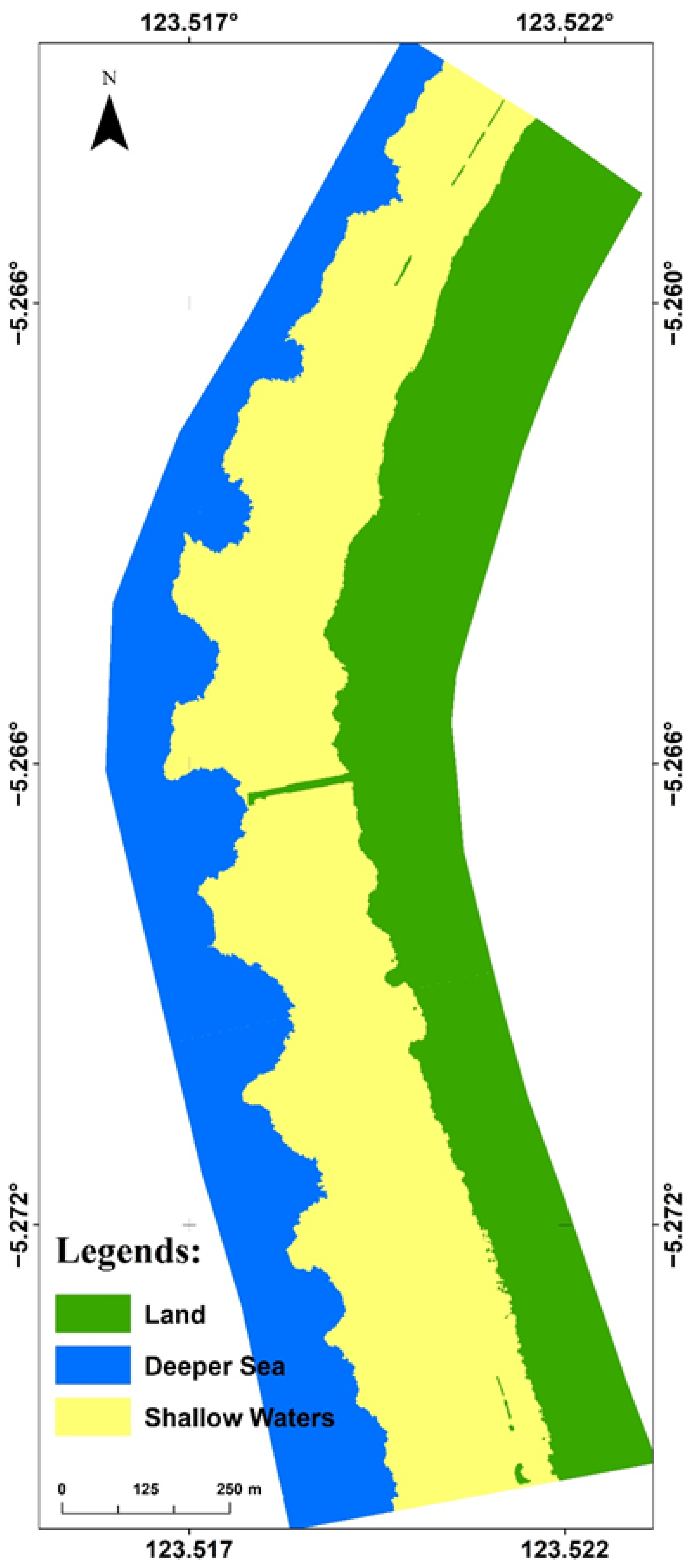
3.2. Image Classification Level 1 (Reef Level)

After conducting orthophoto digital processing using drone images, we performed an OBIA classification using several segmentation values. At level 1 (reef level), the best segmentation scale used was 200 and produced 12276 objects. From these 12276 objects, we classified into three classes i.e., land, shallow water, and deeper water (Figure 6). Based on the classification result in level 1 (reef level), we found that the total area of drone image was 106 Ha consisting of shallow-water class of 45.2 Ha, land class of 33.9 Ha, and deepwater class of 26.9 Ha (Figure 6).

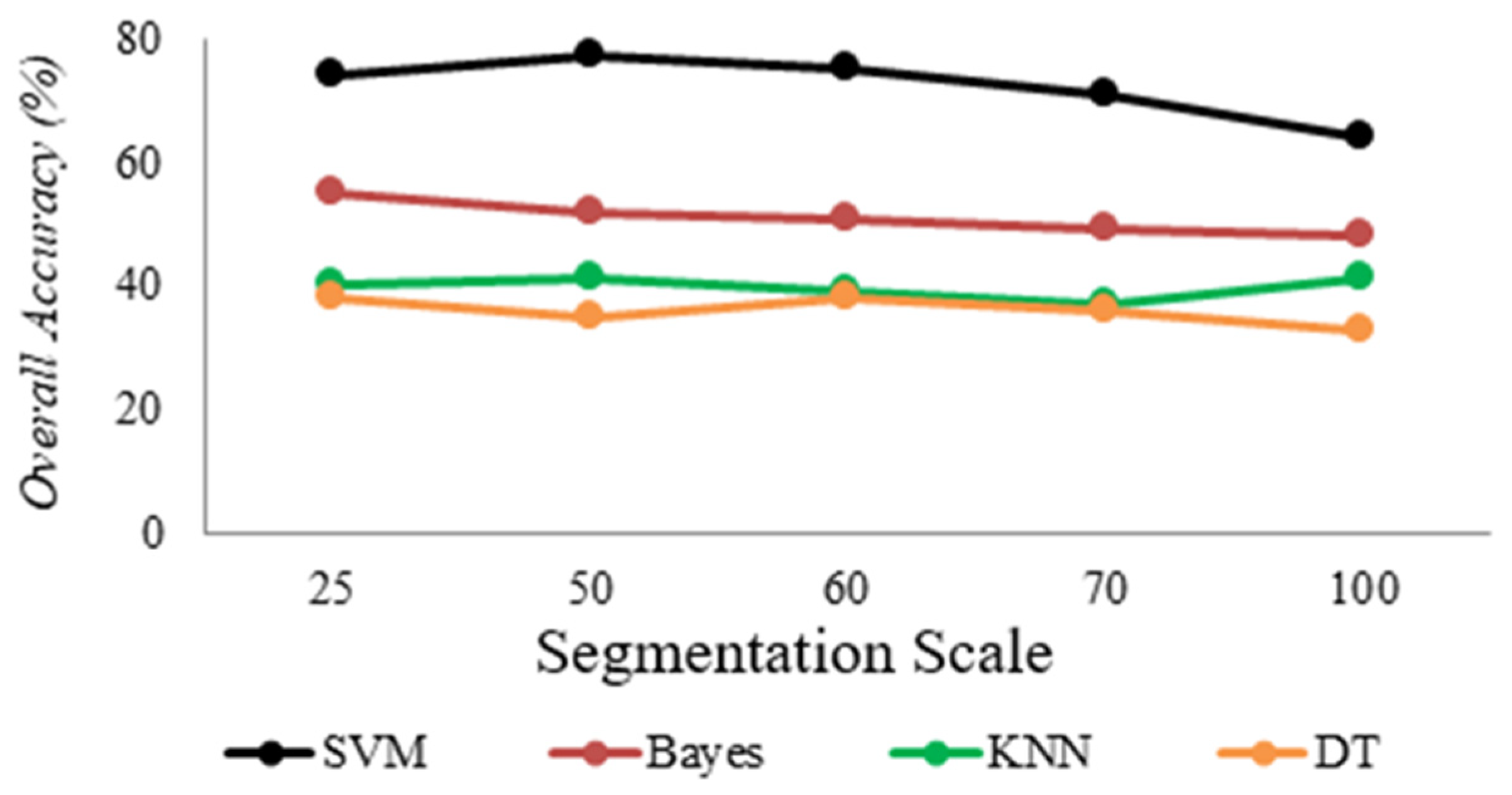
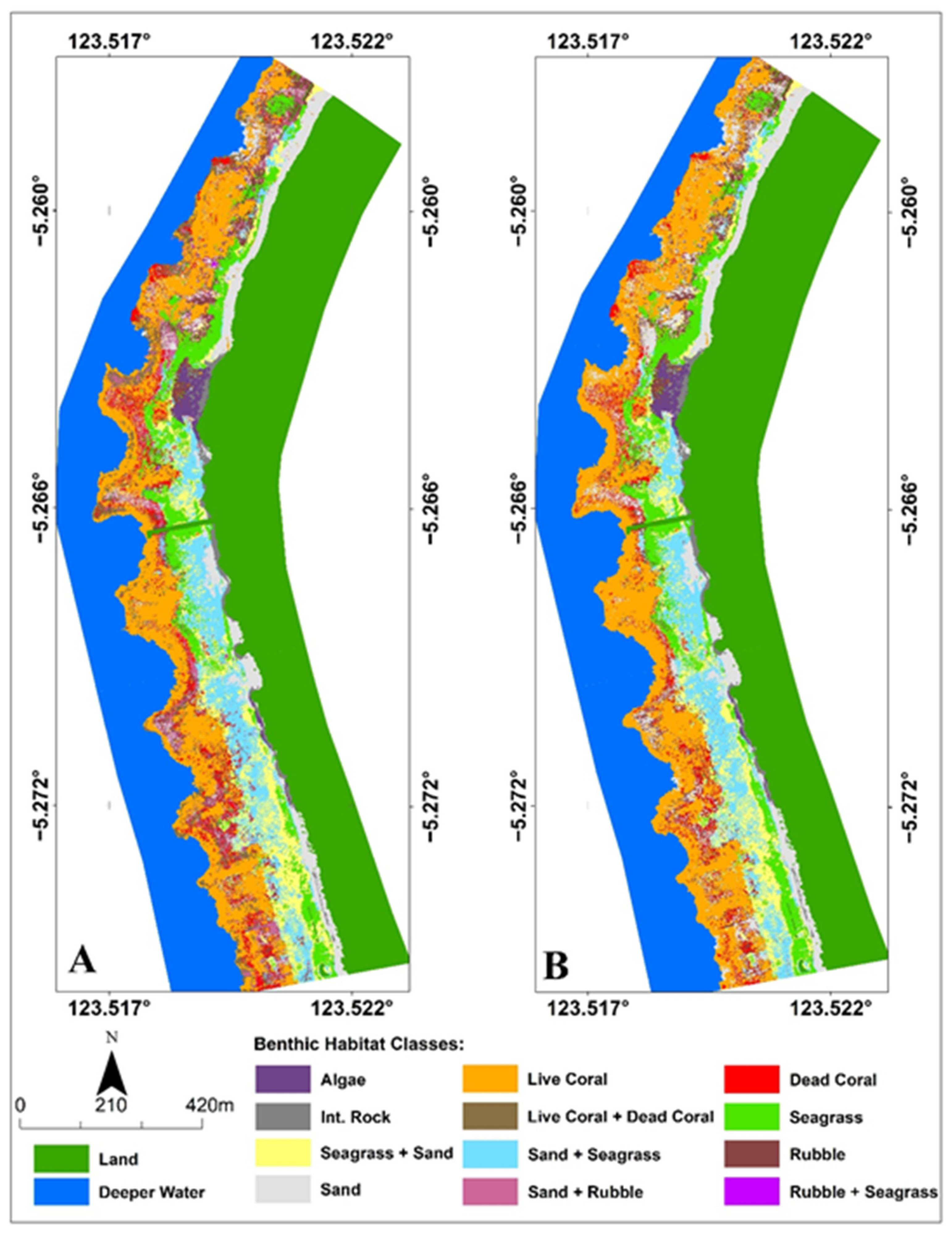
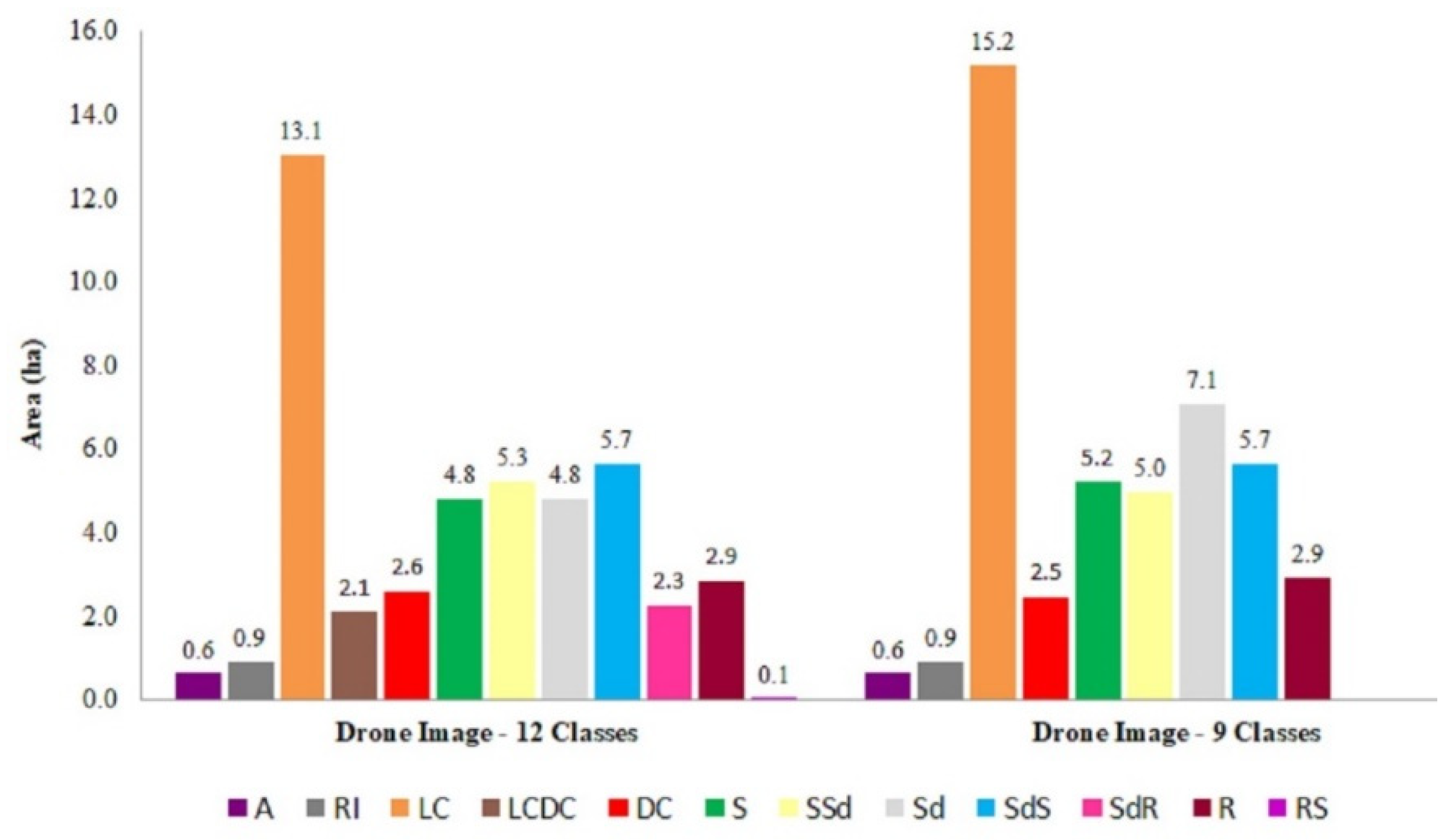
3.3. Image Classification Level 2 (Benthic Habitat Classification)

At level 2, the shallow-water class from level 1 classification, optimization was performed using MRS segmentation values of 25, 50, 60, 70, and 100 with the shape and compactness values using default (fix) values in the software i.e., 0.1 and 0.5, respectively (Figure 7). Results showed that the smaller the segmentation value applied, the higher the number of objects produced and also the smaller the shape or size of the object (Figure 7).
For the whole shallow-water region in level 1 classification, the multi-scale segmentation processes using segmentation values (scales) of 25, 50, 60, 70, and 100 were performed. We obtained as many as 320,788, 88,786, 73403, 49,514, and 27,632 objects, respectively. The results of segmentation scale optimization can be seen that the parameters of the segmentation scale greatly affected the process of forming objects in the image, both the number and shape of the object. [18] showed that segmentation scale could affect the shape, size, and number of objects produced. The number and size of objects formed in the image were based on the heterogeneity or complexity of an object at the research location (the shallow water benthic habitat). Areas that contained more heterogeneous objects in an image produced more objects than areas that had less heterogeneous objects [1]
The resulting objects or segments were then classified by several machine learning algorithms contained in the Cognition Developer software version 8.7 such as the support vector machine (SVM), decision tree (DT), Bayesian, and K-Nearest Neighbor (KNN) applying the shallow water benthic habitat classification scheme (see Table 2) as an input thematic layer. Of the total 434 field observation points, 217 observation points were used as input data (input thematic layer) in the classification process and the remaining 217 observation points were used as data for accuracy testing using confusion matrix. The input features in the level 2 classification process for drone image used the spectral/layer (RGB) values i.e., mean, standard deviation, and transformation value of Hue, Saturation, and Intensity (HSI).
The application of segmentation scale optimization on 12 benthic habitat classes (see Table 2) in the drone image, we obtained the highest accuracy of 77.4% on the segmentation value of 50 applying the SVM algorithm, while the lowest accuracy of 32.7% was obtained on the segmentation value of 100 applying DT algorithm (Figure 8).
For nine benthic habitat classes (see Table 2), the application of segmentation scale optimization produced the highest accuracy of 81.1% on the segmentation value of 50 with the SVM algorithm, while the lowest accuracy of 36.4% was obtained on the segmentation value of 100 with DT algorithm (Figure 9).
Based on the optimization results of the segmentation scale using the drone image in the 12 and 9 benthic habitat classes with the application of several classification algorithms, it was clear that the SVM algorithm produced the highest overall accuracy compared to other classification algorithms. This was in accordance with the results of previous research by [18] which mapped the benthic habitat of coral reefs using Landsat 8 OLI Satellite imagery with OBIA method employing several classification algorithms such as the SVM, random tree (RT), DT, Bayesian, and KNN algorithms. They found that the SVM algorithm produced the best overall accuracy of 73% for seven benthic habitat classes. [97] mapped benthic habitats with several classification algorithms such as MLC (maximum likelihood), SAM (spectral angular mapper), SID (spectral information divergence), and SVM, and they produced optimum accuracy values for the application of the SVM algorithm [98] also stated that the SVM algorithm in remote sensing had a good ability to handle small amounts of data and can produce better accuracy than other classification techniques. The main factor that affects the accuracy improvement using machine learning algorithms (SVM) was the ability to distinguish objects well from the use of data with unknown empirical probability characteristics [99].
To study in more detail on benthic habitats in the study region, maps of 12 and 9 classes of shallow-water benthic habitat applying the SVM algorithm with segmentation values of 50 were produced (Figure 10).
Based on Figure 10A, the total area of shallow-water benthic habitats within 12 classes was 45.2 Ha. From the 12 classes of benthic habitats, the live coral class (LC) dominated the shallow-water region with a total area of 13.1 Ha (28.98%), followed by sand + seagrass (SdS) of 5.7 Ha (12.61%), seagrass + sand (SSd) of 5.3 Ha (11.72%), seagrass (S) and sand (Sd) each of 4.8 Ha (10.62%). Meanwhile, the smallest area was the rubble + seagrass (RS) class with a total area of 0.1 Ha 0.2%) (Figure 11).
The total area for 9 classes of shallow-water benthic habitats was 45.1 Ha (Figure 10B). From the nine classifications of benthic habitats, the live coral (LC) also dominated the shallow-water region with a total area of 15.2 Ha (33.70%), followed by sand (Sd) of 7.1 Ha (15.74%), sand + seagrass (SdS) of 5.7 Ha (12.64%), sand of 5.2 Ha (11.53%), and seagrass + sand (SSd) of 5.0 Ha (11.08%). While the smallest area was the algae class (A) with a total area of 0.6 Ha (1.33%) (Figure 10B and Figure 11). The increase of live coral (LC) percentage coverage in the 9 classes map occurred because within the 9 classes map the live coral (LC) and live coral + dead coral (LC + DC) were combined become one class i.e., live coral (LC) class. The sand class coverage also increased within the 9 classes because the sand (Sd) and sand + rubble (SdR) were combined become one class i.e., the sand type.
Based on the accuracy-test using an error matrix (confusion matrix), we found an overall accuracy (OA) of 77.4% for the 12 classes of benthic habitat classification. For producer accuracy (PA) and user accuracy (UA) values, the accuracy ranges from 20–100% (Table 3). From these results, several benthic habitat classes can be mapped very well, especially in the algae class (A) which produces the highest UA value of 100%. Live coral (LC), sand (Sd), dead coral (DC), rubble (R), and intertidal rock (IR) were benthic habitat elements that can be mapped with high user accuracy (UA) with the range of 80–93% (Table 3). Meanwhile, other benthic habitat classes met the minimum requirement for mapping (UA > 60%) were sand + seagrass (SdS), live coral + dead coral (LCDC), and seagrass + sand (SSd) with UA values of 63–71%. The other two benthic habitat elements that had not been mapped properly were the sand + rubble (Sd + R) with UA value of 56% and rubble + seagrass (R + S) with UA value of 50%.
The low accuracy value in several benthic habitat classes was strongly influenced by the complexity of the benthic habitat in the study region and the number of observation points in each benthic habitat class. The dominant reflectance signal from one element of mixture benthic habitats to another such as sand + seagrass (SdS), live coral + dead coral (LCLD), sand + rubble (Sd + R), and rubble + seagrass (R + S) can produce low user accuracy value. The first element of these mixture benthic habitats dominated reflectance signal from the second element benthic habitat and therefore the reflectance signal from the second element of benthic habitat may not be detected by satellite. In addition, the spectral similarity between habitat classes cannot be avoided by classification algorithms, especially in benthic habitat classes composed of two benthic habitat components. Another factor affecting this accuracy map was the GPS accuracy used during field data collection and satellite image spatial resolution [17]. In this study, we used GPS Trimble GeoExplores 6000 series that has an accuracy level within 50 cm. Ref. [89] stated that the minimum overall accuracy requirement for mapping benthic habitat was 60%. Therefore, the benthic habitat classification of the drone image in this study was good enough for the purpose classification mapping.
Based on the low user accuracy value results in mapping live coral + dead coral (LCDC), sand + rubble (Sd + R), and rubble + seagrass (R + S) within the 12 benthic habitat classes, we therefore eliminated these mixture benthic habitat classes and produced a map for nine class benthic habitats. After performing confusion matrix analyses, for the nine classes of benthic habitat classification, we found an overall accuracy of 81.1% (increased by 3.7% from the twelve classes of benthic habitat classification) (Table 4). This showed that the number of object classes greatly affected the accuracy of the classification results, where the smaller number of classes (9 classes) resulted in a higher overall accuracy compared to the larger number of classes (12 classes). This was in accordance with the research results of [26] who applied several numbers of classes to produce an overall accuracy that decreased with the increase in the number of classes used i.e., an average accuracy of 77% (4–5 classes), 71% (7–8 classes), 56% (9–11 classes), and 53% (>13 classes) in Landsat and IKONOS imageries.
Some misclassifications within the 9 classes of benthic habitat map between field observations and satellite detections were observed between dead coral (DC) and live coral (LC) (4 of 18 = 22%), rubble (R) and live coral (LC) (5 of 23 = 22%), seagrass (S) and sand + seagrass (S + SSd) (3 of 29 = 29%), rubble (R) and sand (Sd) (3 of 23 = 13%), sand (Sd) and rubble (R) (3 of 38 = 8%) (Table 4). The results showed that misclassification mostly occurred within the benthic habitat with closely similar characteristics.
The mapping of shallow-water benthic habitats has been widely carried out using the object-based classification method (OBIA). The use of the OBIA method has also been shown to improve shallow-water benthic habitat mapping accuracy. [94] mapped 11 benthic classes using Quickbird images with fuzzy logic algorithms and contextual editing resulting in an accuracy of 83.5%. [24] mapped 12 benthic habitat classes using Quickbird-2 imagery and produced a mapping accuracy of 52–75%. [18] conducted mapping on seven classes of benthic habitat on coral reefs using Landsat 8 OLI with the SVM algorithm and produced an overall accuracy of 73%. [17] mapped nine benthic habitat classes using Worldview-2 imagery with the SVM algorithm and produced an overall accuracy of 75%. In this study, mapping with drone image was carried out using 12 and 9 benthic habitat classes which produced the highest overall accuracy of 77.4% and 81.1%, respectively, employing the SVM algorithm. [100] mapped the submerged habitat using the drone type FPV Raptor 1.6m RxR and Canon SX 220 camera on five benthic habitat classes using the OBIA method with the SVM algorithm and produced an overall accuracy of 87.1%. The difference in mapping accuracy from several previous studies was due to differences in classification algorithms, the type of image used, the number of classes or complexity of benthic habitats, and the number of field observation points. Ref. [101] assessed the accuracy of benthic habitat mapping using Sentinel-2 satellite data with 10 × 10 m spatial resolution acquired on 4 April 2017 (the closest time of the satellite data available with the drone data acquisition in this study) within the similar location, similar number and locations of field measurements, similar number of benthic habitat classes (12 and 9 classes), and similar method for mapping classification (OBIA method employing SVM, Random Tree (RT), DT, Bayesian, and KNN algorithms) [101]. The result showed that based on OBIA method and SVM algorithm with an optimum segmentation scale of 2, shallow-water benthic habitat produced the highest overall accuracy of 60.4% and 64.1% for 12 and 9 object classes. Therefore, compared to this study results, the overall accuracy was increase of 17% both for 12 and 9 object classes of benthic habitat when classified with a similar method using the drone image.
Based on this study result, the drone technology can be used as an alternative in providing images with very high spatial resolution to map benthic habitats with high habitat complexity. However, the use of UAV technology for benthic habitat mapping requires further development and research, considering that the resulting UAV image in this study only provides the RGB bands with low spectral resolution. In addition, what needs to be considered in the use of drone technology for mapping shallow-water benthic habitats is related to the process of acquiring aerial photographs as well as water and weather conditions at the study site so that it can produce a better image.
The drone technology, in general, produced relatively higher accuracy for shallow-water benthic habitats compared to other high spatial resolution satellites even though the total class (type) of shallow-water benthic habitats was equal or less than 12 classes such as [17] for 9 classes of benthic habitats using Worldview-2 with SVM algorithm and produced the best accuracy of 75%, [18] for coral reef habitat map using Landsat 8 OLI with OBIA and SVM algorithm with total accuracy of 73% for 7 classes, [24] for 12 classes of benthic habitats using Quickbird-2 produced the maximum accuracy of 75%, and [101] for 12 classes of coral reef benthic habitats using Landsat 8 OLI satellite imagery with OBIA and SVM algorithms produced total accuracy of 73%. Meanwhile, [90] mapped 11 classes of benthic habitats using Quickbird image with fuzzy logic algorithm and contextual editing produced total accuracy of 83.5%. [100] mapped for 5 classes benthic habitats using drone with OBIA and SVM algorithm produced accuracy of 87.1%. The last two mapping benthic habitat results produced better accuracy than this study probably because the total classes of benthic habitat in the last two study were less than the total classes in this study and also the type of benthic habitat classes may be different one of another.
Some factors affecting the accuracy map of the drone image were the flying time for capturing image and the camera angle in respect to the water surface. In this study, the drone flying time was at 8:00 am local time with camera angle perpendicular to the water surface. The drone flying time was chosen at 8:00 a.m. local time due to fact that based on trial drone flying time at 9:00 a.m., 10:00 a.m., or 11:00 a.m., 1:00 p.m., 2:00 p.m., and 3:00 p.m. all images captured by the drone were fill up with the sunglint effect. Meanwhile, the total irradiances from the sun reached the water column especially on the blue and green wavelengths were relatively lower at 8:00 a.m. than at 9:00 a.m., 10:00 a.m., 11:00 a.m., 1:00 p.m., 2:00 p.m., and 3 p.m. Therefore, the relatively low signal especially in the blue and green wavelengths at 8:00 a.m. from the water column may affect the clarity of the shallow-water benthic habitat characteristics and later affected the accuracy of the shallow-water benthic habitats map classifications.
To increase the accuracy of the drone image classification, further research may also be focused on flying time for the drone capturing image and the drone camera angle in respect to the water surface. To avoid sunglint effect and to increase irradiance signals received by the water column, the drone flying time may be chosen at 10–11 a.m. or 1–2 p.m. local time with the drone camera angle with respect to the water column at 30° or 45°. [102] stated that variations in remote sensing reflectance from water column can be attributed to a variety of environmental factors such as Sun angle, cloud cover, wind speed, and viewing geometry; however, wind speed was not the major source of uncertainty. According to [102] the best viewing angle of the instrument with respect to the vertical line of the instrument and the water column was 45°.

4. Conclusions

Using drone technology, we can map shallow-water benthic habitat with relatively high overall accuracy values of 77.4% and 81.1% for 12 and 9 object classes using OBIA method with 50 segmentation scale and applying SVM classification algorithm. This result improved overall accuracy up to 17% in mapping benthic habitats using Sentinel-2 satellite data within the similar region, similar classes, and similar method of classification analyses.
The algae class (A) produced the highest user accuracy (UA) value of 100%, while sand + rubble (Sd + R) and rubble + seagrass (R + S) produced user accuracy (UA) below the minimum requirement for an acceptable benthic habitat map with UA value of 56% and 50%, respectively. Misclassification mostly occurred within benthic habitat elements with closely similar characteristics.
Total area of shallow-water benthic habitats detected by the drone image in the study region was 45.1 Ha within the 9 classes benthic habitats. Live coral (LC) dominated the shallow-water region with a total area of 15.2 Ha (33.70%), followed by sand (Sd) of 7.1 Ha (15.74%), sand + seagrass (SdS) of 5.7 Ha (12.64%), sand of 5.2 Ha (11.53%), and seagrass + sand (SSd) of 5.0 Ha (11.08%), while the smallest area was the algae class (A) with a total area of 0.6 Ha (1.33%).

Author Contributions

Conceptualization, B.N.; Field data collection, L.O.K.M.; Data analyses, B.N. and L.O.K.M.; Data curation, L.O.K.M.; Funding acquisition, B.N., N.H.I.; Writing-original draft, B.N.; Writing-review and editing, B.N., N.H.I. and J.P.P.; Project administration, B.N. and J.P.P. All authors have read and agreed to the published version of the manuscript.

Funding

This research was funded by the Directorate Research Strengthening and Development, Ministry of Research and Technology/National Research and Innovation Agency, Republic of Indonesia with grant No. 1/E1/KP.PTNBH/2020 dated 18 March 2020 and Research Implementation and Assignment Agreement Letter for Lecturers of the IPB University on Higher Edu-cation Selected Basic Research for 2020 Fiscal Year with No.: 2549/IT3.L1/PN/2020 dated 31 March 2020 and addendum contract No.: 4008/IT3.L1/PN/2020 dated 12 May 2020, the Universiti Teknologi Malaysia-RUG Iconic RA Research Grant (Vot 09G73).

Institutional Review Board Statement

Not applicable.

Informed Consent Statement

Not applicable.

Data Availability Statement

All data generated or analyzed during this study are included in this article and available on request from the corresponding author.

Acknowledgments

This research was supported by the Directorate Research Strengthening and Development, Ministry of Research and Technology/National Research and Innovation Agency, Republic of Indonesia with grant No. 1/E1/KP.PTNBH/2020 dated 18 March 2020 and Research Implementation and Assignment Agreement Letter for Lecturers of the IPB University on Higher Education Selected Basic Research for 2020 Fiscal Year with No.: 2549/IT3.L1/PN/2020 dated 31 March 2020 and addendum contract No.: 4008/IT3.L1/PN/2020 dated 12 May 2020, and the Universiti Teknologi Malaysia-RUG Iconic RA Research Grant (Vot 09G73). Special thanks go the head of the public works and mining department, Wakatobi district for the assistance of tools and facilities during the field data collection. We would also like to acknowledge reviewers who provided some comments and inputs to improve this paper.

Conflicts of Interest

The authors declare no conflict of interest.

References

  1. Anggoro, A.; Siregar, V.P.; Agus, S.B. Geomorphic zones mapping of coral reef ecosystem with OBIA method, case study in Pari Island. J. Penginderaan Jauh 2015, 12, 1–12. [Google Scholar]
  2. Zhang, C.; Selch, D.; Xie, Z.; Roberts, C.; Cooper, H.; Chen, G. Object-based benthic habitat mapping in the Florida Keys from hyperspectral imagery. Estuar. Coast. Shelf Ser. 2013, 134, 88–97. [Google Scholar] [CrossRef]
  3. Wilson, J.R.; Ardiwijaya, R.L.; Prasetia, R. A Study of the Impact of the 2010 Coral Bleaching Event on Coral Communities in Wakatobi National Park; Report No.7/12; The Nature Conservancy, Indo-Pacific Division: Sanur, Indonesia, 2012; 25p. [Google Scholar]
  4. Suyarso; Budiyanto, A. Studi Baseline Terumbu Karang di Lokasi DPL Kabupaten Wakatobi; COREMAP II (Coral Reef Rehabilitation and Management Program)-LIPI: Jakarta, Indonesia, 2008; 107p. [Google Scholar]
  5. Anonim. Coral reef rehabilitation and management program. In CRITC Report: Base line study Wakatobi Sulawesi Tenggara; COREMAP: Jakarta, Indonesia, 2001; 123p. [Google Scholar]
  6. Balai Taman Nasional Wakatobi. Rencana pengelolaan taman nasional Wakatobi Tahun 1998–2023; Proyek kerjasama departemen kehutanan PHKA balai taman nasional Wakatobi, Pemerintah Kabupaten Wakatobi; The Nature Conservancy dan WWF-Indonesia: Bau-Bau, Indonesia, 2008. [Google Scholar]
  7. Haapkyla, J.; Unsworth, R.K.F.; Seymour, A.S.; Thomas, J.M.; Flavel, M.; Willis, B.L.; Smith, D.J. Spation-temporal coral disease dynamics in the Wakatobi marine national park. South-East Sulawesi Indonesia. Dis. Aquat. Org. 2009, 87, 105–115. [Google Scholar] [CrossRef] [Green Version]
  8. Haapkyla, J.; Seymour, A.S.; Trebilco, J.; Smith, D. Coral disease prevalence and coral health in the Wakatobi marine park, Southeast Sulawesi, Indonesia. J. Mar. Biol. Assoc. 2007, 87, 403–414. [Google Scholar] [CrossRef]
  9. Crabbe, M.J.C.; Karaviotis, S.; Smith, D.J. Preliminary comparison of three coral reef sites in the Wakatobi marine national park (S.E. Sulawesi, Indonesia): Estimated recruitment dates compared with discovery Bay, Jamaica. Bull. Mar. Sci. 2004, 74, 469–476. [Google Scholar]
  10. Turak, E. Coral diversity and distribution. In Rapid ecologica assessment, Wakatobi National Park; Pet-Soede, L., Erdmann, M.V., Eds.; TNC-SEA-CMPA; WWF Marine Program: Jakarta, Indonesia, 2003; 189p. [Google Scholar]
  11. Crabbe, M.J.C.; Smith, D.J. Comparison of two reef sites in the Wakatobi marine national park (S.E. Sulawesi, Indonesia) using digital image analysis. Coral Reefs 2002, 21, 242–244. [Google Scholar]
  12. Unsworth, R.K.F.; Wylie, E.; Smith, D.J.; Bell, J.J. Diel trophic structuring of seagrass bed fish assemblages in the Wakatobi Marine National Park, Indonesia. Estuar. Coast. Shelf Sci. 2007, 72, 81–88. [Google Scholar] [CrossRef]
  13. Ilyas, T.P.; Nababan, B.; Madduppa, H.; Kushardono, D. Seagrass ecosystem mapping with and without water column correction in Pajenekang island waters, South Sulawesi. J. Ilmu Teknol. Kelaut. Trop. 2020, 12, 9–23. (In Indonesian) [Google Scholar] [CrossRef]
  14. Pragunanti, T.; Nababan, B.; Madduppa, H.; Kushardono, D. Accuracy assessment of several classification algorithms with and without hue saturation intensity input features on object analyses on benthic habitat mapping in the Pajenekang island waters, South Sulawesi. IOP Conf. Ser. Earth Environ. Sci. 2020, 429, 012044. [Google Scholar] [CrossRef]
  15. Wicaksono, P.; Aryaguna, P.A.; Lazuardi, W. Benthic habitat mapping model and cross validation using machine-learning classification algorithms. Remote Sens. 2019, 11, 1279. [Google Scholar] [CrossRef] [Green Version]
  16. Al-Jenaid, S.; Ghoneim, E.; Abido, M.; Alwedhai, K.; Mohammed, G.; Mansoor, S.; Wisam, E.M.; Mohamed, N. Integrating remote sensing and field survey to map shallow water benthic habitat for the Kingdom of Bahrain. J. Environ. Sci. Eng. 2017, 6, 176–200. [Google Scholar]
  17. Anggoro, A.; Siregar, V.P.; Agus, S.B. Multiscale classification for geomorphic zone and benthic habitats mapping using OBIA method in Pari Island. J. Penginderaan Jauh 2017, 14, 89–93. [Google Scholar]
  18. Wahiddin, N.; Siregar, V.P.; Nababan, B.; Jaya, I.; Wouthuyzend, S. Object-based image analysis for coral reef benthic habitat mapping with several classification algorithms. Procedia Environ. Sci. 2015, 24, 222–227. [Google Scholar] [CrossRef] [Green Version]
  19. Zhang, C. Applying data fusion techniques for benthic habitat mapping. ISPRS J. Photogram. Remote Sens. 2014, 104, 213–223. [Google Scholar] [CrossRef]
  20. Siregar, V.; Wouthuyzen, S.; Sunuddin, A.; Anggoro, A.; Mustika, A.A. Pemetaan habitat dasar dan estimasi stok ikan terumbu dengan citra satelit resolusi tinggi. J. Ilmu Teknol. Kelaut. Trop. 2013, 5, 453–463. [Google Scholar]
  21. Siregar, V.P. Pemetaan Substrat Dasar Perairan Dangkal Karang Congkak dan Lebar Kepulauan Seribu Menggunakan Citra Satelit QuickBird. J. Ilmu Teknol. Kelaut. Trop. 2010, 2, 19–30. [Google Scholar]
  22. Selamat, M.B.; Jaya, I.; Siregar, V.P.; Hestirianoto, T. Aplikasi citra quickbird untuk pemetaan 3D substrat dasar di gusung karang. J. Imiah Geomatika 2012, 8, 95–106. [Google Scholar]
  23. Selamat, M.B.; Jaya, I.; Siregar, V.P.; Hestirianoto, T. Geomorphology zonation and column correction for bottom substrat mapping using quickbird image. J. Ilmu Teknol. Kelaut. Trop. 2012, 2, 17–25. [Google Scholar]
  24. Phinn, S.R.; Roelfsema, C.M.; Mumby, P.J. Multi-scale, object-based image analysis for mapping geomorphic and ecological zones on coral reefs. Int. J. Remote Sens. 2011, 33, 3768–3797. [Google Scholar] [CrossRef]
  25. Shihavuddin, A.S.M.; Gracias, N.; Garcia, R.; Gleason, A.; Gintert, B. Image-based coral reef classification and thematic mapping. Remote Sens. 2013, 5, 1809–1841. [Google Scholar] [CrossRef] [Green Version]
  26. Andréfouët, S.; Kramer, P.; Torres-Pulliza, D.; Joyce, K.E.; Hochberg, E.J.; Garza-Pérez, R.; Mumby, P.J.; Riegl, B.; Yamano, H.; White, W.H. Multi-site evaluation of IKONOS data for classification of tropical coral reef environments. Remote Sens. Environ. 2003, 88, 128–143. [Google Scholar] [CrossRef]
  27. Mumby, P.J.; Edwards, A.J. Mapping marine environments with IKONOS imagery: Enhanced spatial resoltion can deliver greater thematic accuracy. Remote Sens. Environ. 2002, 82, 48–257. [Google Scholar] [CrossRef]
  28. Mumby, P.J.; Clark, C.D.; Green, E.P.; Edwards, A.J. Benefits of water column correction and contextual editing for mapping coral reefs. Int. J. Remote Sens. 1998, 19, 203–210. [Google Scholar] [CrossRef]
  29. Malthus, T.J.; Mumby, P.J. Remote sensing of the coastal zone: An overview and priorities for future research. Int. J. Remote Sens. 2003, 24, 2805–2815. [Google Scholar] [CrossRef]
  30. Wang, L.; Sousa, W.P.; Gong, P. Integration of object-based and pixel-based classification for mapping mangroves with IKONOS imagery. Int. J. Remote Sens. 2004, 25, 5655–5668. [Google Scholar] [CrossRef]
  31. Pádua, L.; Vanko, T.; Hruška, J.; Adão, T.; Sousa, J.J.; Peres, E.; Morais, R. UAS, sensors, and data processing in agroforestry: A review towards practical applications. Int. J. Remote Sens. 2017, 38, 2349–2391. [Google Scholar] [CrossRef]
  32. Castillo-Carrión, C.; Guerrero-Ginel, J.E. Autonomous 3D metric reconstruction from uncalibrated aerial images captured from UAVs. Int. J. Remote Sens. 2017, 38, 3027–3053. [Google Scholar] [CrossRef]
  33. Bazzoffi, P. Measurement of rill erosion through a new UAV-GIS methodology. Ital. J. Agron. 2015, 10, 695. [Google Scholar] [CrossRef] [Green Version]
  34. Brouwer, R.L.; De Schipper, M.A.; Rynne, P.F.; Graham, F.J.; Reniers, A.D.; MacMahan, J.H.M. Surfzone monitoring using rotary wing unmanned aerial vehicles. J. Atmos. Ocean. Technol. 2015, 32, 855–863. [Google Scholar] [CrossRef] [Green Version]
  35. Ramadhani, Y.H.; Rohmatulloh; Pominam, K.A.; Susanti, R. Pemetaan pulau kecil dengan pendekatan berbasis objek menggunakan data unmanned aerial vehicle (UAV). Maj. Ilm. Globe 2015, 17, 125–134. [Google Scholar]
  36. Colomina, I.; Molina, P. Unmanned aerial systems for photogrammetry and remote sensing: A review. ISPRS J. Photogram. Remote Sens. 2014, 92, 79–97. [Google Scholar] [CrossRef] [Green Version]
  37. Udin, W.S.; Ahmad, A. Assessment of photogrammetric mapping accuracy based on variation flying altitude using unmanned aerial vehicle. 8th International Symposium of the Digital Earth (ISDE8). IOP Conf. Ser. Earth Environ. Sci. 2014, 18. [Google Scholar] [CrossRef]
  38. Chao, H.Y.; Cao, Y.C.; Chen, Y.Q. Autopilots for small unmanned aerial vehicles: A survey. Int. J. Contr. Autom. Syst. 2010, 8, 36–44. [Google Scholar]
  39. Mitch, B.; Salah, S. Architecture for cooperative airborne simulataneous localization and mapping. J. Intell. Robot Syst. 2009, 55, 267–297. [Google Scholar]
  40. Nagai, M.T.; Chen, R.; Shibasaki, H.; Kumugai; Ahmed, A. UAV-borne 3-D mapping system by multisensory integration. IEEE Trans. Geosci. Remote Sens. 2009, 47, 701–708. [Google Scholar] [CrossRef]
  41. Rango, A.S.; Laliberte, A.S.; Herrick, J.E.; Winters, C.; Havstad, K. Development of an operational UAV/remote sensing capability for rangeland management. In Proceedings of the 23rd Bristol International Unmanned Air Vehicle Systems (UAVS) Conference, Bristol, UK, 7–9 April 2008. [Google Scholar]
  42. Patterson, M.C.L.; Brescia, A. Integrated sensor systems for UAS. In Proceedings of the 23rd Bristol International Unmanned Air Vehicle Systems (UAVS) Conference, Bristol, UK, 7–9 April 2008. [Google Scholar]
  43. Rango, A.; Laliberte, A.S.; Steele, C.; Herrick, J.E.; Bestelmeyer, B.; Schmugge, T.; Roanhorse, A.; Jenkins, V. Using unmanned aerial vehicles for rangelands: Current applications and future potentials. Environ. Pract. 2006, 8, 159–168. [Google Scholar]
  44. Kalanter, B.; Mansor, S.B.; Sameen, M.I.; Pradhan, B.; Shafri, H.Z.M. Drone-based land-cover mapping using a fuzzy unordered rule induction algorithm integrated into object-based image analysis. Int. J. Remote Sens. 2017, 38, 2535–2556. [Google Scholar] [CrossRef]
  45. Poblete-Echeverría, C.; Omeldo, G.F.; Ingram, B.; Bardeen, M. Detection and segmentation of vine canopy in ultra-high spatial resolution RGB imagery obtained from unmanned aerial vehicle (UAV): A case study in a commercial vineyard. Remote Sens. 2017, 9, 268. [Google Scholar] [CrossRef] [Green Version]
  46. Seier, G.; Stangl, J.; Schöttl, S.; Sulzer, W.; Sass, O. UAV and TLS for monitoring a creek in an alpine environment, Styria, Austria. Int. J. Remote Sens. 2017, 38, 2903–2920. [Google Scholar] [CrossRef]
  47. Weiss, M.; Baret, F. Using 3D point clouds derived from UAV RGB imagery to describe vineyard 3D macrosStructure. Remote Sens. 2017, 9, 111. [Google Scholar] [CrossRef] [Green Version]
  48. Lizarazo, I.; Angulo, V.; Rodríguez, J. Automatic mapping of land surface elevation changes from UAV-based imagery. Int. J. Remote Sens. 2017, 38, 2603–2622. [Google Scholar] [CrossRef]
  49. Rasmussen, J.; Nielsen, J.; Garcia-Ruiz, F.; Christensen, S.; Streibig, J.C. Potential uses of small unmanned aircraft systems (UAS) in weed research. Weed Res. 2013, 53, 242–248. [Google Scholar] [CrossRef]
  50. Zhang, C.; Kovacs, J.M. The application of small unmanned aerial systems for precision agriculture: A review. Precis. Agric. 2012, 13, 693–712. [Google Scholar]
  51. Rinaudo, F.; Chiabrando, F.; Lingua, A.; Spano, A. Archeological site monitoring: UAV photogrammetry can be an answer. In Proceedings of the XXII ISPRS Congress: Imaging a Sustainable Future, Melbourne, Australia, 26 August–3 September 2012; Shortis, M., Mills, J., Eds.; Int. Archives of the Photogrammetry, Remote Sensing, and Spatial Information Sciences: Hannover, Germany, 2012; Volume XXXIX-B5, pp. 583–588. [Google Scholar]
  52. Rogers, K.; Finn, A. Three-dimensional UAV-based atmospheric tomography. J. Atmos. Oceanic Technol. 2013, 30, 336–344. [Google Scholar]
  53. Kalacska, M.; Lucanus, O.; Sousa, L.; Vieira, T.; Arroyo-Mora, J.P. Freshwater fish habitat complexity mapping using above and underwater structure-from-motion photogrammetry. Remote Sens. 2018, 10, 1912. [Google Scholar] [CrossRef] [Green Version]
  54. Meneses, N.C.; Brunner, F.; Baier, S.; Geist, J.; Schneider, T. Quantification of extent density, and status of aquatic reed beds using point clouds derived from UAV–RGB imagery. Remote Sens. 2018, 10, 1869. [Google Scholar] [CrossRef] [Green Version]
  55. Shintani, C.; Fonstad, M.A. Comparing remote-sensing techniques collecting bathymetric data from a gravel-bed river. Int. J. Remote Sens. 2017, 38, 2883–2902. [Google Scholar] [CrossRef]
  56. Husson, E.; Reese, H.; Ecke, F. Combining spectral data and a DSM from UAS-images for improved classification of non-submerged aquatic vegetation. Remote Sens. 2016, 9, 247. [Google Scholar] [CrossRef] [Green Version]
  57. Casado, M.R.; Gonzalez, R.B.; Wright, R.; Bellamy, P. Quantifying the effect of aerial imagery resolution in automated hydromorphological river characterization. Remote Sens. 2016, 8, 650. [Google Scholar] [CrossRef] [Green Version]
  58. Carvajal-Ramírez, F.; da Silva, J.R.M.; Agüera-Vega, F.; Martínez-Carricondo, P.; Serrano, J.; Moral, F.J. Evaluation of fire seve-rity indices based on pre- and post-fire multispectral imagery sensed from UAV. Remote Sens. 2019, 11, 993. [Google Scholar] [CrossRef] [Green Version]
  59. Guo, Q.; Su, T.; Hu, T.; Zhao, X.; Wu, F.; Li, Y.; Liu, J.; Chen, L.; Xu, G.; Lin, G.; et al. An integrated UAV-borne lidar system for 3D habitat mapping in three forest ecosystems across China. Int. J. Remote Sens. 2017, 38, 2954–2972. [Google Scholar] [CrossRef]
  60. Nevalainen, O.; Honkavaara, H.; Tuominen, S.; Viljanen, N.; Hakala, T.; Yu, X.; Hyyppä, J.; Saari, H.; Pölönen, I.; Imai, N.N.; et al. Individual tree detection and classification with UAV-based photogrammetric point clouds and hyperspectral imaging. Remote Sens. 2017, 9, 185. [Google Scholar] [CrossRef] [Green Version]
  61. Kvicera, M.; Perez-Fontan, F.; Pechac, P. A new propagation channel synthesizer for UAVs in the presence of tree canopies. Remote Sens. 2017, 9, 151. [Google Scholar] [CrossRef] [Green Version]
  62. Torresan, C.; Berton, A.; Carotenuto, F.; Di Gennaro, S.F.; Gioli, B.; Matese, A.; Miglietta, F.; Vagnoli, C.; Zaldei, A.; Wallace, L. Forestry applications of UAVs in Europe: A review. Int. J. Remote Sens. 2017, 38, 2427–2447. [Google Scholar] [CrossRef]
  63. Kachamba, D.J.; Ørka, H.O.; Gobakken, T.; Eid, T.; Mwase, W. Biomass Estimation Using 3D Data from Unmanned Aerial Vehicle Imagery in a Tropical Woodland. Remote Sens. 2016, 8, 968. [Google Scholar] [CrossRef] [Green Version]
  64. Lyu, P.; Malang, Y.; Liu, H.H.T.; Lai, J.; Liu, J.; Jiang, B.; Qu, M.; Anderson, S.; Lefebvre, D.D.; Wang, Y. Autonomous cyanobacterial harmful algal blooms monitoring using multirotor UAS. Int. J. Remote Sens. 2017, 38, 2818–2843. [Google Scholar] [CrossRef]
  65. Long, N.; Millescamps, B.; Guillot, B.; Pouget, F.; Bertin, X. Monitoring the topography of a dynamic tidal inlet using UAV imagery. Remote Sens. 2016, 8, 387. [Google Scholar] [CrossRef] [Green Version]
  66. Hodgson, A.; Kelly, N.; Peel, D. Unmanned aerial vehicles (UAVs) for surveying marine fauna: A dugong case study. PLoS ONE 2013, 8, e79556. [Google Scholar] [CrossRef] [Green Version]
  67. Goncalves, J.A.; Henriques, R. UAV photogrammetry for topographic monitoring of coastal areas. ISPRS J. Photogramm. Remote Sens. 2015, 104, 101–111. [Google Scholar]
  68. Samiappan, S.; Turnage, G.; Hathcock, L.; Casagrande, L.; Stinson, P.; Moorhead, R. Using unmanned aerial vehicles for high-resolution remote sensing to map invasive Phragmites australis in coastal wetlands. Int. J. Remote Sens. 2017, 38, 2199–2217. [Google Scholar] [CrossRef]
  69. Su, L.; Gibeaut, J. Using UAS hyperspatial RGB imagery for identifying beach zones along the South Texas coast. Remote Sens. 2017, 9, 159. [Google Scholar] [CrossRef] [Green Version]
  70. Klemas, V.V. Coastal and environmental remote sensing from unmanned aerial vehicles: An overview. J. Coast. Res. 2015, 31, 1260–1267. [Google Scholar] [CrossRef] [Green Version]
  71. Ventura, D.; Bonifazi, A.; Gravina, M.F.; Belluscio, A.; Ardizzone, G. Mapping and classification of ecologically sensitive marine habitats using unmanned aerial vehicle (UAV) imagery and object-based image analysis (OBIA). Remote Sens. 2018, 10, 1331. [Google Scholar]
  72. Papakonstantinou, A.; Stamati, C.; Topouzelis, K. Comparison of true-color and multispectral unmanned aerial systems imagery for marine habitat mapping using object-based image analysis. Remote Sens. 2020, 12, 554. [Google Scholar] [CrossRef] [Green Version]
  73. Rende, S.F.; Bosman, A.; Di Mento, R.; Bruno, F.; Lagudi, A.; Irving, A.D.; Dattola, L.; Di Giambattista, L.; Lanera, P.; Proietti, R.; et al. Ultra-High-Resolution Mapping of Posidonia oceanica (L.) Delile Meadows through Acoustic, Optical Data and Object-based Image Classification. J. Mar. Sci. Eng. 2020, 8, 647. [Google Scholar] [CrossRef]
  74. Kim, K.L.; Ryu, J.H. Generation of large-scale map of surface sedimentary facies in intertidal zone by using UAV data and object-based image analysis (OBIA). Korean J. Remote Sens. 2020, 36, 277–292. [Google Scholar]
  75. Hafizt, M.; Manessa, M.D.M.; Adi, N.S.; Prayudha, B. Benthic habitat mapping by combining lyzenga’s optical model and relative water depth model in Lintea Island, Southeast Sulawesi. The 5th Geoinformation Science Symposium. IOP Conf. Ser. Earth Environ. Sci. 2017, 98, 012037. [Google Scholar] [CrossRef] [Green Version]
  76. Yulius Novianti, N.; Arifin, T.; Salim, H.L.; Ramdhan, M.; Purbani, D. Coral reef spatial distribution in Wangiwangi island waters, Wakatobi. J. Ilmu Teknol. Kelaut. Trop. 2015, 7, 59–69. [Google Scholar]
  77. Adji, A.S. Suitability analysis of multispectral satellite sensors for mapping coral reefs in Indonesia case study: Wakatobi marine national park. Mar. Res. Indones. 2014, 39, 73–78. [Google Scholar] [CrossRef]
  78. Purbani, D.; Yulius; Ramdhan, M.; Arifin, T.; Salim, H.L.; Novianti, N. Beach characteristics of Wakatobi National Park to support marine eco-tourism: A case study of Wangiwangi island. Depik 2014, 3, 137–145. [Google Scholar]
  79. Balai Taman Nasional Wakatobi. Informasi Taman Nasional Wakatobi; Balai Taman Nasional Wakatobi: Bau-Bau, Indonesia, 2009; 12p. [Google Scholar]
  80. Supriatna, J. Melestarikan Alam Indonesia; Yayasan Obor: Jakarta, Indonesia, 2008; 482p. [Google Scholar]
  81. Rangka, N.A.; Paena, M. Potensi dan kesesuaian lahan budidaya rumput laut (Kappaphycus alvarezii) di sekitar perairan Kab. Wakatobi Prov. Sulawesi Tenggara. J. Ilm. Perikan. Kelaut. 2012, 4, 151–159. [Google Scholar]
  82. DroneDeploy. Drone Buyer’s Guide: The Ultimate Guide to Choosing a Mapping Drone for Your Business; DroneDeploy: San Fransisco, CA, USA, 2017; 37p. [Google Scholar]
  83. DroneDeploy. Crop Scouting with Drones: Identifying Crop Variability with UAVs (a Guide to Evaluating Plant Health and Detecting Crop Stress with Drone Data); DroneDeploy: San Fransisco, CA, USA, 2017; 14p. [Google Scholar]
  84. Da-Jiang Innovations Science and Technology. Phantom 3 Professional: User Manual; DJI: Shenzhen, China, 2016; 57p. [Google Scholar]
  85. Congalton, R.G.; Green, K. Assessing the Accuracy of Remotely Sensed Data Principles and Practices, 2nd ed.; CRC Taylor & Francis: Boca Raton, FL, USA, 2009; 200p. [Google Scholar]
  86. Roelfsema, C.; Phinn, S. Evaluating eight field and remote sensing approaches for mapping the benthos of three different coral reef environments in Fiji. In Remote Sensing of Inland, Coastal, and Oceanic Waters; Frouin, R.J., Andrefouet, S., Kawamura, H., Lynch, M.J., Pan, D., Platt, T., Eds.; SPIE—The International Society for Optical Engineering: Bellingham, WA, USA, 2008; p. p71500F. [Google Scholar]
  87. Casella, E.; Collin, A.; Harris, D.; Ferse, S.; Bejarano, S.; Parravicini, V.; Hench, J.L.; Rovere, A. Mapping coral reefs using consumer-grade drones and structure from motion photogrammetry techniques. Coral Reefs 2017, 36, 269–275. [Google Scholar] [CrossRef]
  88. Mount, R. Acquisition of through-water aerial survey images: Surface effects and the prediction of sun glitter and subsurface illumination. Photogramm. Eng. Remote Sens. 2005, 71, 407–1415. [Google Scholar] [CrossRef]
  89. Mount, R. Rapid monitoring of extent and condition of seagrass habitats with aerial photography “mega- quadrats”. Spat. Sci. 2007, 52, 105–119. [Google Scholar] [CrossRef]
  90. Green, E.; Edwards, A.J.; Clark, C. Remote Sensing Handbook for Tropical Coastal Management; Unesco Pub.: Paris, France, 2000; 316p. [Google Scholar]
  91. Blaschke, T. Object based image analysis for remote sensing. ISPRS J. Photogram 2010, 65, 2–16. [Google Scholar] [CrossRef] [Green Version]
  92. Navulur, K. Multispectral Image Analysis Using the Object-Oriented Paradigm; Taylor and Francis Group, LLC: London, UK, 2007; 165p. [Google Scholar]
  93. Trimble. Ecognition Developer: User Guide; Trimble Germany GmbH: Munchen, Germany, 2014. [Google Scholar]
  94. Benfield, S.L.; Guzman, H.M.; Mair, J.M.; Young, J.A.T. Mapping the distribution of coral reefs and associated sublittoral habitats in Pacific Panama: A comparison of optical satellite sensors and classification methodologies. Int. J. Remote Sens. 2007, 28, 5047–5070. [Google Scholar] [CrossRef]
  95. Zitello, A.G.; Bauer, L.J.; Battista, T.A.; Mueler, P.W.; Kendall, M.S.; Monaco, M.E. Shallow-Water Benthic Habitats of St. Jhon, U.S. Virgin Island; NOS NCCOS 96; NOAA Technical Memorandum: Silver Spring, MD, USA, 2009; 53p. [Google Scholar]
  96. Ahmad, A.; Tahar, K.N.; Udin, W.S.; Hashim, K.A.; Darwin, N.; Room, M.H.M.; Hamid, N.F.A.; Azhar, N.A.M.; Azmi, S.M. Digital aerial imagery of unmanned aerial vehicle for various applications. In Proceedings of the IEEE International Conference on System, Computing and Engineering, Penang, Malaysia, 29 November–1 December 2013; pp. 535–540. [Google Scholar]
  97. Kondraju, T.T.; Mandla, V.R.B.; Mahendra, R.S.; Kumar, T.S. Evaluation of various image classification techniques on Landsat to identify coral reefs. Geomat. Nat. Hazards Risk 2013, 5, 173–184. [Google Scholar] [CrossRef] [Green Version]
  98. Mountrakis, G.; Im, J.; Ogole, C. Support vector machines in remote sensing: A review. ISPRS J. Photogramm. 2011, 66, 247–259. [Google Scholar]
  99. Zhang, C.; Xie, Z. Object-based vegetation mapping in the Kissimmee river watershed using hymap data and machine learning techniques. Wetlands 2013, 33, 233–244. [Google Scholar] [CrossRef]
  100. Afriyie, E.O.; Mariano, V.Y.; Luna, D.A. Digital aerial images for coastal remote sensing application. In Proceeding of the 36th Asian conference on remote sensing, Fostering Resilient Growth in Asia, Quezon City, Philippines, 19–23 October 2015. [Google Scholar]
  101. Mastu, L.O.K.; Nababan, B.; Panjaitan, J.J. Object based mapping on benthic habitat using Sentinel-2 imagery of the Wangiwangi island waters of the Wakatobi District. J. Ilmu Teknol. Kelaut. Trop. 2018, 10, 381–396. [Google Scholar] [CrossRef]
  102. Toole, D.A.; Siegel, D.A.; Menzies, D.W.; Neumann, M.J.; Smith, R.C. Remote-sensing reflectance determinations in the coastal ocean environment: Impact of instrumental characteristics and environmental variability. Appl. Opt. 2000, 39, 456–469. [Google Scholar] [CrossRef] [PubMed]
Figure 1. Study area. Solid line perpendicular to the coastline were the flying drone tracts, red (yellow) dots were 50 × 50 cm transect field data for classification (accuracy test) purposes.
Remotesensing 13 04452 g001
Figure 2. DJI Phantom 3 Professional [84].
Remotesensing 13 04452 g002
Figure 3. Quadrate transect of 50 × 50 cm (A) and an example of quadratic habitat benthic photo (B).
Remotesensing 13 04452 g003
Figure 4. The twelve classes of benthic habitat component. (A) algae dominant; (B) rock intertidal dominant RI); (C) live coral dominant (LC); (D) live coral dominant + dead coral (LCDC); (E) dead coral dominant (DC); (F) seagrass dominant (S); (G) seagrass dominant + sand (SSd); (H) sand dominant (Sd); (I) sand dominat + seagrass (SdS); (J) sand dominant + rubble (SdR); (K) rubble dominant (R); (L) rubble dominant + seagrass (RS).
Remotesensing 13 04452 g004
Figure 5. Digital orthofoto image produced by orthomosaic process for the study region.
Remotesensing 13 04452 g005
Figure 6. Level 1 classification (reef level) of the drone image.
Remotesensing 13 04452 g006
Figure 7. Examples of images resulted from optimization process using segmentation values of 25 (a), 50 (b), 60 (c), 70 (d), and 100 (e) indicated that size and number varied depending on segmentation values.
Remotesensing 13 04452 g007
Figure 8. Overall accuracy on several segmentation scale optimizations applying several classification algorithms on 12 classes of benthic habitat in the drone image.
Remotesensing 13 04452 g008
Figure 9. Overall accuracy on several segmentation scale optimizations applying several classification algorithms on 9 classes of benthic habitat in the drone image.
Remotesensing 13 04452 g009
Figure 10. Shallow water benthic habitat map employing SVM algorithm and segmentation value of 50 for 12 classes (A) and 9 classes (B).
Remotesensing 13 04452 g010
Figure 11. The area of shallow-water benthic habitats within 12 and 9 classes.
Remotesensing 13 04452 g011
Table 1. DJI Phantom 3 Professional specifications [84].
Aircraft
Weight1280 g
Max. Speed16 m/s (ATTI mode, no wind)
Max. Service Ceiling Above Sea Level6000 m (Default altitude limit: 120 m above takeoff point)
Max. Flight timeApproximately 23 minutes
GPS ModeGPS/GLONASS
Camera
SensorSony EXMOR 1/2.3” Effective pixels: 12.4 M (total pixels: 12.76 M), Sensor width 6.16 mm, Sensor height 4.62 mm
LensFOV 94° 20 mm (35 mm format equivalent) f/2.8 (Focal lenght 3.61 mm)
Image Max. Size (width × height)4000 × 3000
Pixel size1.56 × 1.56 micro meter
Supported File Formats
-
Photo: JPEG, DNG
-
Video: MP4, MOV
Table 2. Name, description, and code of each benthic habitat classes.
Benthic HabitatDescriptionCode
algaealgae dominantA
intertidal rockintertidal rock dominantIR
live corallive coral dominantLC
live coral + dead coral *live coral dominant mix with dead coralLCDC
dead coraldead coral dominantDC
seagrassseagrass dominantS
seagrass + sandseagrass dominant mix with sandSSd
sandsand dominantSd
sand + seagrasssand dominant mix with seagrassSdS
sand + rubble **sand dominant mix with rubbleSdR
rubblerubble dominantR
rubble + seagrass ***rubble dominant mix with seagrassRS
* Combined to be live coral class, ** combined to be sand class, *** combined to be rubble in 9 benthic habitat classes.
Table 3. Confusion matrix result for 12 classes benthic habitat classification on the drone image.
Field Sat.AIRLCLC
DC
DCSSSdSdSdSSdRRRSTotalUA
A7000000000007100
IR11300000000001493
LC00434210000225480
LCDC0017200000101164
DC0001900100001182
S00101240000112886
SSd00010312010001771
Sd00011002112002681
SdS00002020121201963
SdR0010100209211656
R00000001011001283
RS000001000001250
Total8134614182914251413185217
PA8810093505083868486695620OA77.4
Note: Sat. = Satellite, A = Algae, IR = Intertidal Rock, LC = Live Coral, LCDC = Live Coral + Dead Coral, DC = Dead Coral, S = Seagrass, SSd = Seagrass + Sand, Sd = Sand, SdS = Sand + Seagrass, SdR = Sand + Rubble, R = Rubble, RS = Rubble + Sea-grass, PA = Producer Accuracy, UA = User Accuracy, OA = Overall Accurcay.
Table 4. Confusion matrix result for 9 classes benthic habitat classification for the drone image.
Field Sat.AIRLCDCSSSdSdSdSRTotalUA
A7000000007100
IR11300000001493
LC00554100056585
DC0019001001182
S00112400022886
SSd00103120101771
Sd00220033134180
SdS00020211221963
R00001030111573
Total81360182914381423217
PA8810092508386878648OA81.1
Note: Sat. = Satellite, A = Algae, IR = Intertidal Rock, LC = Live Coral, DC = Dead Coral, S = Sand, SSd = Seagrass + Sand, Sd = Sand, SdS = Sand + Seagrass, R = Rubble, PA = Producer Accuracy, US = User Accuracy, OA = Total Accuracy.
Publisher’s Note: MDPI stays neutral with regard to jurisdictional claims in published maps and institutional affiliations.

