Assessing Changes in Terrestrial Water Storage Components over the Great Artesian Basin Using Satellite Observations

Abstract

The influence of climate change and anthropogenic activities (e.g., water withdrawals) on groundwater basins has gained attention recently across the globe. However, the understanding of hydrological stores (e.g., groundwater storage) in one of the largest and deepest artesian basins, the Great Artesian Basin (GAB) is limited due to the poor distribution of groundwater monitoring bores. In this study, Gravity Recovery and Climate Experiment (GRACE) satellite and ancillary data from observations and models (soil moisture, rainfall, and evapotranspiration (ET)) were used to assess changes in terrestrial water storage and groundwater storage (GWS) variations across the GAB and its sub-basins (Carpentaria, Surat, Western Eromanga, and Central Eromanga). Results show that there is strong relationship of GWS variation with rainfall (r = 0.9) and ET (r = 0.9 to 1) in the Surat and some parts of the Carpentaria sub-basin in the GAB (2002–2017). Using multi-variate methods, we found that variation in GWS is primarily driven by rainfall in the Carpentaria sub-basin. While changes in rainfall account for much of the observed spatio-temporal distribution of water storage changes in Carpentaria and some parts of the Surat sub-basin (r = 0.90 at 0–2 months lag), the relationship of GWS with rainfall and ET in Central Eromanga sub-basin (r = 0.10–0.30 at more than 12 months lag) suggest the effects of human water extraction in the GAB.

1. Introduction

The Great Artesian Basin (GAB) is one of the world’s most extensive artesian aquifer systems, underlying approximately 25% of Australia and containing approximately 65,000 km³ of groundwater. It is a substantial water source for human needs, agriculture, and mining industries [1]. Groundwater discharges from the GAB sustain numerous spring wetlands, which have substantial ecological, scientific, and socio-economic significance [2]. However, the GAB has seen an overall decline in groundwater levels during the past century, exacerbated by human activity (e.g., mining), changing climate conditions [3,4,5], and extraction (e.g., through bore wells), with massive demand from the pastoral industry [3]. In a recent review of monitored groundwater flow and its underground vertical leakage in the GAB, Habermehl [6] observed that some artesian springs have dried up in highly developed regions as a result of up to 100 m reductions in artesian groundwater pressure. In addition, groundwater extraction across the GAB has resulted in decreasing groundwater levels and the drying up many springs [7,8,9].

The GAB spans a range of climates, from tropical, semi-arid and arid, and surface water bodies are largely non-perennial [10]. The scarcity of surface water in the GAB makes groundwater a more important water resource for human needs. The combined effects of rainfall, evapotranspiration, and human extraction can impact groundwater resources [11]. Variation in groundwater can be induced by climate variability or hydroclimatic extremes such as the El Niño-Southern Oscillation cycle [12,13,14,15,16]. Therefore, it is essential to assess the changes in groundwater storage and climate impacts on groundwater storage changes for sustainable management of its ecosystems and water. Given its sheer size, direct measurements of water levels at particular locations in the GAB may not provide the commensurate spatial coverage required to make meaningful management decisions related to water resources at the scale of the entire GAB. Groundwater levels can be monitored directly from boreholes. However, borehole measurements may only provide site-specific observations in a region [17]. Satellite gravity observations such as the Gravity Recovery and Climate Experiment (GRACE) have been used to fill the unavailability of groundwater variation records in some regions or inconsistency in gauged observations as well as provide essential contributions to understanding changes in groundwater across several regions of the world [18].

Variations in water storage can be monitored by satellite remote sensing methods to enhance knowledge of hydrological processes, and GRACE advancement helps investigate freshwater changes [19,20]. On a global scale, the GRACE satellite mission measures gravity changes to estimate equivalent water heights known as Terrestrial Water Storage (TWS), which is the sum of variations in soil moisture, surface water in lakes and reservoirs, snow water, and canopy water [21]. An increasing number of studies have successfully applied GRACE to quantify variations in groundwater storage through space and time [22,23,24,25,26]. GRACE observations have been particularly useful for detecting variations in groundwater storage in semi-arid areas and to better understand the climate and human-driven factors that are responsible for this variation [18,27,28,29,30,31,32,33,34].

Spatial -and temporal patterns of groundwater stores across the entire GAB, and the factors driving any variation, has not yet been investigated. Similar to many artesian basins, changes in groundwater stores in the GAB are challenging to investigate owing to its sheer size and the relative scarcity of bore monitoring sites. Despite this difficulty, a wealth of knowledge has been gained from investigations of sub-basins of the GAB using GRACE and bore data [32,33,35,36]. For example, Robertson [37] investigated the unsustainable groundwater extraction in the Surat sub-basin (southeast) of the GAB and found that management of GAB requires proper design concepts and improvements in social and political views. Further, human extraction of groundwater is a major factor impacting southern regions of the GAB [35,37,38,39], and climate is inferred to be a major driver of changes in groundwater storage due to its importance for terrestrial water storage [5,10].

The availability of remote sensing data provides a new avenue to quantify the spatio-temporal patterns of water storage components, including groundwater storage variations and the factors driving any changes across the entire GAB. In this study, we used satellite observations to assess the spatio-temporal patterns of hydrological stores (groundwater and terrestrial water storage variations) and their response to changes in climatic conditions (rainfall and evapotranspiration). The specific aims are to (1) assess the spatial and temporal patterns of GRACE-derived terrestrial water storage over the GAB between 2002 and 2017, (2) isolate the groundwater storage component and characterize the dominant patterns (spatial and temporal), (3) assess drivers (e.g., anthropogenic activities and climate variability) of changes over space and time in hydrological stores (groundwater). We expect that this study would provide support for future governance of the GAB.

2. Study Area and Data

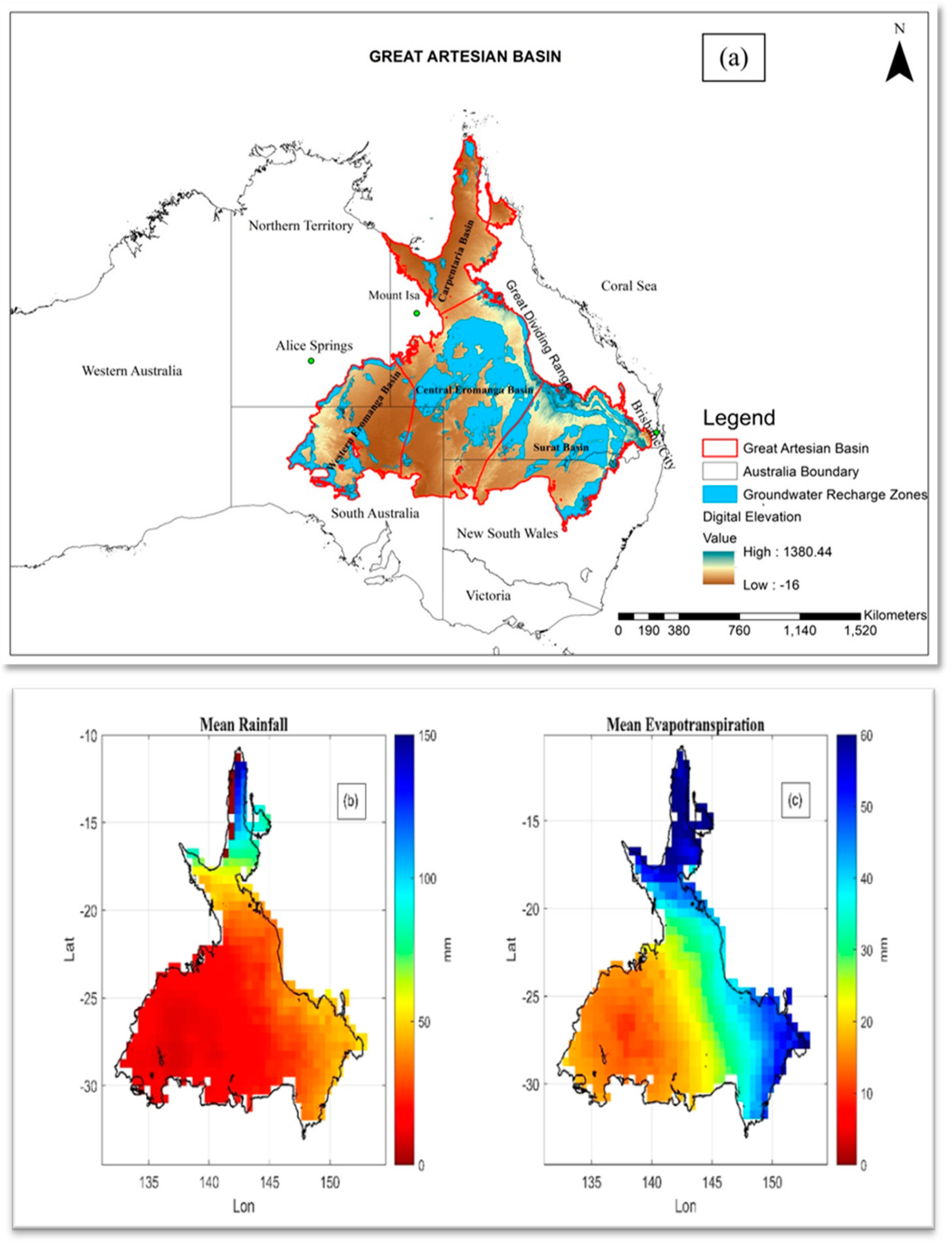
2.1. Study Area and Aquifer Dynamics

The GAB is a continental scale aquifer of approximately 1.7 million square kilometres [40] spread over three states, Queensland, New South Wales, and South Australia, and the Northern Territory [41]. The GAB is comprised of four sub-basins (Figure 1a); Surat, Carpentaria, Central Eromanga, and Western Eromanga [6]. The aquifer system lies in predominantly arid and semi-arid regions [3]. The groundwater temperature in the basin varies between 30° to 100 °C [42]. Groundwater recharge occurs through precipitation in the GAB. Rainfall enters primarily along the uplifted eastern edge of the Great Dividing Range [43,44], with the western edge being a lower recharge zone due to negligible rainfall [45]. It follows that groundwater recharge zones are mostly located in the southeast and central part of the GAB (Figure 1a). Groundwater recharges occur through rainfall and discharge occur through evapotranspiration and extraction from the GAB. Groundwater within the GAB flows in a generally southwest direction, with some of the groundwater moving upward to the surface through various faults and fractures, creating ecologically important springs [46].

Since 1900, the groundwater level in the GAB has decreased [8] due to established mining companies in this area [47]. In addition, climate change (affecting rainfall and aquifer recharge rates) and human activities (e.g., groundwater extraction, mining) over time have an extensive influence on regional aquifer storage, groundwater levels, and surface discharge rates across the GAB [4]. The spatial distribution of average rainfall varies over the GAB between 2002 and 2017 indicates the complex hydrological processes in the GAB (Figure 1b).

The spatial distribution of ET loss (Figure 1c) gives spatial distribution of averaged ET in the GAB system and GLDAS Noah data was used to assess ET between 2002 and 2017. The ET loss is greater in the north and some parts of the southeast region of the GAB.

2.2. Datasets Used

We used four key datasets in this study: (1) terrestrial water storage (TWS) from GRACE satellite, (2) soil moisture storage from GLDAS Noah, (3) rainfall from gridded silos and (4) evapotranspiration from GLDAS Noah. The details of the datasets are outlined in

Table 1. Summary of the datasets used in the study to characterize groundwater storage variations in the GAB.

Data	Source	Temporal Resolution	Spatial Resolution	Period of Study
Terrestrial Water Storage	GRACE	Monthly	0.5° × 0.5°	2002–2017
Soil Moisture Storage	GLDAS NOAH	Monthly	0.25° × 0.25°	2002–2017
Rainfall	Silos Gridded Rainfall	Monthly	0.05° × 0.05°	2002–2017
Evapotranspiration (ET)	GLDAS NOAH	Monthly	0.25° × 0.25°	2002–2017

and Figure 2.

2.3. Gravity Recovery and Climate Experiment (GRACE) Data

In this study, we used terrestrial water storage derived from GRACE-mascons data and covered the period between the years 2002–2017. The data was retrieved from the Center for Space Research (CSR) (http://www2.csr.utexas.edu/grace/RL06_mascons.html, accessed on 15 January 2020) [48] and down sampled to a spatial resolution (0.5° × 0.5°). Hydrological patterns (majorly TWS changes) have been obtained using especially GRACE data in other parts of the world [19,49,50,51].

2.4. Global Land Data Assimilation System (GLDAS) Data

The Global Land Data Assimilation System (GLDAS) generates soil moisture time series and other parameters, such as evapotranspiration, canopy water evaporation, and surface runoff amount, which can improve the understanding of surface water extent [52]. The soil moisture component is an integral part of terrestrial water storage and aids in computing groundwater storage [53]. The GLDAS dataset is a terrestrial modelling system that integrates satellite and ground-based observations. The novelty of this dataset is that it separates the satellite and ground-based observations from the atmosphere [52]. In addition, GLDAS-based soil-moisture data provides an adjustable model time step and output interval and spatial resolution of 1° × 1° [54]. GLDAS soil-moisture dataset (with a spatial resolution of 0.25° × 0.25°) from National Aeronautics and Space Administration (NASA’s) Goddard Space Flight Centre (GSFC) portal (https://disc.gsfc.nasa.gov/datasets/GLDAS_NOAH025_M_2.1/summary?keywords=GLDAS, accessed on 1 April 2020) [55] was used in this study to assess the soil moisture storage component over the GAB from 2002 to 2017.

2.5. Rainfall

We used the silos gridded rainfall data to characterize the spatio-temporal patterns of rainfall in the GAB. The silos dataset (Queensland Government) provides monthly gridded estimates of precipitation in high spatial resolution (0.05° × 0.05°). The monthly rainfall datasets downloaded from the Queensland Government website portal (https://www.longpaddock.qld.gov.au/silo/gridded-data/, accessed on 18 April 2020) [56] were used in this study. In addition, the rainfall data was used to determine its impact on GWS variation.

2.6. Evapotranspiration (ET)

Evapotranspiration is an essential component in water balance estimation over an area [57]. There are various techniques available to assess the ET component for a region [58], and in this study, GLDAS Noah satellite data from the NASA GSFC portal (https://disc.gsfc.nasa.gov/datasets/GLDAS_NOAH025_M_2.1/summary?keywords=Evapotranspiration, accessed on 1 April 2020) [55] was used to extract monthly ET data for the GAB between 2002 and 2017. Further, ET data was used to understand the water loss across the basin and how it affects variation in GWS.

3. Methodology

3.1. Groundwater Storage Variation Estimate from GRACE and GLDAS Satellite Data

GWS variation can be determined from TWS variation (GRACE satellite data) by removing other water storage components (e.g., soil moisture storage and surface water storage) from TWS. For semi-arid regions such as the GAB, the surface water storage component observed in the GRACE TWS data is likely to be negligible, as indicated by the lack of strong gravimetric fluctuation in surface water. Yan et al. [10] concluded that surface water and canopy storage variations contribute only 3% to observed terrestrial water storage over the GAB. If these water storage components are ignored following Yan et al. [10], groundwater storage can be estimated from terrestrial water storage as,

$$\Delta W{S}_{ground}=\Delta TWS-\Delta W{S}_{soil}$$

(1)

where $\Delta W{S}_{ground}$ represents changes in GWS, ∆TWS shows changes in TWS and $\Delta W{S}_{soil}$ represents changes in soil moisture storage. Further, the surface water storage variations are negligible compared to soil moisture and terrestrial water storage variation in Australia [27].

3.2. Spatial-Temporal Patterns of Water Storage Components Using Principal Component Analysis

This study implemented the Principal Component Analysis (PCA) technique on rainfall, TWS and GWS datasets to summarize spatio-temporal variations in rainfall, TWS and GWS. PCA is a statistical decomposition method that decomposes multi-dimensional data and reduces its dimensionality and interpretability [59,60]. The usefulness of this analysis technique has gained popularity in atmospheric science and hydrological science for its dimensionality minimization and simple interpretation nature [61,62,63]. PCA transforms the dataset (e.g., TWS, GWS and rainfall) linearly and obtains a set of orthogonal vectors encompassing the very same region [60,64]. Mathematically, the eigenvalues and eigenvectors of a covariance matrix determine the principal components (PCs) of a given dataset [65]. This method helped in determining principal components (i.e., temporal variations) and empirical orthogonal functions (EOFs) (i.e., spatial maps). A scree plot analysis was employed to ensure that only significant orthogonal modes of variability were interpreted in all the hydrological units such as TWS, GWS and rainfall over the GAB [61]. The following equation was used to decompose variations in rainfall, TWS and GWS,

$$X\left(t\right)= {\displaystyle \sum }_{k=1}^n{a}_{\left(k\right)}{p}_k,$$

(2)

where a_(k) (t) represents temporal variations (also known as standardized scores) and p_k are the corresponding spatial patterns (known as the empirical orthogonal functions [EOF]-loadings). The standardized score is part of the total variation proportional to the total covariance in the time described by the eigenvector (EOF). EOFs have been normalized using the standard deviation of their corresponding principal components. For instance, while the EOF represents the spatial distribution of TWS, GWS or rainfall, the EOF/PC pairs are called PCA modes. In our study, PCA was employed to statistically decompose GRACE and rainfall datasets into PCs (temporal) and EOFs (spatial) to help in identifying the dominant patterns of GWS, TWS and rainfall in the GAB. Across the entire space-time dataset, 20 out of 183 months (10.9%) of total observations were missing over the 2002–2017 study period. These missing values occurred as random gaps in between years and were filled using linear interpolation, which is a common method to reconstruct or predict missing hydrological time series of this nature [27,59]. This interpolation did not impact on the overall data quality. With a consecutive monthly time-series of GRACE observations (183 time-steps starting from April 2002–June 2017) following the linear interpolation, we then implemented the PCA.

3.3. Time Series Analyses of Water Storage Components

Time series analysis of monthly averaged water storage components (TWS, GWS, ET and rainfall) was performed to determine the changes in these hydrological fluxes in time. In addition, time-series analyses were also executed to understand the variation and connectivity in different water storage components at each sub-basin (Carpentaria, Surat, Western Eromanga, and Central Eromanga) and for the entire GAB.

3.4. Average Annual Cycle and Deseasonalization of GWS and Rainfall

The average annual cycles of GWS and rainfall for each sub-basin in the GAB were assessed to investigate seasonal variation in GWS and rainfall. GWS variation and rainfall amplitudes were observed to find the peaks for respective months and helpful in finding the phase lag between rainfall and GWS variation. In addition to assessing the average annual cycles, deseasonalization of GWS and rainfall time series was undertaken to assess the human footprints and climatic contributions to the basin’s hydrology. Here, deseasonalizing means eliminating the annual seasonal signals from the GWS and rainfall time series.

To further understand the drivers of GWS variation across the basin, the GWS-rainfall relationship was analyzed using least square method. To this end, the spatial patterns of GWS variation and rainfall trends [66] between different time periods such as 2002–2008, 2009–2012 and then from 2012–2017 were executed using least square analysis.

3.5. Relationship between Water Storage Components (TWS, GWS, ET) and Rainfall Using Cross-Correlation Analyses

To further understand how the GWS varied in response to climate and non-climatic factors, cross-correlation analysis was used to evaluate the strength of agreement between rainfall, ET, and the water storage components TWS and GWS [59,61]. By implementing cross-correlation method on various water storage components such as rainfall, ET, GWS and TWS, the GAB sub-basins with maximum correlation can be obtained (i.e., between rainfall and GWS, rainfall and TWS, ET and GWS), to observe the GWS-rainfall relationship and lag months corresponding to the maximum correlation. The time-lagged correlation between the water storage components (e.g., GWS variation and rainfall) helped understand the response time (i.e., time taken by groundwater storage to recharge from rainfall). Spatio-temporal variations in groundwater storage relating to rainfall provided insight into climate variability and human intervention impacts in the GAB, as reported by some past studies [3,4,5,10,35,37,38,39].

3.6. Understanding GWS Changes-Rainfall Relationship Using Multi-Linear Regression Analysis

Multiple linear regression was used to model the trend, annual and semi-annual components of variation in GWS and rainfall. Mathematically, it can be represented [18,59] as,

$$\mathrm{X}\left(\mathrm{t}\right) =\beta 0+\beta 1t+\beta 2\sin \left(2\pi t\right)+\beta 3\cos \left(2\pi t\right)+\beta 4\sin 2\pi t+\beta 5\cos \left(2\pi t\right)+\beta 6E\left(t+\phi E\right)+\epsilon$$

(3)

where X(t) represents GWS or precipitation at time t, β0 represents constant, β1 shows linear trend, β2 and β3 shows periodic components (annual signal), while β4 and β5 show periodic components (semi-annual signals). The term β6 is the amplitude of GWS variation linked to climate signals. The variable E represents the normalized sequence of respective climate index (i.e., after eliminating long-term average) and $\phi$E shows the phase difference between GWS temporal variation and respective climate mode. ε is the error and shows the deviation between model outputs and observations. To validate the strength of MLRA, other parameters such as root mean square error (RMSE) and coefficient of determination (R²) were assessed grid by grid. Using the multi-linear regression analysis (MLRA), trends and harmonic components of GWS changes such as rainfall patterns over the GAB areas were obtained [61,67]. This approach helps in assessing the GAB region in a more accurate way using RMSE and R² parameters.

4. Results

4.1. Spatial and Temporal Changes in Rainfall across the GAB

The gridded rainfall data over the GAB for a 15-year window (i.e., 2002–2017) is analyzed using PCA. The mean monthly gridded rainfall pattern observed from rainfall data ranges from 5 to 180 mm with higher-level over the northern (i.e., in Carpentaria sub-basin) part and lesser over the western (Western Eromanga sub-basin) GAB (Figure 1b). The mean distribution of rainfall over GAB shows that much of it falls in the northern region compared with the typically dry southwest region of the basin (Figure 1b).

The total variability in rainfall observed by the first three principal component (PC) modes is 78.67% (Figure 3). In the first principal component, EOF loadings (or spatial patterns) are relatively strong and account for 63% of the cumulative variability in rainfall and are majorly localized over the Northern (Carpentaria sub-basin) part of the GAB (Figure 3a). TWS variations in the first principal mode are also localized in the northern region (Carpentaria), suggesting rainfall as a driver of water storage in the region. The second mode (Figure 3b) represents 9.81% of the cumulative variability. Figure 3b shows semi-annual rainfall distribution concentrated over the northern (Carpentaria sub-basin) part of the GAB. The third PC mode (Figure 3c) accounts for approximately 6% of the cumulative variability. The temporal patterns of rainfall associated with the spatial loadings (spatial patterns) in the northern region show strong annual variability (PC-1/EOF-1, Figure 3d), contrasting the multi-annual and seasonal variations observed in PCs 2 and 3 (Figure 3e,f).

4.2. Spatio-Temporal Patterns of Water Storage Components in GAB

4.2.1. GRACE-Derived Terrestrial Water Storage

Changes in terrestrial water storage is analyzed using the PCA technique. From the scree plot analysis of terrestrial water storage (TWS), the first three PC modes accounted for 92.75% of the total variance and are chosen as the dominant patterns (or leading modes) of variability in GRACE hydrological signals over the GAB. The first PC mode (Figure 4a,d) of TWS shows relatively stronger spatial (EOF loadings) and temporal patterns in the northern region (Carpentaria sub-basin). Other orthogonal modes of variations in TWS (Figure 4b,c) show multi-annual variations (PC-2) and short-term GRACE-hydrological signals (PC-3) and accounts for the remaining variability (28.79% and 3.26%, for the second and third modes, respectively). The GRACE-hydrological signals in these modes are associated with parts of Surat and Western Eromanga sub-basins (Figure 4b,c). As with temporal evolutions of TWS in the Carpentaria sub-basin, they both show pronounced peak amplitudes between 2010 and 2012 (Figure 4d–f). When the temporal and spatial patterns are jointly interpreted, changes in TWS show declines in the temporal series associated with parts of the Surat sub-basin since 2012 (Figure 4e). Looking closely at the Carpentaria sub-basin, a similar trend is noticeable but is gradual (Figure 4b).

4.2.2. Changes in Groundwater Storage

The spatio-temporal patterns in the first PC mode for groundwater storage variation reveal annual groundwater storage localized over the northern region of the basin. This is the dominant pattern of GWS accounting for approximately 59% of the total variability in the basin (Figure 5a,d). The second PC mode captures about 21% of the total variability in GWS and depicts relatively higher multiannual variation in the southeast region of GAB (Figure 5b). The corresponding temporal series (Figure 5e) associated with this spatial pattern shows peak amplitudes that coincide with the ‘big wet period’ and a steady decline after this period (2013–2017). Figure 5c,f show a 7.11% total variability in the third PC mode and represents the multi-annual variations over the GAB. In this mode, the north and southwest part (i.e., in Carpentaria and Western Eromanga sub-basin) of the GAB depicts higher EOF loadings.

4.3. Temporal Variations of Water Storage Components in GAB

The temporal variations in different water storage components (GWS, TWS, ET and rainfall) over GAB and its sub-basins during the 15-year period (2002–2017) are analyzed, and they exhibit remarkable fluctuations (Figure 6). GWS anomalies over the GAB have experienced three main decreasing periods (2005–2006, 2008–2009 and 2015–2016) and one significant increasing period between 2010 and 2012. Increased TWS between 2009 and 2011 coincided with a rise in GWS variation (Figure 6a). TWS and GWS variation obtained for the Carpentaria sub-basin show similarity with each other in terms of magnitude and time. However, there is some delay between GWS variation and rainfall (Figure 6b), which is discussed later in the manuscript. For the Surat sub-basin, water budget indicators (TWS, GWS, rainfall and ET) show temporal variations that suggest they are related to one another such that rainfall acts as a key input to the hydrological system and results in a consistent response of TWS followed by GWS (Figure 6c). Considering the Central Eromanga sub-basin, the variation in water storage also shows higher amplitude between 2010 and 2012 (Figure 6d), as observed for the Surat sub-basin (Figure 6c). GWS variation results for different GAB sub-basins and the whole of the GAB strongly represent the complexity of hydrological processes within the GAB. The fluctuations in rainfall in the Surat sub-basin, for instance, appear to be in the opposite phase with GWS, in contrast with the Carpentaria, where the temporal evolutions (patterns) of both data maintain the same phase, largely due to similar annual cycles. The Eromanga sub-basins (central and west) are typically dry, and the response of groundwater to periods with pronounced strong peak in annual rainfall (e.g., 2004, 2007, 2008/2009, for the Central Eromanga) are inconsistent and in the opposite phase (Figure 6d,e).

4.4. Average Annual Cycles and Deseasonalization of GWS and Rainfall

Looking at the individual sub-basin responses, apart from the Carpentaria (Figure 7a), the seasonal annual cycles of GWS are in opposite phase with rainfall (Figure 7c,e,g). Deseasonalized GWS and rainfall time series are evident when annual seasonal cycles were removed from GWS signals. To track human footprints/factors other than rainfall in GWS variation, the long-term trend and seasonal signals are observed and GWS variation time-series with non-climatic factors is obtained. Here, long-term trend provides information on what influences water storage between 2002 and 2017 during water years (e.g., flood or other natural variability occurrence). From this, it can be deduced that an increase in rainfall will likely cause an increase in TWS or GWS and the lack of rainfall can cause a decline in GWS. It is likely that this increase or decrease in GWS is climate-induced (Figure 7b,d,f,h). However, GWS usage during the March-November period, when rainfall is largely limited, may have an impact on GWS variations (seasonal signal or human footprints). Isolation of GWS seasonal cycles from its averaged times-series can help in finding the inclusion of human-induced factors in GWS variation (Figure 7b,d,f,h). There are significant differences between non-deseasonalized and deseasonalized GWS signals for some of the sub-basins (indicated by the red color) where it is possible to tease apart some factors that are driving the GWS variation in the basin (Figure 7b,d,f,h).

Observing the deseasonalized GWS time series for the Carpentaria, rainfall is strongly associated with GWS variation (Figure 7a). In other sub-basins, deseasonalized GWS time series shows that GWS variation is associated with factors other than rainfall (Figure 7d,f,h). Western Eromanga, an arid region in the GAB (Figure 1b), shows the existence of other non-climatic factors associated with varying GWS (Figure 7h). However, there is significant difference between non-deseasonalized and deseasonalized GWS time series in the Surat and Central Eromanga sub-basins depicting that GWS variation in these regions are likely driven by the influence of climatic and non-climatic factors (e.g., human extraction, industrial and agricultural use), especially in the Surat sub-basin (Figure 7d,f).

Isolating GWS seasonal cycles from the averaged GWS time series showed that GWS variation in the Carpentaria sub-basin has a strong GWS annual component and is largely driven by annual rainfall (Figure 7b). The Surat, Central Eromanga and Western Eromanga sub-basins show multi-seasonal oscillations that capture extreme events such as the big wet period during 2010–2012 period (Figure 7d,f,h). Regarding Figure 7d,f,h, it seems the declines during the 2012–2016 period appears to be sharper in the deseasonalized GWS. Overall, the steady declining trends resulting from a probable human groundwater use are evident in these regions and appear to be more pronounced during the post big wet period.

4.5. Trends in Ground Water Storage Variations

The spatial patterns of trends in GWS and rainfall over GAB reflect a complexity of geology and hydrological processes in the basin. We found that long-term GWS variation over the southeast region is inconsistent with rainfall variation (Figure 8a,e). The PCA results of GWS (Figure 5b,e) highlight the same signals and validate the PCA method in understanding the spatial and temporal distribution of changes in water storage components. Along with this, the short term GWS trend analyses (2002–2009 and 2012–2017) exhibit completely different patterns in relation to rainfall. For instance, GWS varies linearly at rate of −5 mm/year while rainfall linear rate is 4 mm/year during 2002–2008 period (Figure 8b,f). Similarly, GWS varies linearly at a rate of up to −20 mm/year while rainfall varies linearly at a rate of 5 mm/year during 2012–2017 period. These dissimilarities exist over southeast region (Figure 8b,f,d,h) except for a short period, January 2009–March 2012, in which GWS trend analyses broadly coincide with the rainfall trends (Figure 8c,g). It is likely that GWS in some GAB areas, such as the northern region (Figure 8a,c–e,g,h), are driven by climate variation.

4.6. Response of Land Water Storage to Climate Variability

Rainfall and evapotranspiration are major factors causing GWS variations [11]. For that reason, the response of TWS and GWS to rainfall and ET is assessed. Figure 9 represents the maximum correlation coefficients (r) value between the two variables (for example, GWS and rainfall) and the lags at which GWS and rainfall show maximum correlation (Figure 9a,b). From the observed r value, it is clear that rainfall drives GWS variation for more than 50% of the GAB. For example, GWS variation shows a relatively high correlation with rainfall in the northern and southeast regions of the GAB (Figure 9). This is also confirmed from the deseasonalized trends in the Carpentaria sub-basin (Figure 7a,b). The north and southeast parts of the GAB show that rainfall precedes GWS variation (lags ranging from approximately 2–12 months) with correlation coefficients ranging from 0.50 to 0.70 (Figure 9a,b). As can be seen from Figure 9b, different regions in GAB show different lag time. Apart from some locations with a lag time of approximately 12 months between rainfall and GWS, in the southeast and north regions rainfall precedes GWS variation by 2–5 months in much of the locations where correlations are greater than 0.50 (Figure 9b).

There are some parts of the GAB, such as the southwest region, that are characterized by small rainfall amounts. The correlation between rainfall and GWS variation in the southwest region is lower than other regions, ranging from 0.20 to 0.30 (Figure 9a). The southwest region’s rainfall is lagging behind GWS variation with a phase of approximately more than a year (Figure 9b). This is expected as the southwest region is characterized by a dry climate [5]. Relatively low values of correlation coefficients (r) are observed for the southwest region of between 0.10 and 0.30. Low values of r could imply weaker influence of rainfall over groundwater recharge. Overall, rainfall drives the hydrology (i.e., GWS, TWS) in the northern region (Figure 9a,c). Deseasonalized and average annual cycles of GWS and rainfall also validate these results for each of the sub-basin (Figure 7).

Rainfall has a strong association with variation in TWS over more than half of the GAB (Figure 9c). Rainfall commonly precedes TWS variations by 2–3 months and is consistent in the GAB except for the southwest region where rainfall is considerably limited (Figure 9d). A strong correlation exists between ET and GWS variation for most of the GAB except for some of the southwest regions (Figure 9e). The north and southeast regions of the GAB show a negative phase lag in 2 to 5 months between ET and GWS variation (ET leads GWS variation). The southwest regions show a positive phase lag between GWS variation and ET (GWS variation precedes ET) of 15 months (Figure 9f). This is consistent with the observed relationship between GWS variation and rainfall for the southwest region of the GAB (Figure 9a).

4.7. Understanding Drivers of Groundwater Variability

Multiple linear regression analysis (MLRA) is implemented to understand drivers of variations in GWS across the GAB. GWS and rainfall indicates consistency in average annual amplitudes (Figure 10a,f) and also coincides with the leading orthogonal modes of variability in both data (Figure 3 and Figure 5). However, GWS in the north of Eromanga shows an annual signal (Figure 10a,b). GWS trends indicate complete dissimilarity with the spatial patterns of rainfall trends for Central and Western Eromanga sub-basins (Figure 10b,c,g,h). In contrast with rainfall, the only sub-basin where significant trend in GWS exist is the Surat sub-basin (Figure 10g,h). The disparity in GWS and rainfall trends (Figure 10c,h) observed in the Surat sub-basin possibly reflects the complexity of geology and climate across the GAB [3]. Root mean square error (RMSE) values in the southern regions (arid/semi-arid region) of the basin are low for GWS and rainfall and relatively higher in the northern regions (Figure 10d,i). Values of R² (i.e., GWS) ranging from 0.80 to 1.00 are observed over the northern region of basin (Figure 10e). Such higher values of R² indicate that GWS variation in the northern part of GAB basin is likely affected by rainfall.

5. Discussion

5.1. Changes in Terrestrial Water Storage

TWS is an indicator of freshwater availability and plays a vital role in quantifying important hydrological changes [68,69]. The temporal variation of TWS and GWS indicate that the GAB and its sub-basins have experienced increases in TWS variation between 2009 and 2011 (Figure 6). A strong La Niña occurred between 2010 and 2012 [70], causing flooding in the northeast and southeast regions of Queensland. This climatic event was likely responsible for increases in terrestrial water storage between 2010 and 2012 in the northeast and southeast regions of the GAB [70], suggesting rainfall to be a substantial driver of variation in TWS.

TWS variation in the GAB was largely related to climate factors such as rainfall and evapotranspiration. Rainfall and evapotranspiration values were high in the north and southeast regions of the GAB compared with the southwest region where they are relatively lower. Furthermore, cross-correlation between TWS and rainfall were high in the north and southeast regions and imply rainfall to be a significant factor behind variations in TWS for these regions. ET may also cause variation in TWS. As an outgoing flux and water budget indicator, ET can serve as a sink term that induces strong changes in hydrological conditions apart from rainfall. Given the semi-arid nature of the south-east region (Surat sub-basin), and the considerably strong correlations between GWS and rainfall, ET is likely to be crucial to the water balance of this region. All-in-all, the influence of ET on GWS is likely to be much greater in parts of the GAB where rainfall is low and ET is high.

5.2. Understanding Changes in Groundwater Storage over the GAB

Our study presents the spatiotemporal patterns of rainfall in the GAB and evaluates its impact on hydrological stores (TWS and groundwater). We observed that rainfall has a leading role in driving GWS variation in the northern region of GAB, and other non-climatic factors (e.g., human water extraction) have also been recognized as driving GWS changes in south regions of the GAB, especially southeast (Surat sub-basin) [35,39]. Factors causing variation in GWS may decrease the number of springs and impact groundwater-dependent ecosystems.

The GAB is a complex hydrological basin. Based on our deseasonalized GWS and rainfall results, GWS variation in the southeast (Surat) region and the northern (Carpentaria) region showed that climate conditions and likely other factors, such as anthropogenic groundwater extraction, are associated with changes in GWS (Figure 7). GWS variation, rainfall trends and the cross-correlation results confirm the observations made from deseasonalized GWS and rainfall patterns (Figure 8 and Figure 9). The inconsistencies that we observed in RMSE values across the southeast region (Figure 10d,j) may be due to inter-annual changes in rainfall or the complex hydro-geology in the basin [71]. Low values of R² (coefficient of determination) over the southern region could suggest non-climatic influence or human intervention for these parts of the basin (Figure 10e,j) [61]. This is supported by the MLRA results for rainfall and GWS variation, which suggest influence of human use on GWS variation. For instance, pastoral industries, coal, and gas power generation plants exist in the Surat sub-basin and depend on groundwater resources [72]. These groundwater extractions consequently impact groundwater storage in the basin. Kent et al. [38] exhaustively analyzed the water extraction in the southeast GAB from 1900 to 2015 and helped finding the temporal patterns of groundwater decline in the region.

GWS variation showed negative trends in the 2005–2006 and 2008–2009 periods before a La Niña [70] event which caused widespread flooding in the northeast and southeast regions of Queensland in 2011 (Figure 6). The sharp rise in GWS over this period is likely linked to this strong La Niña event (Figure 5a). High rainfall was associated with a sharp rise in GWS after 2009 (Figure 5d). Given this, rainfall is most likely an essential contributor to recharging groundwater storage. The cross-correlation results between GWS variation and rainfall (r = 0.5–0.7) highlight that rainfall is a main factor behind varying GWS for more than half of the GAB where rainfall precedes GWS variation by two to four months (Figure 9a,b).

We observed a relative temporal difference between TWS and GWS variations. There is a noticeable water loss factor (e.g., evapotranspiration) creating a relative difference between GWS and TWS variation. To understand the changes of TWS, ET over the GAB was evaluated between 2002 and 2017. Additionally, the GWS variation and ET were cross-correlated with each other (Figure 9e,f). MLRA results of rainfall and GWS confirm the results obtained by cross-correlation analysis and suggest that GWS variation is driven by climatic variability over tropical parts of the GAB (i.e., Carpentaria) and by the combination of climatic and non-climatic factors over arid and semi-arid GAB (i.e., Western Eromanga, Surat and Central Eromanga).

Changing climate conditions impact the world in terms of increased or decreased level of rainfall, water storage, water inundation and drought [27,73,74,75,76,77,78]. In past years, research on the GAB has highlighted that varying climatic conditions and unsustainable use of groundwater (e.g., through boreholes) has likely resulted in the decline of groundwater stores and impacted sensitive ecosystems [6,8,10]. The water storage in semi-arid or arid regions largely depends on rainfall [79,80,81]. GWS variations in the basins are likely caused by climate conditions and events such as ENSO (El Nino Southern Oscillation) [82,83]. The GWS variation in the GAB is influenced by changes in annual and seasonal rainfall in the GAB. Recent studies observed a strong relationship between climate conditions and water storage variation [5,10]. Thus, quantifying climate variability factors such as rainfall effects on GWS variation across the GAB could be advantageous for groundwater management strategies by finding the locations with strong effects of rainfall on GWS and the locations deprived of rainfall.

We can better manage groundwater-dependent ecosystems once we have a better understanding of groundwater storage variation in the GAB. Springs are groundwater-dependent ecosystems and are a permanent water source that sustains wildlife and habitat including endemic vegetation and fauna [84]. However, pastoral and mining activities may have adverse impacts on many springs, as observed in southeast regions of the GAB [2]. Identifying groundwater storage variation hotspots help us understand how climate effects and human impact vary spatially and temporally across the GAB and is necessary for the better management of groundwater-dependent ecosystems including springs [85].

6. Conclusions

The main conclusions of the study are outlined below:

a.

GWS varied most in Carpentaria sub-basin and some parts of the Surat sub-basin. The relatively high amount of rainfall within the Carpentaria and south-east region of the Surat sub-basin is the main factor driving the observed variability in GWS in these regions. Multi-annual variations in GWS are prominent in the Surat sub-basin and coincide with variation in rainfall. This amplification of GWS variation is observed as a result of changing climate conditions and potentially human water extraction in the Surat sub-basin.

b.

GWS variation over the GAB between January 2009 and March 2012 period shows the Surat sub-basin had positive and strongest rise (40 mm/year) in GWS coinciding with a wet period following the Millennium drought. However, the Surat sub-basin showed negative trends before and after the 2009–2012 period. Overall, rainfall and GWS variation trends are consistent for the Carpentaria sub-basin and inconsistent for south regions of GAB, which indicates that other important drivers of variation in GWS exist apart from rainfall.

c.

In general, the rainfall-GWS variation relationship indicates a time lag of two to three months for more than half of the GAB. The GWS-rainfall relationship is strong for more than half of the GAB; however, it is low for some parts of GAB (e.g., Western Eromanga and some parts of Surat sub-basin). Such regions show a phase lag of approximately 12 months and highlight the probable effects of non-climate factors on GWS variation in addition to climatic variation.

d.

The ET correlates more with GWS variation than the rainfall in the Surat sub-basin (Figure 9a,e). This observation indicates that ET is an important factor in the recharge processes in this low rainfall region (Figure 1b). If rainfall declines in this region, then it could be a problem for recharge in the Surat sub-basin.

e.

GWS variation in the southern regions of GAB (i.e., in Surat, Western Eromanga and Central Eromanga sub-basins) showed a weaker relationship with climate (i.e., rainfall). This relationship could potentially be due to the combined effects of human water extraction and complex hydro-geological processes.

References

1. Hillier, J.R.; Foster, L. The Great Artesian Basin—Is There a Sustainable Yield. In Proceedings of the International Association of Hydrologists Conference, Darwin, Australia, 12–17 May 2002. [Google Scholar]
2. Fensham, R.; Ponder, W.; Fairfax, R. Recovery Plan for the Community of Native Species Dependent on Natural Discharge of Groundwater from the Great Artesian Basin; Report to Department of the Environment, Water, Heritage and the Arts; Department of Envrionment and Resource Management: Canberra, Australia, 2010. [Google Scholar]
3. Habermehl, M.A. The Great Artesian Basin, Australia. In Non-Renewable Groundwater Resources: A Guidebook on Socially-Sustainable Management for Water-Policy Makers; Foster, S., Loucks, D.P., Eds.; UNESCO: Paris, France, 2006; pp. 82–88. [Google Scholar]
4. Welsh, W.; Moore, C.; Turnadge, C.; Smith, A.; Barr, A. Modelling of Climate and Groundwater Development a Technical Report to the Australian Government from the CSIRO Great Artesian Basin Water Resource Assessment; CSIRO Water for a Healthy Country Flagship: Canberra, Australia, 2012. [Google Scholar]
5. Fu, G.; Zou, Y.; Crosbie, R.S.; Barron, O. Climate changes and variability in the Great Artesian Basin (Australia), future projections, and implications for groundwater management. Hydrogeol. J. 2020, 28, 375–391. [Google Scholar] [CrossRef]
6. Habermehl, M.A. The evolving understanding of the Great Artesian Basin (Australia), from discovery to current hydrogeological interpretations. Hydrogeol. J. 2019, 28, 13–36. [Google Scholar] [CrossRef]
7. Powell, O.; Silcock, J.; Fensham, R. Oases to Oblivion: The Rapid Demise of Springs in the South-Eastern Great Artesian Basin, Australia. Ground Water 2013, 53, 171–178. [Google Scholar] [CrossRef]
8. Smerdon, B.D.; Marston, F.M.; Ransley, T.R. Water Resource Assessment for the Great Artesian Basin Synthesis of a Report to the Australian Government from the CSIRO Great Artesian Basin Water Resource Assessment; CSIRO Water for a Healthy Country Flagship: Canberra, Australia, 2012. [Google Scholar]
9. Zhou, Y.; Li, W. A review of regional groundwater flow modeling. Geosci. Front. 2011, 2, 205–214. [Google Scholar] [CrossRef] [Green Version]
10. Yan, J.; Jia, S.; Lv, A.; Mahmood, R.; Zhu, W. locysis of the spatio-temporal variability of terrestrial water storage in the Great Artesian Basin, Australia. Water Sci. Technol. Water Supply 2016, 17, 324–341. [Google Scholar] [CrossRef]
11. Wu, W.-Y.; Lo, M.-H.; Wada, Y.; Famiglietti, J.S.; Reager, J.T.; Yeh, P.J.-F.; Ducharne, A.; Yang, Z.-L. Divergent effects of climate change on future groundwater availability in key mid-latitude aquifers. Nat. Commun. 2020, 11, 1–9. [Google Scholar] [CrossRef]
12. Xie, Z.; Huete, A.; Restrepo-Coupe, N.; Ma, X.; Devadas, R.; Caprarelli, G. Spatial partitioning and temporal evolution of Australia’s total water storage under extreme hydroclimatic impacts. Remote Sens. Environ. 2016, 183, 43–52. [Google Scholar] [CrossRef]
13. Tangdamrongsub, N.; Ditmar, P.G.; Steele-Dunne, S.C.; Gunter, B.C.; Sutanudjaja, E.H. Assessing total water storage and identifying flood events over Tonlé Sap basin in Cambodia using GRACE and MODIS satellite observations combined with hydrological models. Remote Sens. Environ. 2016, 181, 162–173. [Google Scholar] [CrossRef] [Green Version]
14. Zhang, Z.; Chao, B.F.; Chen, J.; Wilson, C.R. Terrestrial water storage anomalies of Yangtze River Basin droughts observed by GRACE and connections with ENSO. Glob. Planet. Chang. 2015, 126, 35–45. [Google Scholar] [CrossRef]
15. Thomas, A.C.; Reager, J.T.; Famiglietti, J.S.; Rodell, M. A GRACE-based water storage deficit approach for hydrological drought characterization. Geophys. Res. Lett. 2014, 41, 1537–1545. [Google Scholar] [CrossRef] [Green Version]
16. Van Dijk, A.I.J.M.; Renzullo, L.J.; Rodell, M. Use of Gravity Recovery and Climate Experiment terrestrial water storage retrievals to evaluate model estimates by the Australian water resources assessment system. Water Resour. Res. 2011, 47, W11524. [Google Scholar] [CrossRef]
17. Brunner, P.; Franssen, H.-J.H.; Kgotlhang, L.; Bauer-Gottwein, P.; Kinzelbach, W. How can remote sensing contribute in groundwater modeling? Hydrogeol. J. 2007, 15, 5–18. [Google Scholar] [CrossRef] [Green Version]
18. Thomas, B.F.; Famiglietti, J.S. Identifying Climate-Induced Groundwater Depletion in GRACE Observations. Sci. Rep. 2019, 9, 4124. [Google Scholar] [CrossRef] [Green Version]
19. Watkins, M.M.; Wiese, D.N.; Yuan, D.-N.; Boening, C.; Landerer, F.W. Improved methods for observing Earth’s time variable mass distribution with GRACE using spherical cap mascons. J. Geophys. Res. Solid Earth 2015, 120, 2648–2671. [Google Scholar] [CrossRef]
20. Tapley, B.D.; Bettadpur, S.; Ries, J.C.; Thompson, P.F.; Watkins, M.M. GRACE Measurements of Mass Variability in the Earth System. Science 2004, 305, 503–505. [Google Scholar] [CrossRef] [PubMed] [Green Version]
21. Frappart, F.; Ramillien, G. Monitoring Groundwater Storage Changes Using the Gravity Recovery and Climate Experiment (GRACE) Satellite Mission: A Review. Remote Sens. 2018, 10, 829. [Google Scholar] [CrossRef] [Green Version]
22. Bhanja, S.N.; Mukherjee, A.; Rodell, M.; Wada, Y.; Chattopadhyay, S.; Velicogna, I.; Pangaluru, K.; Famiglietti, J.S. Groundwater rejuvenation in parts of India influenced by water-policy change implementation. Sci. Rep. 2017, 7, 7453. [Google Scholar] [CrossRef] [Green Version]
23. Richey, A.S.; Thomas, B.F.; Lo, M.; Reager, J.T.; Famiglietti, J.S.; Voss, K.; Swenson, S.; Rodell, M. Quantifying renewable groundwater stress with GRACE. Water Resour. Res. 2015, 51, 5217–5238. [Google Scholar] [CrossRef]
24. Scanlon, B.R.; Zhang, Z.; Reedy, R.C.; Pool, D.R.; Save, H.; Long, D.; Chen, J.; Wolock, D.M.; Conway, B.D.; Winester, D. Hydrologic implications of GRACE satellite data in the Colorado River Basin. Water Resour. Res. 2015, 51, 9891–9903. [Google Scholar] [CrossRef]
25. Voss, K.A.; Famiglietti, J.S.; Lo, M.-H.; De Linage, C.; Rodell, M.; Swenson, S.C. Groundwater depletion in the Middle East from GRACE with implications for transboundary water management in the Tigris-Euphrates-Western Iran region. Water Resour. Res. 2013, 49, 904–914. [Google Scholar] [CrossRef] [Green Version]
26. Moiwo, J.P.; Yang, Y.; Tao, F.; Lu, W.; Han, S. Water storage change in the Himalayas from the Gravity Recovery and Climate Experiment (GRACE) and an empirical climate model. Water Resour. Res. 2011, 47, 1–13. [Google Scholar] [CrossRef] [Green Version]
27. Ndehedehe, C.E.; Ferreira, V.G.; Agutu, N.O.; Onojeghuo, A.O.; Okwuashi, O.; Kassahun, H.T.; Dewan, A. What if the rains do not come? J. Hydrol. 2021, 595, 126040. [Google Scholar] [CrossRef]
28. Chen, H.; Zhang, W.; Nie, N.; Guo, Y. Long-term groundwater storage variations estimated in the Songhua River Basin by using GRACE products, land surface models, and in-situ observations. Sci. Total Environ. 2019, 649, 372–387. [Google Scholar] [CrossRef] [PubMed]
29. Rodell, M.; Famiglietti, J.S.; Wiese, D.N.; Reager, J.T.; Beaudoing, H.K.; Landerer, F.W.; Lo, M.-H. Emerging trends in global freshwater availability. Nature 2018, 557, 651–659. [Google Scholar] [CrossRef]
30. Ojha, C.; Shirzaei, M.; Werth, S.; Argus, D.F.; Farr, T.G. Sustained Groundwater Loss in California’s Central Valley Exacerbated by Intense Drought Periods. Water Resour. Res. 2018, 54, 4449–4460. [Google Scholar] [CrossRef]
31. Nigatu, Z.M.; Fan, D.; You, W. GRACE products and land surface models for estimating the changes in key water storage components in the Nile River Basin. Adv. Space Res. 2021, 67, 1896–1913. [Google Scholar] [CrossRef]
32. Shamsudduha, M.; Taylor, R.G. Groundwater storage dynamics in the world’s large aquifer systems from GRACE: Uncertainty and role of extreme precipitation. Earth Syst. Dyn. 2020, 11, 755–774. [Google Scholar] [CrossRef]
33. Opie, S.; Taylor, R.G.; Brierley, C.M.; Shamsudduha, M.; Cuthbert, M.O. Climate–groundwater dynamics inferred from GRACE and the role of hydraulic memory. Earth Syst. Dyn. 2020, 11, 775–791. [Google Scholar] [CrossRef]
34. Ndehedehe, C.E.; Agutu, N.O.; Okwuashi, O.; Ferreira, V. Spatio-temporal variability of droughts and terrestrial water storage over Lake Chad Basin using independent component analysis. J. Hydrol. 2016, 540, 106–128. [Google Scholar] [CrossRef] [Green Version]
35. Singh, D.; Flook, S.; Pandey, S.; Erasmus, D.; Foster, L.; Phillipson, K.; Lowry, S. Improved characterisation of unmetered stock and domestic groundwater use in the Surat and Southern Bowen basins of the Great Artesian Basin (Australia). Hydrogeol. J. 2020, 28, 413–426. [Google Scholar] [CrossRef]
36. Radke, B.M.; Ferguson, J.; Cresswell, R.G.; Ransley, T.R.; Habermehl, M.A. Hydrochemistry and Implied Hydrodynamics of the Cadna-Owie—Hooray Aquifer, Great Artesian Basin; Radke, B.M., Ferguson, J., Cresswell, R.G., Ransley, T.R., Habermehl, M.A., Eds.; Bureau of Rural Sciences: Canberra, Australia, 2000; Available online: http://hdl.handle.net/102.100.100/210084?index=1 (accessed on 15 January 2020).
37. Robertson, J. Challenges in sustainably managing groundwater in the Australian Great Artesian Basin: Lessons from current and historic legislative regimes. Hydrogeol. J. 2019, 28, 343–360. [Google Scholar] [CrossRef] [Green Version]
38. Kent, C.R.; Pandey, S.; Turner, N.; Dickinson, C.G.; Jamieson, M. Estimating current and historical groundwater abstraction from the Great Artesian Basin and other regional-scale aquifers in Queensland, Australia. Hydrogeol. J. 2019, 28, 393–412. [Google Scholar] [CrossRef] [Green Version]
39. Jamieson, M.; Elson, M.; Carruthers, R.; Ordens, C.M. The contribution of citizen science in managing and monitoring groundwater systems impacted by coal seam gas production: An example from the Surat Basin in Australia’s Great Artesian Basin. Hydrogeol. J. 2019, 28, 439–459. [Google Scholar] [CrossRef] [Green Version]
40. Great Artesian Basin Consultative Council (GABCC). Great Artesian Basin Resource Study; Cox, R., Barron, A., Eds.; Great Artesian Basin Consultative Council: Brisbane, Australia, 1998; p. 235. [Google Scholar]
41. Herczeg, A.L.; Love, A.J. Review of Recharge Mechanisms for the Great Artesian Basin. Report to the Great Artesian Basin Coordinating Committee under the Auspices of a Consultancy Agreement; Commonwealth Department of Environment and Water Resources, Canberra, Australia; CSIRO Flagship: Canberra, Australia, 2007. [Google Scholar]
42. Habermehl, R.; Pestov, I. Geothermal Resources of the Great Artesian Basin, Australia; GHC Bulletin; Bureau of Rural Sciences: Canberra, Australia, 2002; pp. 20–26. [Google Scholar]
43. Habermehl, M.A. Inter-Aquifer Leakage in the Queensland and New South Wales Parts of the Great Artesian Basin; Final report for the Australian Government Department of Environment and Water Resources, Heritage and Arts; Bureau of Rural Sciences: Canberra, Australia, 2009. [Google Scholar]
44. McMahon, G.A.; Ransley, T.R.; Barclay, D.F.; Coram, J.; Foster, L.; Hillier, J.; Kellett, J.R. Aquifer recharge in the Great Artesian Basin, Queensland. In Balancing the Groundwater Budget; International Association of Hydrogeologists: Darwin, Australia, 2002. [Google Scholar]
45. Keppel, M.; Karlstrom, K.E.; Love, A.J.; Priestley, S.C.; Wohling, D.; De Ritter, S. Allocating Water and Maintaining Springs in the Great Artesian Basin, Vol I: Hydrogeological Framework of the Western Great Artesian Basin; National Water Commission: Canberra, Australia, 2013. [Google Scholar]
46. Rossini, R.A.; Fensham, R.; Stewart-Koster, B.; Gotch, T.; Kennard, M. Biogeographical patterns of endemic diversity and its conservation in Australia’s artesian desert springs. Divers. Distrib. 2018, 24, 1199–1216. [Google Scholar] [CrossRef] [Green Version]
47. Chen, C.; Randall, A. The economic contest between coal seam gas mining and agriculture on prime farmland: It may be closer than we thought. J. Econ. Soc. Policy 2013, 15, 87–118. [Google Scholar]
48. CSR GRACE/GRACE-FO RL06 Mascon Solutions (Version 02). Available online: http://www2.csr.utexas.edu/grace/RL06_mascons.html (accessed on 15 January 2020).
49. Save, H.; Bettadpur, S.; Tapley, B. High-resolution CSR GRACE RL05 mascons. J. Geophys. Res. Solid Earth 2016, 121, 7547–7569. [Google Scholar] [CrossRef]
50. Wiese, D.N.; Landerer, F.W.; Watkins, M.M. Quantifying and reducing leakage errors in the JPL RL05M GRACE mascon solution. Water Resour. Res. 2016, 52, 7490–7502. [Google Scholar] [CrossRef]
51. Awange, J.; Fleming, K.; Kuhn, M.; Featherstone, W.; Heck, B.; Anjasmara, I. On the suitability of the 4°×4° GRACE mascon solutions for remote sensing Australian hydrology. Remote Sens. Environ. 2011, 115, 864–875. [Google Scholar] [CrossRef] [Green Version]
52. Fang, H.; Beaudoing, H.K.; Rodell, M.; Teng, W.L.; Vollmer, B.E. Global Land data assimilation system (GLDAS) products, services and application from NASA hydrology data and information services center (HDISC). In Proceedings of the ASPRS 2009 Annual Conference, Baltimore, MD, USA, 8–13 March 2009. [Google Scholar]
53. Bi, H.; Ma, J.; Zheng, W.; Zeng, J. Comparison of soil moisture in GLDAS model simulations and in situ observations over the Tibetan Plateau. J. Geophys. Res. Atmos. 2016, 121, 2658–2678. [Google Scholar] [CrossRef] [Green Version]
54. Rodell, M.; Houser, P.R.; Jambor, U.; Gottschalck, J.; Mitchell, K.; Meng, C.J. The Global Land Data Assimilation System. Bull. Am. Meteorol. Soc. 2004, 85, 381–394. [Google Scholar] [CrossRef] [Green Version]
55. GLDAS Noah Land Surface Model L4 monthly 0.25 × 0.25 degree V2.1 (GLDAS_NOAH025_M). Available online: https://disc.gsfc.nasa.gov/datasets/GLDAS_NOAH025_M_2.1/summary?keywords=GLDAS (accessed on 1 April 2020).
56. Access Gridded Data. Available online: https://www.longpaddock.qld.gov.au/silo/gridded-data/ (accessed on 18 April 2020).
57. Merasha, E. Annual Rainfall and potential evapotranspiration in Ethiopia. Ethiop. J. Nat. Resour. 1999, 137–154. [Google Scholar]
58. Courault, D.; Seguin, B.; Olioso, A. Review on estimation of evapotranspiration from remote sensing data: From empirical to numerical modeling approaches. Irrig. Drain. Syst. 2005, 19, 223–249. [Google Scholar] [CrossRef]
59. Ndehedehe, C.; Awange, J.; Agutu, N.; Kuhn, M.; Heck, B. Understanding changes in terrestrial water storage over West Africa between 2002 and 2014. Adv. Water Resour. 2016, 88, 211–230. [Google Scholar] [CrossRef] [Green Version]
60. Jolliffe, I.T.; Uddin, M.; Vines, S.K. Simplified EOFs three alternatives to rotation. Clim. Res. 2002, 20, 271–279. [Google Scholar] [CrossRef] [Green Version]
61. Ndehedehe, C.E.; Ferreira, V.G. Assessing land water storage dynamics over South America. J. Hydrol. 2020, 580, 124339. [Google Scholar] [CrossRef]
62. Agutu, N.; Awange, J.; Zerihun, A.; Ndehedehe, C.E.; Kuhn, M.; Fukuda, Y. Assessing multi-satellite remote sensing, reanalysis, and land surface models’ products in characterizing agricultural drought in East Africa. Remote Sens. Environ. 2017, 194, 287–302. [Google Scholar] [CrossRef] [Green Version]
63. Raziei, T.; Saghafian, B.; Paulo, A.; Pereira, L.S.; Bordi, I. Spatial Patterns and Temporal Variability of Drought in Western Iran. Water Resour. Manag. 2008, 23, 439–455. [Google Scholar] [CrossRef] [Green Version]
64. Banerjee, C.; Kumar, D.N. Identification of prominent spatio-temporal signals in grace derived terrestrial water storage for India. Int. Arch. Photogramm. Remote Sens. Spat. Inf. Sci. 2014, 40, 333. [Google Scholar] [CrossRef] [Green Version]
65. Vines, S.K. Simple principal components. J. R. Stat. Soc. Ser. C Appl. Stat. 2000, 49, 441–451. [Google Scholar] [CrossRef]
66. Ndehedehe, C.E.; Awange, J.L.; Kuhn, M.; Agutu, N.O.; Fukuda, Y. Analysis of hydrological variability over the Volta river basin using in-situ data and satellite observations. J. Hydrol. Reg. Stud. 2017, 12, 88–110. [Google Scholar] [CrossRef]
67. Ndehedehe, C.E.; Ferreira, V.G. Identifying the footprints of global climate modes in time-variable gravity hydrological signals. Clim. Chang. 2019, 159, 481–502. [Google Scholar] [CrossRef]
68. Kalu, I.; Ndehedehe, C.; Okwuashi, O.; Eyoh, A. Assessing Freshwater Changes over Southern and Central Africa (2002–2017). Remote Sens. 2021, 13, 2543. [Google Scholar] [CrossRef]
69. Yang, Y.; Long, D.; Guan, H.; Scanlon, B.R.; Simmons, C.T.; Jiang, L.; Xu, X. GRACE satellite observed hydrological controls on interannual and seasonal variability in surface greenness over mainland Australia. J. Geophys. Res. Biogeosci. 2014, 119, 2245–2260. [Google Scholar] [CrossRef]
70. BoM. Record-breaking La Nina Events. Australian Government, Bureau of Meteorology. 2012. Available online: http://www.bom.gov.au/climate/enso/history/La-Nina-2010-12.pdf (accessed on 2 March 2020).
71. Ordens, C.M.; McIntyre, N.; Underschultz, J.R.; Ransley, T.; Moore, C.; Mallants, D. Preface: Advances in hydrogeologic understanding of Australia’s Great Artesian Basin. Hydrogeol. J. 2020, 28, 1–11. [Google Scholar] [CrossRef] [Green Version]
72. OGIA. Underground Water Impact Report for the Surat Cumulative Management Area; Department of Natural Resources, Mines and Energy, Office of Groundwater Impact Assessment: Brisbane, Australia, 2019. [Google Scholar]
73. Prein, A.F.; Liu, C.; Ikeda, K.; Trier, S.B.; Rasmussen, R.M.; Holland, G.J.; Clark, M.P. Increased rainfall volume from future convective storms in the US. Nat. Clim. Chang. 2017, 7, 880–884. [Google Scholar] [CrossRef]
74. Mondal, A.; Khare, D.; Kundu, S. Change in rainfall erosivity in the past and future due to climate change in the central part of India. Int. Soil Water Conserv. Res. 2016, 4, 186–194. [Google Scholar] [CrossRef] [Green Version]
75. Akpodiogaga-a, P.; Odjugo, O. General Overview of Climate Change Impacts in Nigeria. J. Hum. Ecol. 2010, 29, 47–55. [Google Scholar] [CrossRef]
76. Trenberth, K. Changes in precipitation with climate change. Clim. Res. 2011, 47, 123–138. [Google Scholar] [CrossRef] [Green Version]
77. Batisani, N.; Yarnal, B. Rainfall variability and trends in semi-arid Botswana: Implications for climate change adaptation policy. Appl. Geogr. 2010, 30, 483–489. [Google Scholar] [CrossRef]
78. Almazroui, M.; Islam, P.D.M.N.; Jones, P.; Athar, H.; Rahman, M.A. Recent climate change in the Arabian Peninsula: Seasonal rainfall and temperature climatology of Saudi Arabia for 1979–2009. Atmos. Res. 2012, 111, 29–45. [Google Scholar] [CrossRef]
79. Wheater, H.S. Modelling Hydrological Processes in Arid and Semi-Arid Areas: An Introduction. In Hydrological Modelling in Arid and Semi-Arid Areas; Wheater, H., Sorooshian, S., Sharma, K.D., Eds.; International Hydrology Series; University Press: Cambridge, UK, 2007; pp. 1–20. [Google Scholar] [CrossRef]
80. Sharda, V.; Kurothe, R.; Sena, D.; Pande, V.; Tiwari, S. Estimation of groundwater recharge from water storage structures in a semi-arid climate of India. J. Hydrol. 2006, 329, 224–243. [Google Scholar] [CrossRef]
81. Lubczynski, M.W. Groundwater fluxes in arid and semi-arid environments. In Groundwater and Ecosystems; Baba, A., Howard, K.W.F., Gunduz, O., Eds.; Springer: Dordrecht, The Netherlands, 2006; pp. 225–236. [Google Scholar] [CrossRef]
82. Boening, C.; Willis, J.K.; Landerer, F.; Nerem, R.S.; Fasullo, J. The 2011 La Niña: So strong, the oceans fell. Geophys. Res. Lett. 2012, 39, 1–5. [Google Scholar] [CrossRef] [Green Version]
83. Fleming, S.W.; Quilty, E.J. Aquifer Responses to El Niño-Southern Oscillation, Southwest British Columbia. Ground Water 2006, 44, 595–599. [Google Scholar] [CrossRef] [PubMed]
84. Fensham, R.; Fairfax, R. Spring wetlands of the Great Artesian Basin, Queensland, Australia. Wetl. Ecol. Manag. 2003, 11, 343–362. [Google Scholar] [CrossRef]
85. Flook, S.; Fawcett, J.; Cox, R.; Pandey, S.; Schoning, G.; Khor, J.; Singh, D.; Suckow, A.; Raiber, M. A multidisciplinary approach to the hydrological conceptualisation of springs in the Surat Basin of the Great Artesian Basin (Australia). Hydrogeol. J. 2020, 28, 219–236. [Google Scholar] [CrossRef]
Figure 1. (a) Study area showing the Great Artesian Basin, its four main sub-basins: Surat (Southeast Region), Central Eromanga (Central Area), Western Eromanga (Southwest Region) and Carpentaria (Northern Region), groundwater recharge zones, and digital elevation values variations. Groundwater recharge zones are sourced from Geoscience Australia. (b) Spatial patterns of average rainfall from silos based gridded rainfall (2002–2017) (c) Mean evapotranspiration over the GAB from Global Land Data Assimilation System based evapotranspiration (2002 and 2017).
Remotesensing 13 04458 g001
Figure 2. Methodology flowchart to assess GWS variations and its drivers.
Remotesensing 13 04458 g002
Figure 3. Spatio-temporal patterns of rainfall (2002–2017) over the GAB using principal component analysis. The amplitudes on the y-axis (in the lower row) are normalized using standard deviations (unitless). The upper row highlights the corresponding spatial patterns to these temporal patterns. The collective interpretation of temporal patterns in (df), and their corresponding spatial patterns (unit: mm) in (ac) provide the details of the variations in terrestrial water storage.
Remotesensing 13 04458 g003
Figure 4. Spatio-temporal patterns of terrestrial water storage (2002–2017) over the GAB using principal component decomposition. The amplitudes on the y-axis (in the lower row) are normalized using standard deviations (unitless). The upper row highlights the corresponding spatial patterns (unit: mm) to these temporal patterns. The collective interpretation of temporal patterns in (df), and their corresponding spatial patterns in (ac) provide the details of the variations in terrestrial water storage.
Remotesensing 13 04458 g004
Figure 5. Spatio-temporal patterns of variations in groundwater storage variations (2002–2017) over the GAB using principal component decomposition. The amplitudes on the y-axis (lower row) are normalized using standard deviations (unitless). The upper row highlights the corresponding spatial patterns (unit: mm) to these temporal patterns. The collective interpretation of temporal patterns in (df), and their corresponding spatial patterns in (ac) provide details of the variations in terrestrial water storage.
Remotesensing 13 04458 g005
Figure 6. Variation in GWS, TWS, rainfall and evapotranspiration averaged across the entire GAB (a) and for the four sub-basins: Carpentaria (b), Surat (c), Central Eromanga (d) and Western Eromanga (e) for the period of 2002–2017.
Remotesensing 13 04458 g006
Figure 7. Average annual cycles of GWS and rainfall (column 1) and annual variation in GWS (non-deseasonlized and deseasonlized) (column 2) for Carpentaria, Surat, Central and Western Eromanga sub-basins. Red color indicate GWS and deseasonalized GWS and blue color indicate rainfall and non-deseasonalized GWS.
Remotesensing 13 04458 g007
Figure 8. Patterns of GWS linear rates (ad) and rainfall linear rates (eh). All units are in mm/year.
Remotesensing 13 04458 g008
Figure 9. Cross-correlation analysis depicting spatial variation in correlation coefficients (r) and phase lags in months at which maximum correlations occur for (a,b) Rainfall vs GWS, (c,d) Rainfall vs TWS, and (e,f) GWS vs ET. Positive values of lag months indicate that rainfall lags GWS variation and negative values depict rainfall precedes GWS variation. The value of r represents correlation coefficients in the colorbar.
Remotesensing 13 04458 g009
Figure 10. Spatial patterns in annual and semi-annual components of variation and trends in GWS (ac) and rainfall (fh) over the GAB between 2002 and 2017 estimated using multi-linear regression analysis. RMSE (d,i) and R2 values (e,j) for each response variable are also shown.
Remotesensing 13 04458 g010