
Microscale and Mesoscale Aeolian Processes of Sandy Coastal Foredunes from Background to Extreme Conditions


Abstract
:1. Introduction
2. Materials and Methods
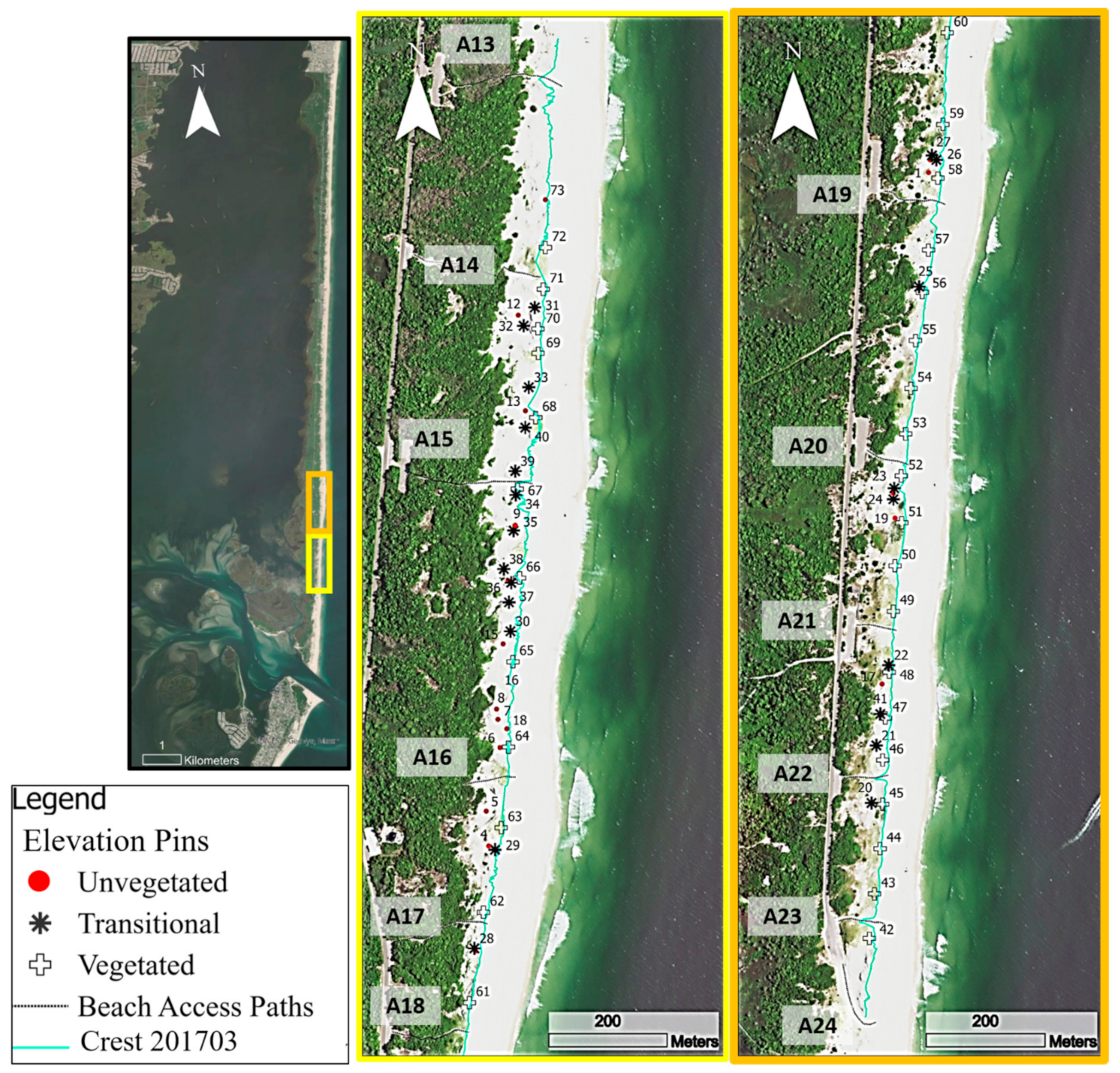
2.1. Study Site
2.2. Microscale Metrics: Elevation Pins
2.3. Mesoscale Remote Sensing Data Collection
2.4. Mesoscale Metrics Derived from Digital Elevation Models
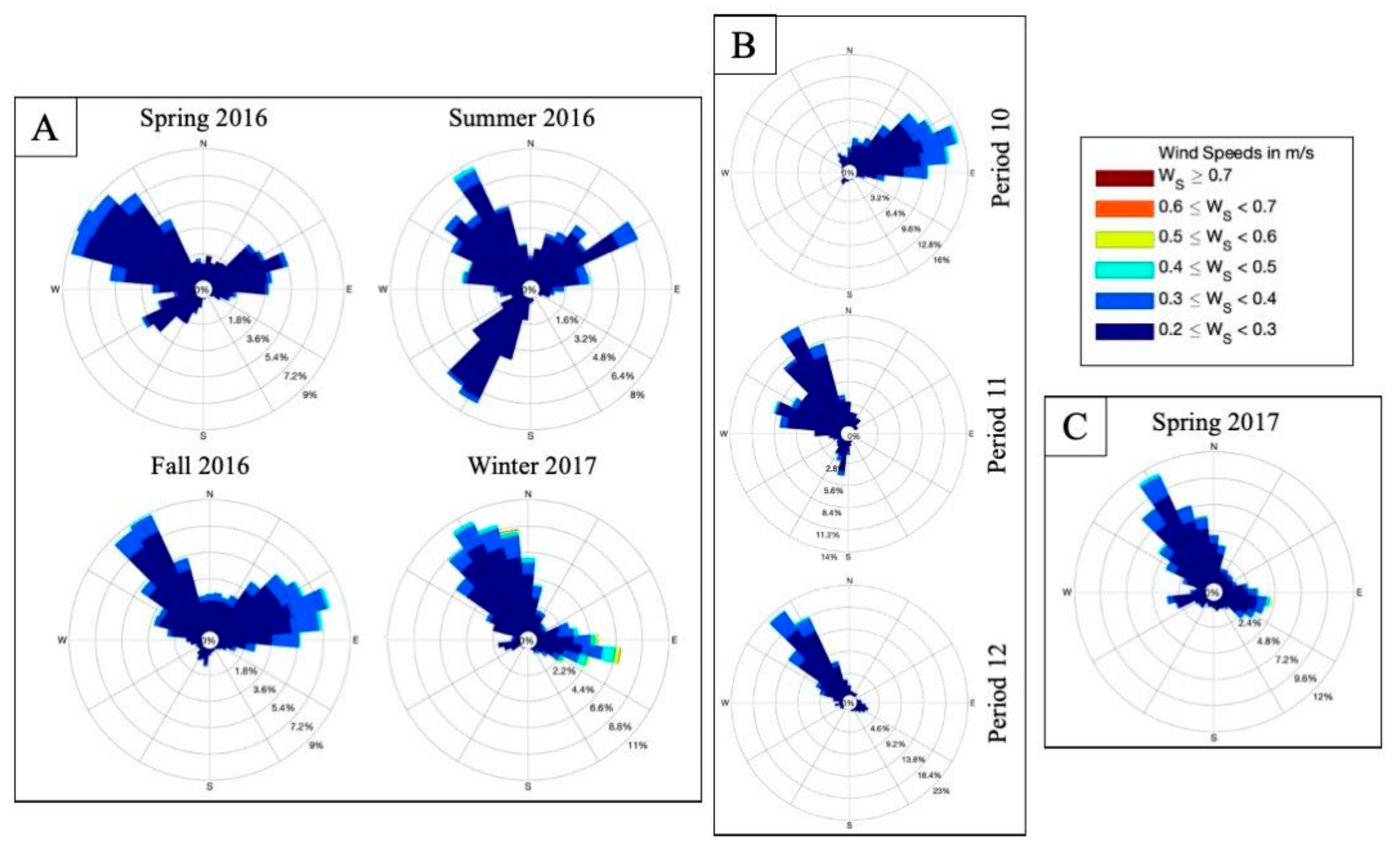
2.5. Sediment Composition and Wind Data
2.6. Statistical Analyses
2.6.1. Microscale Analyses
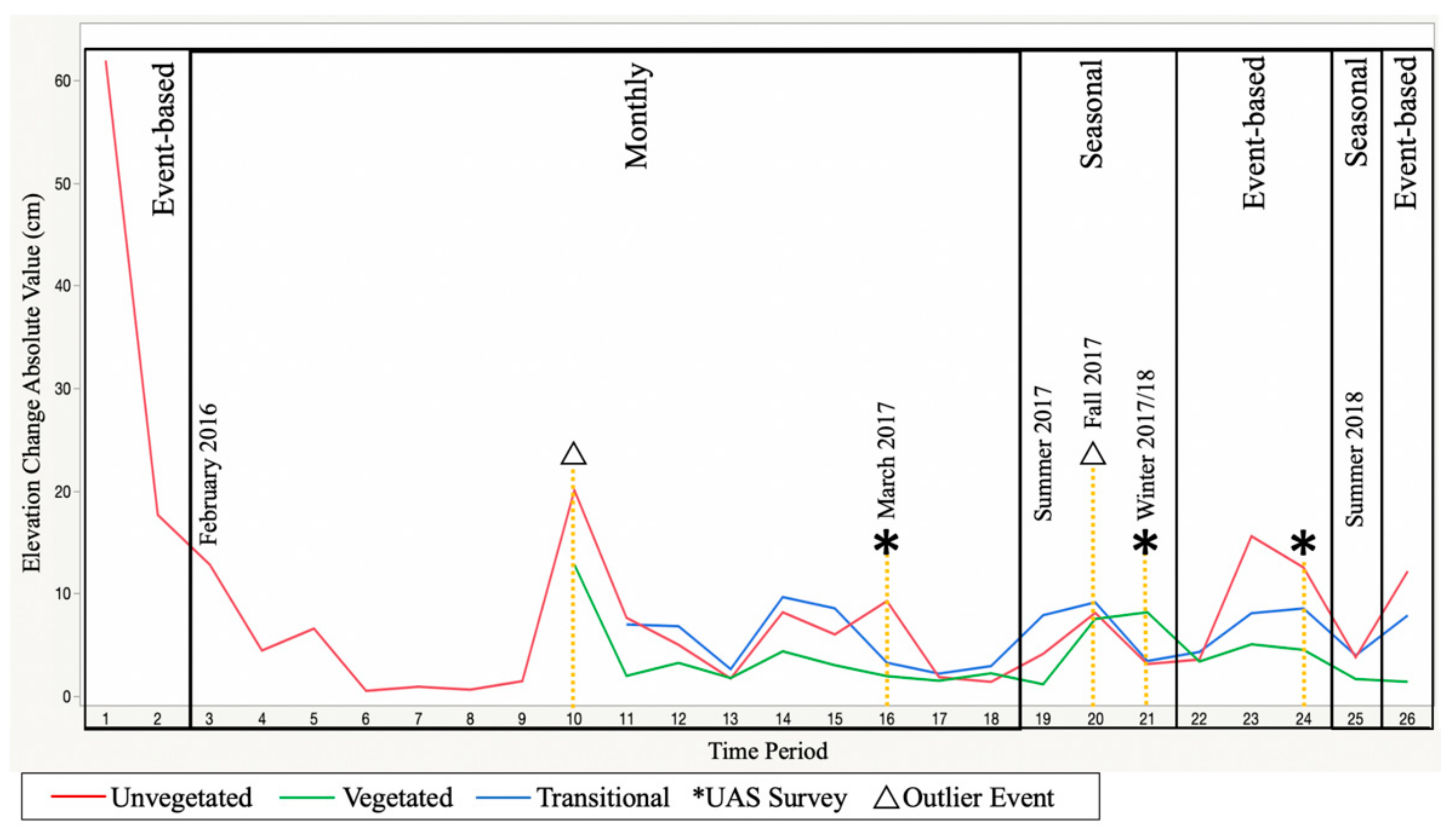
General Variation between Collection Types
Month-to-Month Seasonal Variation Analyses
Vegetation Impact Analyses
2.6.2. Mesoscale Analyses
3. Results
3.1. Site Characteristics during Survey Periods
3.2. Microscale Measured Variation between Collection Types
3.3. Microscale Measured Month-to-Month Seasonal Variation
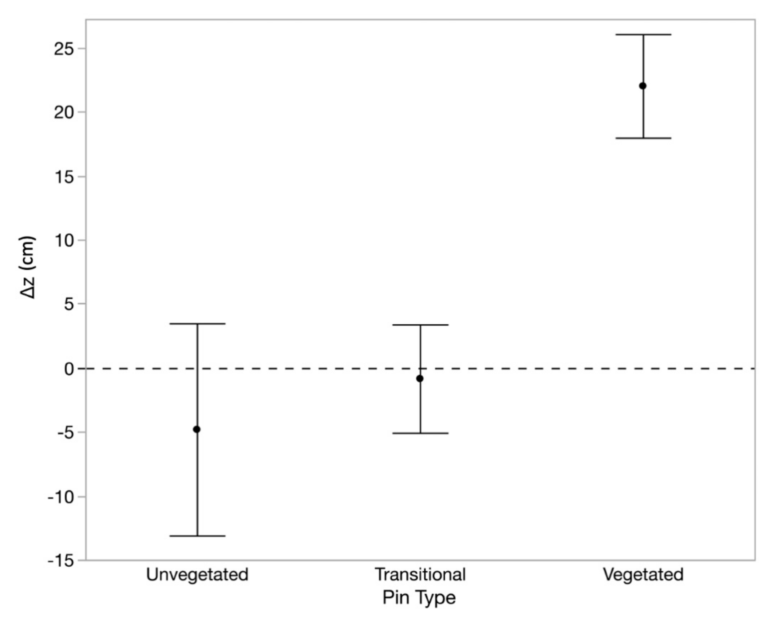
3.4. Impacts of Vegetation on Microscale Measurements
3.5. Microscale to Mesoscale Metric Linking
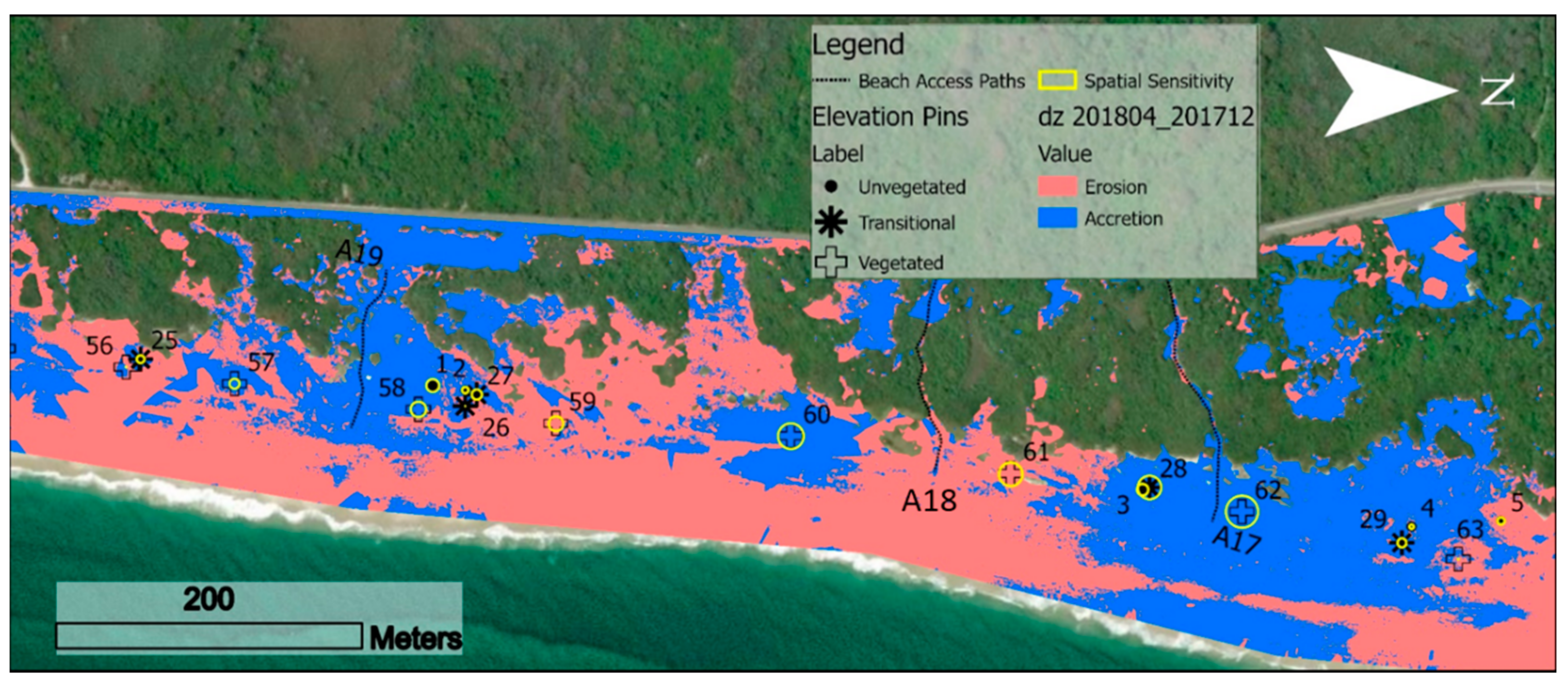
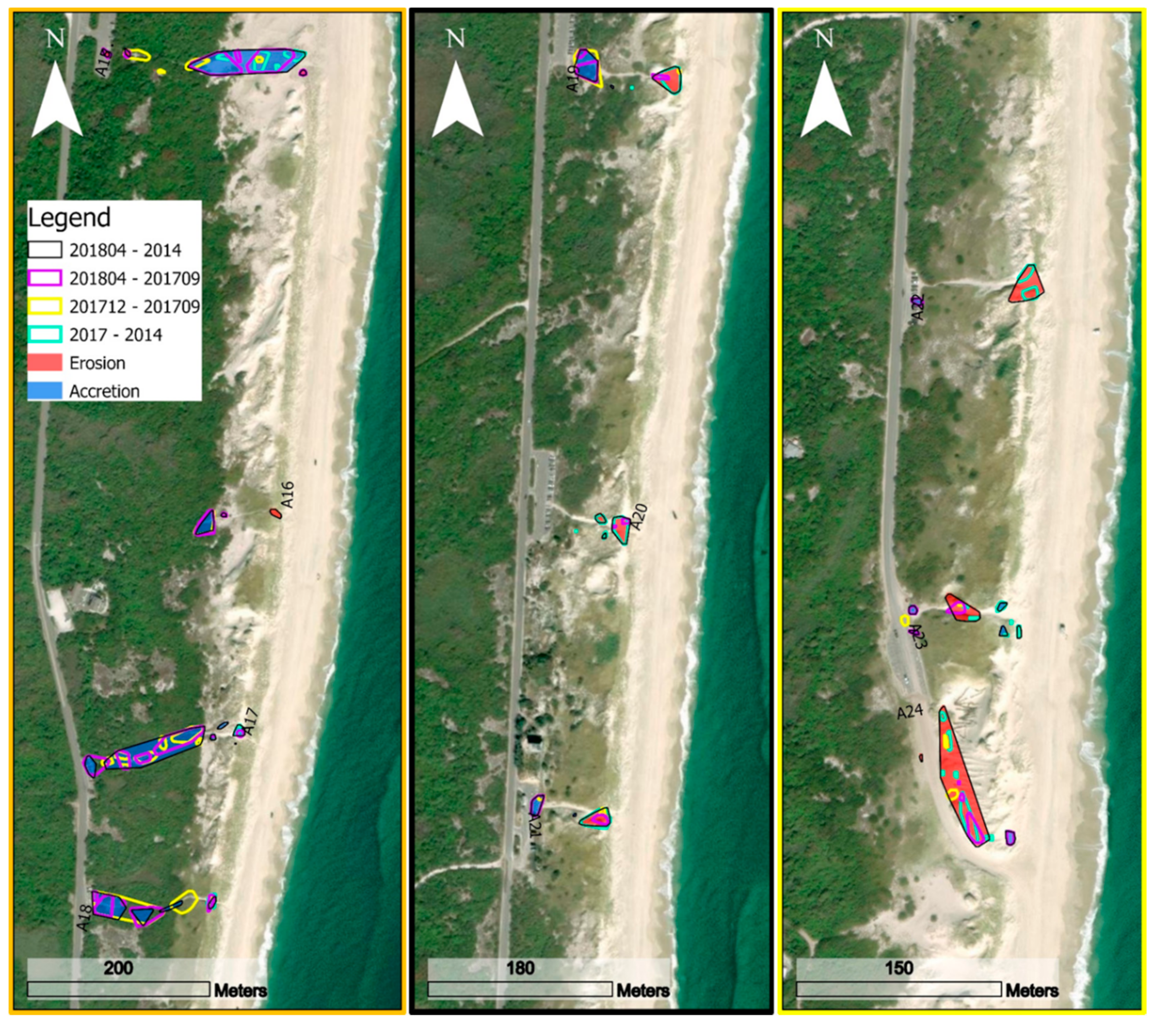
3.6. Beach Access Path Impacts on Local Topographic Change
4. Discussion
5. Conclusions
Supplementary Materials
Author Contributions
Funding
Data Availability Statement
Acknowledgments
Conflicts of Interest
References
- IPCC (Intergovernmental Panel on Climate Change). Climate Change 2014: Synthesis Report. Core Writing Team. 2014, pp. 1–151. Available online: https://www.ipcc.ch/site/assets/uploads/2018/05/SYR_AR5_FINAL_full_wcover.pdf (accessed on 5 November 2021).
- Arneth, A.; Barbosa, H.; Benton, T.; Calvin, K.; Calvo, E.; Connors, S.; Cowie, A.; Davin, E.; Denton, F.; van Diemen, R.; et al. Summary for Policy Makers. Intergovernmental Panel on Climate Change (IPCC). 2019. Available online: https://www.ipcc.ch/site/assets/uploads/sites/4/2019/12/02_Summary-for-Policymakers_SPM.pdf (accessed on 5 November 2021).
- Hesp, P. The Formation of Sand Beach Ridges and Foredunes. Spat. Accuracy 1984, 15, 289–291. [Google Scholar]
- Davenport, J.; Davenport, J.L. The Impact of Tourism and Personal Leisure Transport on Coastal Environments: A Review. Estuar. Coast. Shelf Sci. 2006, 67, 280–292. [Google Scholar] [CrossRef]
- Elko, N.; Brodie, K.; Stockdon, H.; Nordstrom, K. Dune Management Challenges on Developed Coasts. Shore Beach 2016, 84, 15–28. [Google Scholar]
- Hauer, M.E.; Evans, J.M.; Mishra, D.R. Millions Projected to Be at Risk from Sea-Level Rise in the Continental United States. Nat. Clim. Chang. 2016, 6, 691–695. [Google Scholar] [CrossRef]
- Biel, R.G.; Hacker, S.D.; Ruggiero, P.; Cohn, N.; Seabloom, E.W. Coastal Protection and Conservation on Sandy Beaches and Dunes: Context-Dependent Tradeoffs in Ecosystem Service Supply. Ecosphere 2017, 8, e01791. [Google Scholar] [CrossRef]
- Sallenger, J.A.H. Storm Impact Scale for Barrier Islands. J. Coast Res. 2000, 16, 890–895. [Google Scholar] [CrossRef]
- Stallins, J.A.; Parker, A.J. The Influence of Complex Systems Interactions on Barrier Island Dune Vegetation Pattern and Process. Ann. Assoc. Am. Geogr. 2003, 93, 13–29. [Google Scholar] [CrossRef]
- Doran, K.S.; Stockdon, H.F.; Sopkin, K.L.; Thompson, D.M.; Plant, N.G. National Assessment of Hurricane-Induced Coastal Erosion Hazards: Mid-Atlantic Coast. In U.S. Geological Survey Open-File Report; U.S. Geological Survey: Reston, VA, USA, 2013; 28p. [Google Scholar]
- Barone, D.A.; McKenna, K.K.; Farrell, S.C. Hurricane Sandy: Beach-Dune Performance at New Jersey Beach Profile Network Sites. Shore Beach 2014, 82, 13–23. [Google Scholar]
- Houser, C.; Wernette, P.; Rentschlar, E.; Jones, H.; Hammond, B.; Trimble, S. Post-Storm Beach and Dune Recovery: Implications for Barrier Island Resilience. Geomorphology 2015, 234, 54–63. [Google Scholar] [CrossRef]
- Dohner, S.M.; Trembanis, A.C.; Miller, D.C. A Tale of Three Storms: Morphologic Response of Broadkill Beach, Delaware, Following Superstorm Sandy, Hurricane Joaquin, and Winter Storm Jonas. Shore Beach 2016, 84, 3. [Google Scholar]
- Dohner, S.M.; Pilegard, T.C.; Trembanis, A.C. Coupling Traditional and Emergent Technologies for Improved Coastal Zone Mapping. Estuaries Coasts 2020, 1–23. [Google Scholar] [CrossRef]
- Delgado-Fernandez, I.; Davidson-Arnott, R. Meso-Scale Aeolian Sediment Input to Coastal Dunes: The Nature of Aeolian Transport Events. Geomorphology 2011, 126, 217–232. [Google Scholar] [CrossRef] [Green Version]
- Jackson, N.L.; Nordstrom, K.F. Aeolian Sediment Transport on a Recovering Storm-Eroded Foredune with Sand Fences. Earth Surf. Process. Landf. 2018, 43, 1310–1320. [Google Scholar] [CrossRef]
- Nordstrom, K.F.; Jackson, N.L. Offshore Aeolian Sediment Transport across a Human-Modified Foredune. Earth Surf. Proc. Land. 2018, 43, 195–201. [Google Scholar] [CrossRef] [Green Version]
- Gabarrou, S.; Cozannet, G.L.; Parteli, E.J.R.; Pedreros, R.; Guerber, E.; Millescamps, B.; Mallet, C.; Oliveros, C. Modelling the Retreat of a Coastal Dune under Changing Winds. J. Coast. Res. 2018, 85, 166–170. [Google Scholar] [CrossRef]
- Houser, C.; Hapke, C.; Hamilton, S. Controls on Coastal Dune Morphology, Shoreline Erosion and Barrier Island Response to Extreme Storms. Geomorphology 2008, 100, 223–240. [Google Scholar] [CrossRef]
- Houser, C.; Mathew, S. Alongshore Variation in Foredune Height in Response to Transport Potential and Sediment Supply: South Padre Island, Texas. Geomorphology 2011, 125, 62–72. [Google Scholar] [CrossRef]
- Keijsers, J.G.S.; Poortinga, A.; Riksen, M.J.P.M.; Maroulis, J. Spatio-Temporal Variability in Accretion and Erosion of Coastal Foredunes in the Netherlands: Regional Climate and Local Topography. PLoS ONE 2014, 9, e91115. [Google Scholar] [CrossRef] [Green Version]
- Keijsers, J.G.S.; Groot, A.V.D.; Riksen, M.J.P.M. Modeling the Biogeomorphic Evolution of Coastal Dunes in Response to Climate Change. J. Geophys. Res. Earth Surf. 2016, 121, 1161–1181. [Google Scholar] [CrossRef] [Green Version]
- Bryant, D.B.; Bryant, M.A.; Sharp, J.A.; Bell, G.L.; Moore, C. The Response of Vegetated Dunes to Wave Attack. Coast. Eng. 2019, 152, 103506. [Google Scholar] [CrossRef]
- Goldsmith, V.; Rosen, P.; Gertner, Y. Eolian transport measurements, winds, and comparison with theoretical transport on Israeli coastal dunes. In Coastal Dunes: Processes and Morphology; Nordstrom, K., Psuty, N., Carter, R., Eds.; Wiley & Sons, Ltd.: London, UK, 1991; Volume 5, pp. 79–101. [Google Scholar]
- Jackson, N.L.; Nordstrom, K.F. Aeolian Transport of Sediment on a Beach during and after Rainfall, Wildwood, NJ, USA. Geomorphology 1998, 22, 151–157. [Google Scholar] [CrossRef]
- Delgado-Fernandez, I.; Davidson-Arnott, R.; Bauer, B.O.; Walker, I.J.; Ollerhead, J.; Rhew, H. Assessing Aeolian Beach-Surface Dynamics Using a Remote Sensing Approach. Earth Surf. Process. Landf. 2012, 37, 1651–1660. [Google Scholar] [CrossRef] [Green Version]
- Nordstrom, K.F.; Jackson, N.L. The Role of Wind Direction in Eolian Transport on a Narrow Sandy Beach. Earth Surf. Proc. Land. 1993, 18, 675–685. [Google Scholar] [CrossRef]
- Arens, S.M. Rates of Aeolian Transport on a Beach in a Temperate Humid Climate. Geomorphology 1996, 17, 3–18. [Google Scholar] [CrossRef] [Green Version]
- Gares, P.A.; Nordstrom, K.F. A Cyclic Model of Foredune Blowout Evolution for a Leeward Coast: Island Beach, New Jersey. Ann. Assoc. Am. Geogr. 1995, 85, 1–20. [Google Scholar] [CrossRef]
- Bauer, B.O.; Davidson-Arnott, R.G.D.; Walker, I.J.; Hesp, P.A.; Ollerhead, J. Wind Direction and Complex Sediment Transport Response across a Beach-Dune System. Earth Surf. Proc. Land. 2012, 37, 1661–1677. [Google Scholar] [CrossRef]
- Bauer, B.O.; Hesp, P.A.; Walker, I.J.; Davidson-Arnott, R.G.D. Sediment Transport (Dis)Continuity across a Beach–Dune Profile during an Offshore Wind Event. Geomorphology 2015, 245, 135–148. [Google Scholar] [CrossRef] [Green Version]
- Moreno-Casasola, P. Sand Movement as a Factor in the Distribution of Plant Communities in a Coastal Dune System. Vegetatio 1986, 65, 67–76. [Google Scholar] [CrossRef]
- Olson, J.S. Lake Michigan Dune Development 1. Wind-Velocity Profiles. J. Geol. 1958, 66, 254–263. [Google Scholar] [CrossRef]
- Zarnetske, P.L.; Hacker, S.D.; Seabloom, E.W.; Ruggiero, P.; Killian, J.R.; Maddux, T.B.; Cox, D. Biophysical Feedback Mediates Effects of Invasive Grasses on Coastal Dune Shape. Ecology 2012, 93, 1439–1450. [Google Scholar] [CrossRef] [PubMed]
- Keijsers, J.G.S.; Groot, A.V.D.; Riksen, M.J.P.M. Vegetation and Sedimentation on Coastal Foredunes. Geomorphology 2015, 228, 723–734. [Google Scholar] [CrossRef]
- Ashkenazy, Y.; Shilo, E. Sand Dune Albedo Feedback. Geosciences 2018, 8, 82. [Google Scholar] [CrossRef] [Green Version]
- Charbonneau, B.R.; Dohner, S.M.; Wnek, J.P.; Barber, D.; Zarnetske, P.L.; Casper, B.B. Vegetation Effects on Coastal Foredune Initiation: Wind Tunnel Experiments and Field Validation for Three Dune-Building Plants. Geomorphology 2021, 378, 107594. [Google Scholar] [CrossRef]
- Charbonneau, B.R.; Wootton, L.S.; Wnek, J.P.; Langley, J.A.; Posner, M.A. A Species Effect on Storm Erosion: Invasive Sedge Stabilized Dunes More than Native Grass during Hurricane Sandy. J. Appl. Ecol. 2017, 54, 1385–1394. [Google Scholar] [CrossRef] [Green Version]
- da Silva, G.M.; Hesp, P.; Peixoto, J.; Dillenburg, S.R. Foredune Vegetation Patterns and Alongshore Environmental Gradients: Moçambique Beach, Santa Catarina Island, Brazil. Earth Surf. Process. Landf. 2008, 33, 1557–1573. [Google Scholar] [CrossRef]
- Hesp, P.A.; Dong, Y.; Cheng, H.; Booth, J.L. Wind Flow and Sedimentation in Artificial Vegetation: Field and Wind Tunnel Experiments. Geomorphology 2019, 337, 165–182. [Google Scholar] [CrossRef]
- Arens, S.M. Patterns of Sand Transport on Vegetated Foredunes. Geomorphology 1996, 17, 339–350. [Google Scholar] [CrossRef] [Green Version]
- Hesp, P. Foredunes and Blowouts: Initiation, Geomorphology and Dynamics. Geomorphology 2002, 48, 245–268. [Google Scholar] [CrossRef]
- Sun, Y.; Hasi, E.; Liu, M.; Du, H.; Guan, C.; Tao, B. Airflow and Sediment Movement within an Inland Blowout in Hulun Buir Sandy Grassland, Inner Mongolia, China. Aeolian Res. 2016, 22, 13–22. [Google Scholar] [CrossRef]
- Smith, A.; Gares, P.A.; Wasklewicz, T.; Hesp, P.A.; Walker, I.J. Three Years of Morphologic Changes at a Bowl Blowout, Cape Cod, USA. Geomorphology 2017, 295, 452–466. [Google Scholar] [CrossRef] [Green Version]
- Harris, C. Wind Speed and Sand Movement in a Coastal Dune Environment. Area 1974, 6, 243–249. [Google Scholar]
- Gares, P.A. Topographic Changes Associated with Coastal Dune Blowouts at Island Beach State Park, New Jersey. Earth Surf. Process. Landf. 1992, 17, 589–604. [Google Scholar] [CrossRef]
- Cooper, W.S. Coastal Sand Dunes of Oregon and Washington. Geol. Soc. Am. Mem. 1958, 72, 170. [Google Scholar] [CrossRef] [Green Version]
- Frosini, S.; Lardicci, C.; Balestri, E. Global Change and Response of Coastal Dune Plants to the Combined Effects of Increased Sand Accretion (Burial) and Nutrient Availability. PLoS ONE 2012, 7, e47561. [Google Scholar] [CrossRef] [PubMed] [Green Version]
- Charbonneau, B. From The Sand They Rise: Post-Storm Foredune Plant Recolonization and Its Biogeomorphic Implications. Ph.D. Thesis, University of Pennsylvania, Philadelphia, PA, USA, 2019. [Google Scholar]
- Lichter, J. Colonization Constraints during Primary Succession on Coastal Lake Michigan Sand Dunes. J. Ecol. 2000, 88, 825–839. [Google Scholar] [CrossRef]
- Johnson, E.A.; Miyanishi, K. Coastal dune succession and the reality of dune processes. In Plant Disturbance Ecology; Plant Disturbance Ecology; Elsevier: London, UK, 2007; pp. 249–282. [Google Scholar]
- Maun, M.A.; Lapierre, J. Effects of Burial by Sand on Seed Germination and Seedling Emergence of Four Dune Species. Am. J. Bot. 1986, 73, 450–455. [Google Scholar] [CrossRef]
- Moore, L.J. Shoreline Mapping Techniques. J. Coast. Res. 2000, 16, 111–124. [Google Scholar] [CrossRef]
- Hamylton, S.M. Spatial Analysis of Coastal Environments; Cambridge University Press: Cambridge, UK, 2017. [Google Scholar]
- Harley, M.D.; Turner, I.L.; Kinsela, M.A.; Middleton, J.H.; Mumford, P.J.; Splinter, K.D.; Phillips, M.S.; Simmons, J.A.; Hanslow, D.J.; Short, A.D. Extreme Coastal Erosion Enhanced by Anomalous Extratropical Storm Wave Direction. Sci. Rep. 2017, 7, 6033. [Google Scholar] [CrossRef] [PubMed] [Green Version]
- Elko, N.; Dietrich, C.; Cialone, M.; Stockdon, H.; Bilskie, M.W.; Boyd, B.; Charbonneau, B.R.; Cox, D.; Dresback, K.; Elgar, S.; et al. Advancing the Understanding of Storm Processes and Impacts. Shore Beach 2019, 87, 37–51. [Google Scholar]
- Jackson, N.L.; Nordstrom, K.F. Trends in Research on Beaches and Dunes on Sandy Shores, 1969–2019. Geomorphology 2020, 366, 106737. [Google Scholar] [CrossRef]
- Vinent, O.D.; Moore, L.J. Barrier Island Bistability Induced by Biophysical Interactions. Nat. Clim. Chang. 2015, 5, 158–162. [Google Scholar] [CrossRef]
- Spore, N.; Brodie, K.; Swann, C. Automated Feature Extraction of Foredune Morphology from Terrestrial Lidar Data. AGU Fall Meeting Abstracts. 2014, p. EP31B-3558. Available online: https://ui.adsabs.harvard.edu/abs/2014AGUFMEP31B3558S/abstract (accessed on 5 November 2021).
- Ruiz-Martínez, G.; Rivillas-Ospina, G.; Mariño-Tapia, I.; Posada-Vanegas, G. SANDY: A Matlab Tool to Estimate the Sediment Size Distribution from a Sieve Analysis. Comput. Geosci. 2016, 92, 104–116. [Google Scholar] [CrossRef]
- Pereira, D. Wind Rose. MATLAB Central File Exchang. 2021. Available online: https://www.mathworks.com/matlabcentral/fileexchange/47248-wind-rose (accessed on 10 September 2021).
- MATLAB. MATLAB and Statistics and Machine Learning Toolbox Release 2018a; MATLAB: Natick, MA, USA, 2018. [Google Scholar]
- Zingg, A. Wind Tunnel Studies of The Movement of Sedimentary Material. In Proceedings of the 5th Hydraulics Conference, Iowa City, IA, USA, 9–11 June 1953; Iowa institute of Hydraulic Research: Iowa City, IA, USA; Volume 34, pp. 11–135. [Google Scholar]
- Bagnold, R.A. The Physics of Blown Sand and Desert Dunes; William Morrow and Company: New York, NY, USA, 1943. [Google Scholar]
- Hesp, P.; Hyde, R. Flow Dynamics and Geomorphology of a Trough Blowout. Sedimentology 1996, 43, 505–525. [Google Scholar] [CrossRef]
- Hesp, P.A. Flow Dynamics in a Trough Blowout. Bound.-Layer Meteorol. 1996, 77, 305–330. [Google Scholar] [CrossRef]
- Hesp, P. Morphodynamics of Incipient Foredunes in New South Wales, Australia. In Eolian Sediments and Processes; Elsevier: Amsterdam, The Netherlands, 1983; Volume 38, pp. 325–342. ISBN 9780444422330. [Google Scholar]
- Hesp, P.A. Foredune formation in SE Australia. In Coastal Geomorphology in Australia; Thom, B.G., Ed.; Academic Press: Cambridge, MA, USA, 1984; pp. 60–97. [Google Scholar]
- Jagschitz, J.A.; Wakefield, R.C. How to Build and Save Beaches and Dunes; College of Resource Development, University of Rhode Island: Kingston, RI, USA, 1971. [Google Scholar]
- Hacker, S.D.; Jay, K.R.; Cohn, N.; Goldstein, E.B.; Hovenga, P.A.; Itzkin, M.; Moore, L.J.; Mostow, R.S.; Mullins, E.V.; Ruggiero, P. Species-Specific Functional Morphology of Four US Atlantic Coast Dune Grasses: Biogeographic Implications for Dune Shape and Coastal Protection. Diversity 2019, 11, 82. [Google Scholar] [CrossRef] [Green Version]
- Zarnetske, P.L.; Ruggiero, P.; Seabloom, E.W.; Hacker, S.D. Coastal Foredune Evolution: The Relative Influence of Vegetation and Sand Supply in the US Pacific Northwest. J. R. Soc. Interface 2015, 12, 20150017. [Google Scholar] [CrossRef] [Green Version]
- Biel, R.G.; Hacker, S.D.; Ruggiero, P. Elucidating Coastal Foredune Ecomorphodynamics in the U.S. Pacific Northwest via Bayesian Networks. J. Geophys. Res. Earth Surf. 2019, 124, 1919–1938. [Google Scholar] [CrossRef]
- Walker, I.J.; Davidson-Arnott, R.G.D.; Bauer, B.O.; Hesp, P.A.; Delgado-Fernandez, I.; Ollerhead, J.; Smyth, T.A.G. Scale-Dependent Perspectives on the Geomorphology and Evolution of Beach-Dune Systems. Earth-Sci. Rev. 2017, 171, 220–253. [Google Scholar] [CrossRef]
- Česnulevičius, A.; Bautrėnas, A.; Bevainis, L.; Ovodas, D.; Papšys, K. Applicability of Unmanned Aerial Vehicles in Research on Aeolian Processes. Pure Appl. Geophys. 2018, 175, 3179–3191. [Google Scholar] [CrossRef]
- Solazzo, D.; Sankey, J.; Sankey, T. Mapping and Measuring Aeolian Sand Dunes with Photogrammetry and LiDAR from Unmanned Aerial Vehicles (UAV) and Multispectral Satellite Imagery on the Paria Plateau, AZ, USA. Geomorphology 2018, 319, 174–185. [Google Scholar] [CrossRef]
- Baird, D.J.; Brown, S.S.; Lagadic, L.; Liess, M.; Maltby, L.; Moreira-Santos, M.; Schulz, R.; Scott, G.I. In Situ-Based Effects Measures: Determining the Ecological Relevance of Measured Responses. Integr. Environ. Assess. Manag. 2007, 3, 259–267. [Google Scholar] [CrossRef] [PubMed]
- Feagin, R.A.; Figlus, J.; Zinnert, J.C.; Sigren, J.; Martínez, M.L.; Silva, R.; Smith, W.K.; Cox, D.; Young, D.R.; Carter, G. Going with the Flow or against the Grain? The Promise of Vegetation for Protecting Beaches, Dunes, and Barrier Islands from Erosion. Front. Ecol. Environ. 2015, 13, 203–210. [Google Scholar] [CrossRef] [Green Version]
- Laporte-Fauret, Q.; Castelle, B.; Michalet, R.; Marieu, V.; Bujan, S.; Rosebery, D. Morphological and Ecological Responses of a Managed Coastal Sand Dune to Experimental Notches. Sci. Total Environ. 2021, 782, 146813. [Google Scholar] [CrossRef]
- Castelle, B.; Laporte-Fauret, Q.; Marieu, V.; Michalet, R.; Rosebery, D.; Bujan, S.; Lubac, B.; Bernard, J.-B.; Valance, A.; Dupont, P.; et al. Nature-Based Solution along High-Energy Eroding Sandy Coasts: Preliminary Tests on the Reinstatement of Natural Dynamics in Reprofiled Coastal Dunes. Water 2018, 11, 2518. [Google Scholar] [CrossRef] [Green Version]
- Hesp, P.A.; Martínez, M.L. Plant Disturbance Ecology. Disturbance Processes and Dynamics in Coastal Dunes; Elsevier: Amsterdam, The Netherlands, 2007; ISBN 9780120887781. [Google Scholar]
- Gallego-Fernández, J.B.; Martínez, M.L. Environmental Filtering and Plant Functional Types on Mexican Foredunes along the Gulf of Mexico. Écoscience 2015, 18, 52–62. [Google Scholar] [CrossRef]
- Purvis, K.G.; Gramling, J.M.; Murren, C.J. Assessment of Beach Access Paths on Dune Vegetation: Diversity, Abundance, and Cover. J. Coast. Res. 2015, 315, 1222–1228. [Google Scholar] [CrossRef]
- Prisco, I.; Acosta, A.T.R.; Stanisci, A. A Bridge between Tourism and Nature Conservation: Boardwalks Effects on Coastal Dune Vegetation. J. Coast. Conserv. 2021, 25, 14. [Google Scholar] [CrossRef]
- Riksen, M.J.P.M.; Goossens, D.; Huiskes, H.P.J.; Krol, J.; Slim, P.A. Constructing Notches in Foredunes: Effect on Sediment Dynamics in the Dune Hinterland. Geomorphology 2016, 253, 340–352. [Google Scholar] [CrossRef]
- Ruessink, B.G.; Arens, S.M.; Kuipers, M.; Donker, J.J.A. Coastal Dune Dynamics in Response to Excavated Foredune Notches. Aeolian Res. 2018, 31, 3–17. [Google Scholar] [CrossRef]
- Pye, K.; Blott, S. Dune Rejuvenation Trials Overview Report. Natural Resources Wales Evidence Report Series Report No: 296; Kenneth Py Associates Ltd.: Reading, UK, 2016. [Google Scholar]
- Stallins, J.A. Scale, Causality, and the New Organism-Environment Interaction. Geoforum 2012, 43, 427–441. [Google Scholar] [CrossRef]
- Zinnert, J.C.; Stallins, J.A.; Brantley, S.T.; Young, D.R. Crossing Scales: The Complexity of Barrier-Island Processes for Predicting Future Change. BioScience 2017, 67, 39–52. [Google Scholar] [CrossRef]
- Stallins, J.A.; Corenblit, D. Interdependence of Geomorphic and Ecologic Resilience Properties in a Geographic Context. Geomorphology 2018, 305, 76–93. [Google Scholar] [CrossRef]
- Monge, J.A.; Stallins, J.A. Properties of Dune Topographic State Space for Six Barrier Islands of the U.S. Southeastern Atlantic Coast. Phys. Geogr. 2016, 37, 452–475. [Google Scholar] [CrossRef]
- Hanley, M.E.; Bouma, T.J.; Mossman, H.L. The Gathering Storm: Optimizing Management of Coastal Ecosystems in the Face of a Climate-Driven Threat. Ann. Bot. 2020, 125, 197–212. [Google Scholar] [CrossRef] [PubMed] [Green Version]
- Stallins, J.A. Geomorphology and Ecology: Unifying Themes for Complex Systems in Biogeomorphology. Geomorphology 2006, 77, 207–216. [Google Scholar] [CrossRef]
- Kim, D.; Yu, K.B.; Park, S.J. Identification and Visualization of Complex Spatial Pattern of Coastal Dune Soil Properties Using GIS-Based Terrain Analysis and Geostatistics. J. Coast. Res. 2008, 4, 50–60. [Google Scholar] [CrossRef]
- Snyder, R.A.; Boss, C.L. Recovery and Stability in Barrier Island Plant Communities. J. Coast. Res. 2002, 18, 530–536. [Google Scholar] [CrossRef]
- Cheplick, G.P. Changes in Plant Abundance on a Coastal Beach Following Two Major Storm Surges 1. J. Torrey Bot. Soc. 2016, 143, 180–191. [Google Scholar] [CrossRef]
- Wolner, C.W.V.; Moore, L.J.; Young, D.R.; Brantley, S.T.; Bissett, S.N.; McBride, R.A. Ecomorphodynamic Feedbacks and Barrier Island Response to Disturbance: Insights from the Virginia Barrier Islands, Mid-Atlantic Bight, USA. Geomorphology 2013, 199, 115–128. [Google Scholar] [CrossRef]
- Wootton, L.S.; Halsey, S.D.; Bevaart, K.; McGough, A.; Ondreicka, J.; Patel, P. When Invasive Species Have Benefits as Well as Costs: Managing Carex Kobomugi (Asiatic Sand Sedge) in New Jersey’s Coastal Dunes. Biol. Invasions 2005, 7, 1017–1027. [Google Scholar] [CrossRef]
- Goldstein, E.B.; Moore, L.J.; Vinent, O.D. Lateral Vegetation Growth Rates Exert Control on Coastal Foredune “Hummockiness” and Coalescing Time. Earth Surf. Dyn. 2017, 5, 417–427. [Google Scholar] [CrossRef] [Green Version]
- Murray, A.B.; Knaapen, M.A.F.; Tal, M.; Kirwan, M.L. Biomorphodynamics: Physical-biological Feedbacks That Shape Landscapes. Water Resour. Res. 2008, 44, W11301. [Google Scholar] [CrossRef]
- Rogers, S.; Manning, I.; Livingstone, W. Comparing the Spatial Accuracy of Digital Surface Models from Four Unoccupied Aerial Systems: Photogrammetry Versus LiDAR. Remote Sens. 2020, 12, 2806. [Google Scholar] [CrossRef]
- Linchant, J.; Lisein, J.; Semeki, J.; Lejeune, P.; Vermeulen, C. Are Unmanned Aircraft Systems (UASs) the Future of Wildlife Monitoring? A Review of Accomplishments and Challenges. Mammal Rev. 2015, 45, 239–252. [Google Scholar] [CrossRef]
- Fitzpatrick, B.P. Unmanned Aerial Systems for Surveying and Mapping: Cost Comparison of UAS Versus Traditional Methods of Data Acquisition. Ph.D. Thesis, University of Southern California, Los Angeles, CA, USA, 2016. [Google Scholar]


| Date | 10-Jun-15 | 09-Oct-15 | 02-Feb-16 | 02-Mar-16 | 31-Mar-16 | 09-May-16 | 08-Jun-16 | 15-Jul-16 | 18-Aug-16 | 12-Sep-16 | 17-Oct-16 | 12-Nov-16 | 09-Dec-16 | 12-Jan-17 | 26-Jan-17 | 28-Feb-17 | 21-Mar-17 | 21-Apr-17 | 24-May-17 | 18-Aug-17 | 13-Nov-17 | 28-Feb-18 | 19-Mar-18 | 05-Apr-18 | 23-May-18 | 16-Aug-18 | 20-Sep-18 |
|---|---|---|---|---|---|---|---|---|---|---|---|---|---|---|---|---|---|---|---|---|---|---|---|---|---|---|---|
| Collection | 1 | 2 | 3 | 4 | 5 | 6 | 7 | 8 | 9 | 10 | 11 | 12 | 13 | 14 | 15 | 16 | 17 | 18 | 19 | 20 | 21 | 22 | 23 | 24 | 25 | 26 | 27 |
| Unvegetated | 12 | 8 | 10 | 10 | 11 | 10 | 12 | 12 | 12 | 12 | 16 | 18 | 17 | 17 | 17 | 18 | 17 | 16 | 16 | 16 | 17 | 17 | 17 | 17 | 18 | 18 | 16 |
| Vegetated | - | - | - | - | - | - | - | - | - | 31 | 31 | 31 | 30 | 31 | 29 | 29 | 30 | 31 | 31 | 28 | 27 | 28 | 29 | 31 | 31 | 31 | 30 |
| Transitional | - | - | - | - | - | - | - | - | - | - | 20 | 21 | 21 | 22 | 22 | 22 | 22 | 21 | 19 | 22 | 21 | 22 | 22 | 19 | 19 | 20 | 19 |
| Period | 1 | 1&2 | 2&3 | 3&4 | 4&5 | 5&6 | 6&7 | 7&8 | 8&9 | 9&10 | 10&11 | 11&12 | 12&13 | 13&14 | 14&15 | 15&16 | 16&17 | 17&18 | 18&19 | 19&20 | 20&21 | 21&22 | 22&23 | 23&24 | 24&25 | 25&26 | 26 |
| Data | Source/Instrument | Dates (yyyy-mm-dd) | Resolution (Grid or Cell Size) | Uncertainty | Analysis |
|---|---|---|---|---|---|
| satellite imagery | USDA NAIP | 7 June 2015 | 1 m | ±6.1 m | map background; mask creation |
| topobathy lidar DEM | USGS, NOAA, CMP, USACE | 2014, September 2017 | 1 m | ±0.09–0.15 m | mesoscale metrics |
| UAS DEM | DJI® Phantom 3 Advanced™, eBee™ SenseFly® | 21 March 2017, 11 December 2017, 22 April 2018 | 0.05 m | ±0.15 m | mesoscale metrics |
| mapped features | Trimble® GeoXT™ GeoExplorer® | 2013–2018 | 0.15 m | ±0.8 m | microscale metrics |
| sediment samples | coring, brab | 2018 | --- | --- | aeolian critical threshold |
| Variation in |Δz| | Statistical Test | Pairwise Comparisons | |
|---|---|---|---|
| Seasonal Test 1: All 6 seasons | transitional = unvegetated and vegetated pins; vegetated < unvegetated | F2,395 = 8.35, p < 0.001 | fall > spring and summer (F3,395 = 7.82, p < 0.0001) |
| Seasonal Test 2: 2017 data | F2,63 = 4.91, p < 0.01 | No pairwise seasonal differences | |
| Seasonal Test 3: 2017 and 2018 Combined | F2,262 = 3.89, p = 0.02 | spring > summer and Fall (F3,262 = 12.70, p < 0.0001) |
| Pin Type | Collection Type | Min Δz | Max Δz | Mean Δz | Mean |Δz| | Accretion Mean Δz | Erosion Mean Δz |
|---|---|---|---|---|---|---|---|
| u | event | −47.4 | 106.7 | 11.2 ± 2.6 | 17.2 ± 2.3 | 23.0 ± 3.5 | −10.3 ± 1.8 |
| transitional | −37.2 | 68.6 | 4.2 ± 1.3 | 7.5 ± 1.1 | 10.4 ± 1.7 | −5.9 ± 1.5 | |
| vegetated | −16.5 | 40.6 | 4.3 ± 0.7 | 5.4 ± 0.6 | 7.0 ± 0.8 | −4.6 ± 1.2 | |
| unvegetated | seasonal | −30.1 | 7.7 | −1.8 ± 0.9 | 3.6 ± 0.7 | 2.7 ± 0.6 | −5.5 ± 1.3 |
| transitional | −40.6 | 29.6 | 1.6 ± 1.0 | 5.0 ± 1.1 | 3.9 ± 1.1 | −6.9 ± 2.0 | |
| vegetated | −54.6 | 33.7 | 2.0 ± 0.8 | 4.4 ± 0.8 | 5.8 ± 1.0 | −6.1 ± 2.4 | |
| unvegetated | monthly | −37.3 | 71.1 | −0.5 ± 0.6 | 4.6 ± 0.5 | 7.1 ± 1.4 | −5.0 ± 0.6 |
| transitional | −36.8 | 35.6 | −1.0 ± 0.7 | 5.3 ± 0.5 | 5.4 ± 0.9 | −6.2 ± 0.7 | |
| vegetated | −17.8 | 27.9 | 0.6 ± 0.3 | 2.4 ± 0.2 | 3.1 ± 0.3 | −3.1 ± 0.4 | |
| unvegetated | total Δz | −40.0 | 41.9 | −4.8 ± 8.3 | 28.2 ± 3.1 | 27.3 ± 4.1 | −28.9 ± 4.6 |
| transitional | −25.4 | 35.6 | −0.8 ± 16.9 | 13.4 ± 2.4 | 11.1 ± 3.7 | −16.2 ± 2.8 | |
| vegetated | −45.7 | 61.6 | 22.0 ± 4.1 | 25.8 ± 3.2 | 26.6 ± 3.3 | −19.1 ± 13.5 |
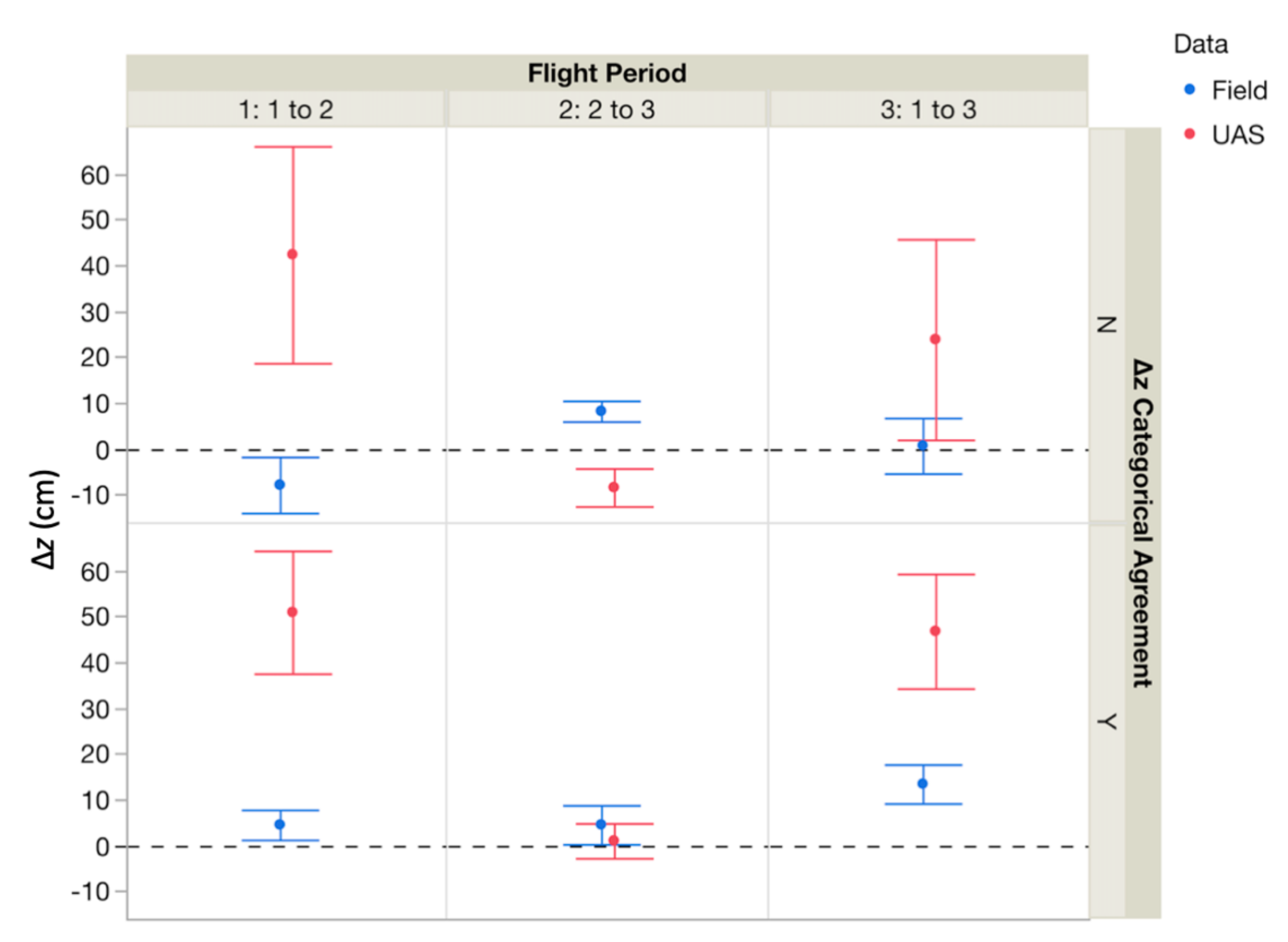
| UAS Surface Δz vs. Actual (Pin) Δz | Mean UAS Δz | Mean Pin Δz | Wilcoxon Test Result | ||
|---|---|---|---|---|---|
| Flights 1 to 2 | instances of categorical incongruence between data types | UAS surface overestimated Δz | 28.96 ± 23.3 cm | -7.83 ± 6.11 cm | Z = 2.31, p = 0.02 |
| Flights 1 to 3 | 23.85 ± 21.88 cm | 0.70 ± 6.05 cm | Z = 0.84, p = 0.40 | ||
| Flights 2 to 3 | UAS surface underestimated Δz | −8.39 ± 4.14 cm | 8.23 ± 2.25 cm | Z = −4.28, p < 0.0001 | |
| Flights 1 to 2 | instances of categorical congruence between data types | UAS surface overestimated Δz | 56.88 ± 13.13 cm | 4.51 ± 3.27 cm | Z = 4.26, p < 0.0001 |
| Flights 1 to 3 | 46.78 ± 12.48 cm | 13.41 ± 4.23 cm | Z = 4.15, p < 0.0001 | ||
| Flights 2 to 3 | UAS surface & actual equal | 2.77 ± 2.83 cm | Z = 4.15, p < 0.0001 | ||
| Survey Period | ||||
|---|---|---|---|---|
| 1: 2014 to September 2017 | 2: September 2016 to December 2017 | 3: December 2017 to April 2018 | 4: 2014 to April 2018 | |
| impact polygons identified (n) | 34 | 24 | 35 | 38 |
| width (m) | 5.4 ± 0.9 | 8.1 ± 1.3 | 8.9 ± 1.2 | 9.9 ± 1.3 |
| length (m) | 11.8 ± 1.8 | 18.3 ± 3.4 | 17.4 ± 2.5 | 27.6 ± 2.4 |
| surface area (m2) | 2677 | 4515 | 6084 | 11,610 |
| orientation (°) | 77.2 ± 8.8 | 84.6 ± 9.2 | 86.4 ± 7.8 | 90.7 ± 7.9 |
Publisher’s Note: MDPI stays neutral with regard to jurisdictional claims in published maps and institutional affiliations. |
© 2021 by the authors. Licensee MDPI, Basel, Switzerland. This article is an open access article distributed under the terms and conditions of the Creative Commons Attribution (CC BY) license (https://creativecommons.org/licenses/by/4.0/).
Share and Cite
Charbonneau, B.R.; Dohner, S.M. Microscale and Mesoscale Aeolian Processes of Sandy Coastal Foredunes from Background to Extreme Conditions. Remote Sens. 2021, 13, 4488. https://doi.org/10.3390/rs13214488
Charbonneau BR, Dohner SM. Microscale and Mesoscale Aeolian Processes of Sandy Coastal Foredunes from Background to Extreme Conditions. Remote Sensing. 2021; 13(21):4488. https://doi.org/10.3390/rs13214488
Chicago/Turabian StyleCharbonneau, Bianca R., and Stephanie M. Dohner. 2021. "Microscale and Mesoscale Aeolian Processes of Sandy Coastal Foredunes from Background to Extreme Conditions" Remote Sensing 13, no. 21: 4488. https://doi.org/10.3390/rs13214488