
Numerical Assessment of Downward Incoming Solar Irradiance in Smoke Influenced Regions—A Case Study in Brazilian Amazon and Cerrado

 ,
,  ,
,  , ,
, ,  ,
, 

Abstract
:
1. Introduction
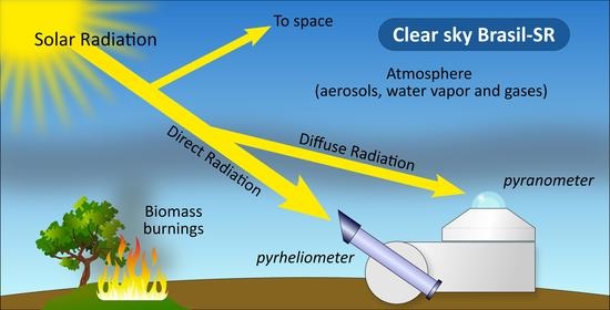
2. BRASIL-SR Model
3. Experimental Data and Methods
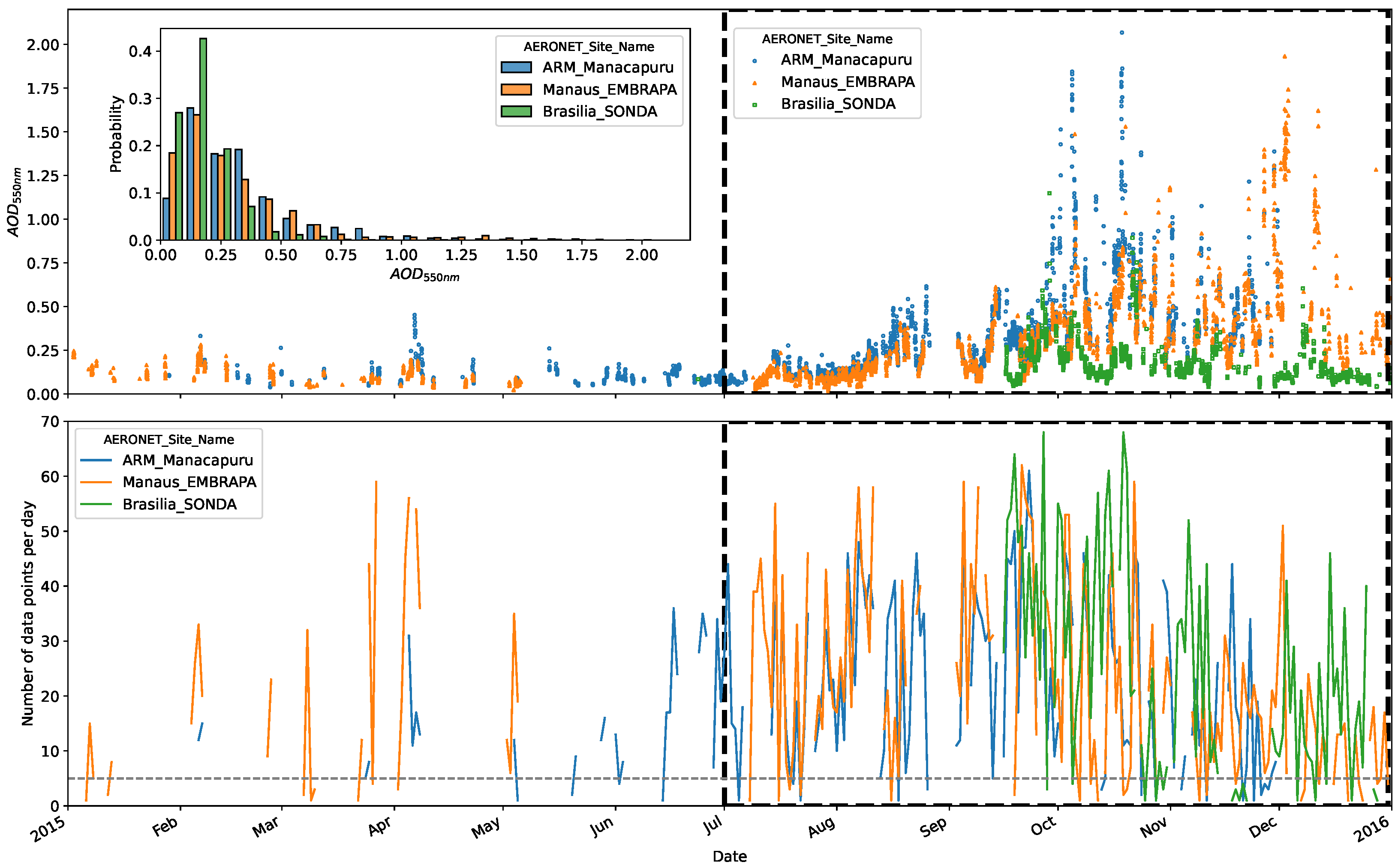
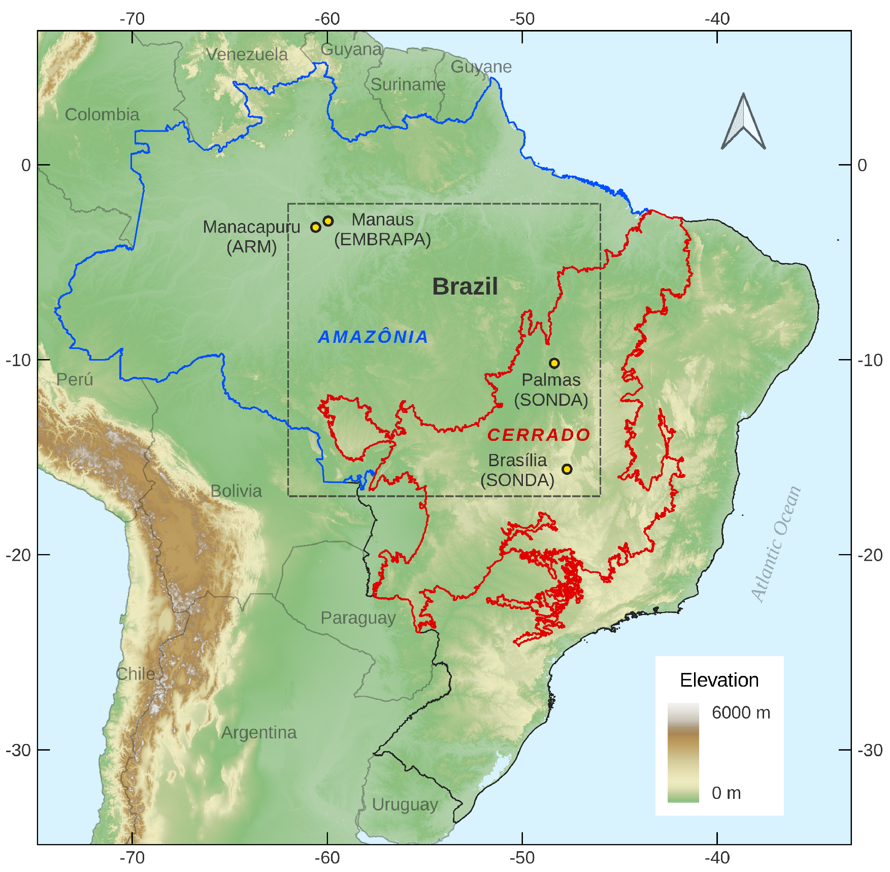
3.1. Observational Data
3.2. BRASIL-SR Input Data and Configuration
3.3. Model Validation
- Mean Bias Difference (MBD)where and are the model outputs and observed values, respectively, is the mean observed value and is the number of clear sky observations.
- Root Mean Square Difference (RMSD)
- Mean Absolute Difference (MAD)
- Kolmogorov-Smirnov integral (KSI)—defined as the integrated differences between the cumulative distribution functions (CDFs) of the model (p) and observational (o) data sets.where is the absolute difference between the two normalized distributions within irradiance interval, and are the minimum and maximum solar irradiance values, and Ac is a characteristic quantity of the distributionfor .
- OVER—statistical parameter similar to KSI, but the integration is calculated only for those CDFs’ differences that exceed the critical limit () of the Kolmogorov-Smirnov method. From Equation (7), it can be notice that OVER is 0 (zero) if the CDFs’ differences always remains below the critical value [62].
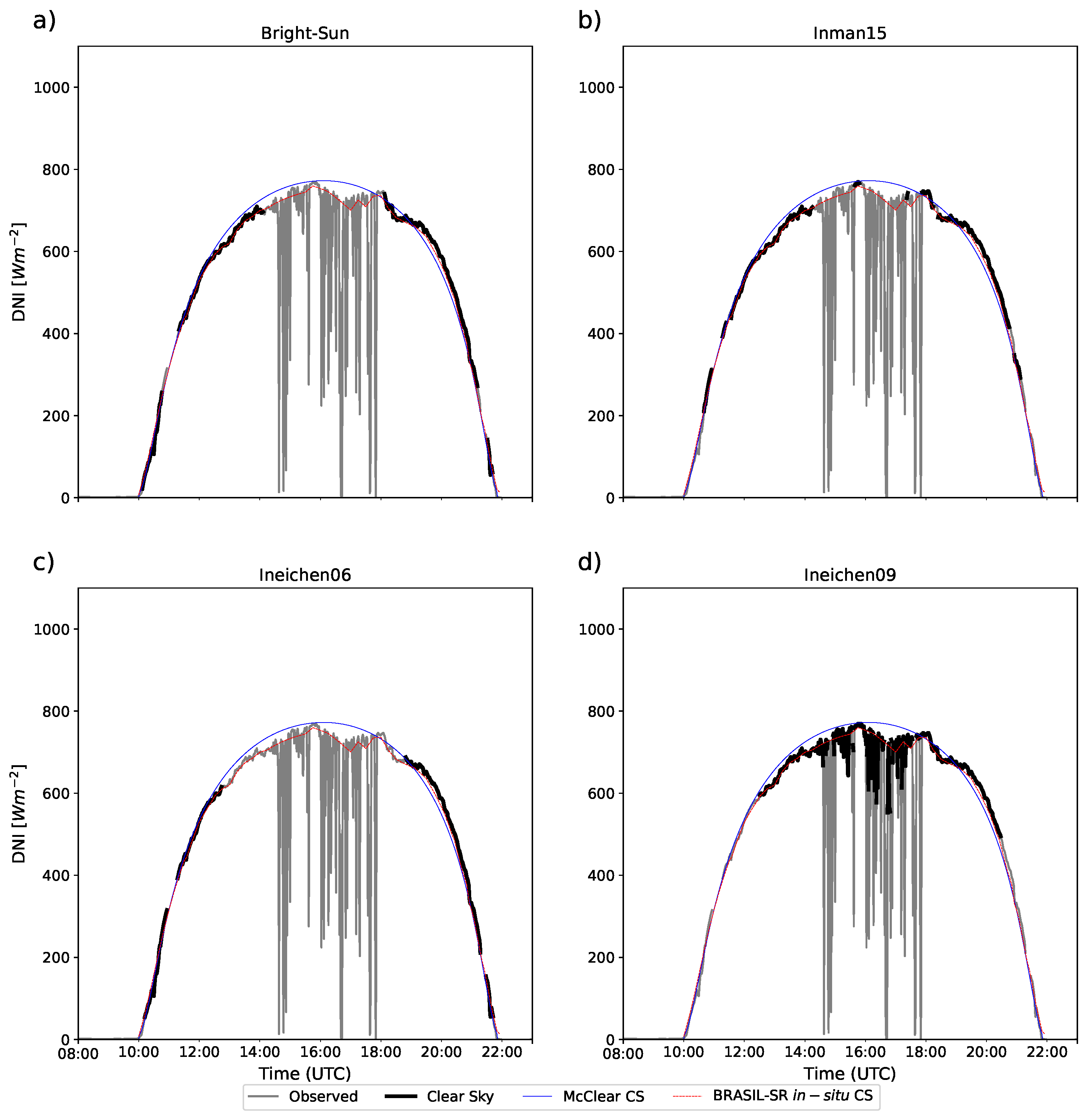
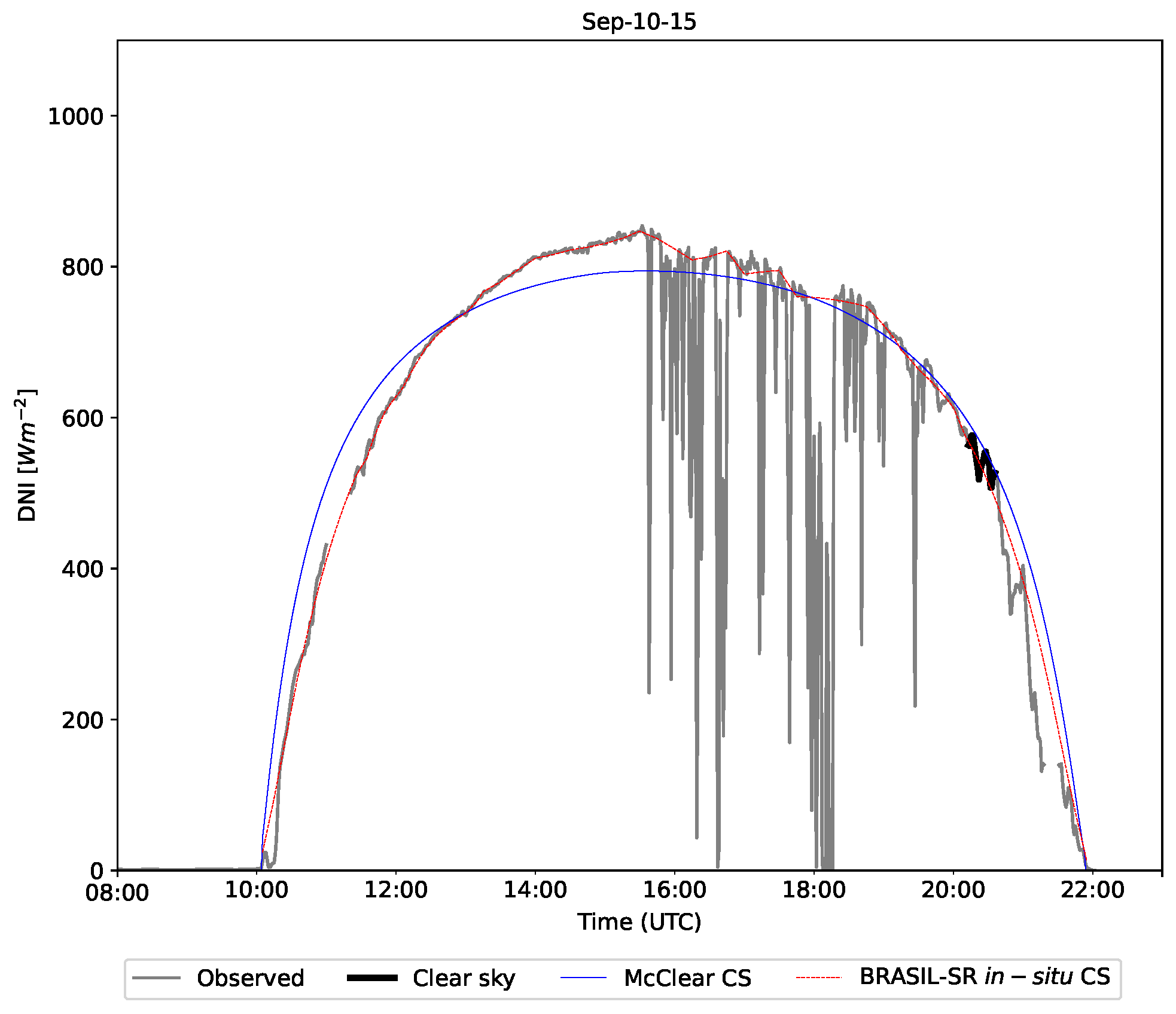
3.4. Selection of Clear-Sky Periods
- (a)
- a DNI threshold—, where the right side represents the DNI in cloudless condition , is the the extraterrestrial solar irradiance, and m is the air mass; and
- (b)
- a DNI variability threshold—the DNI variability remains of variability.
4. Results
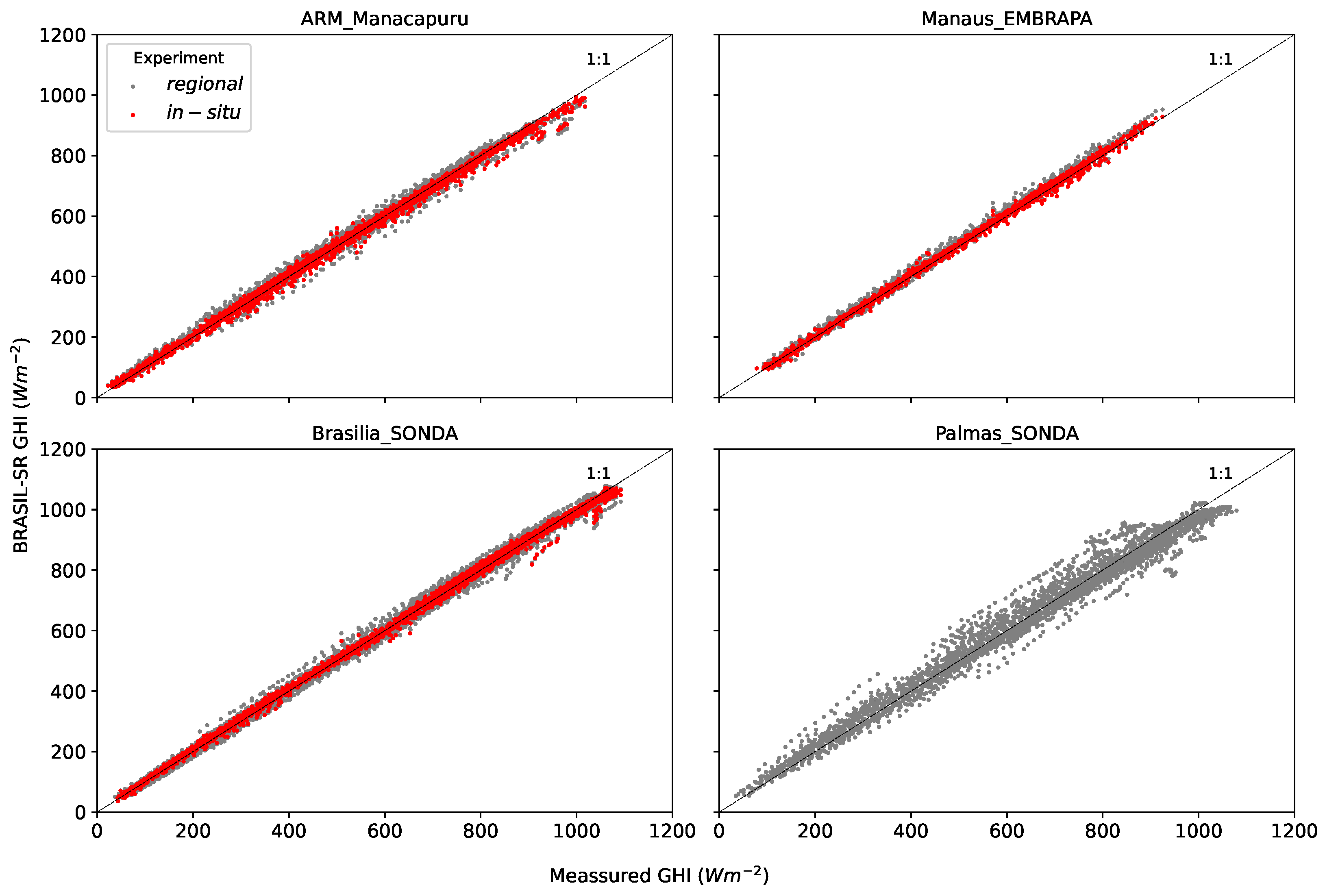
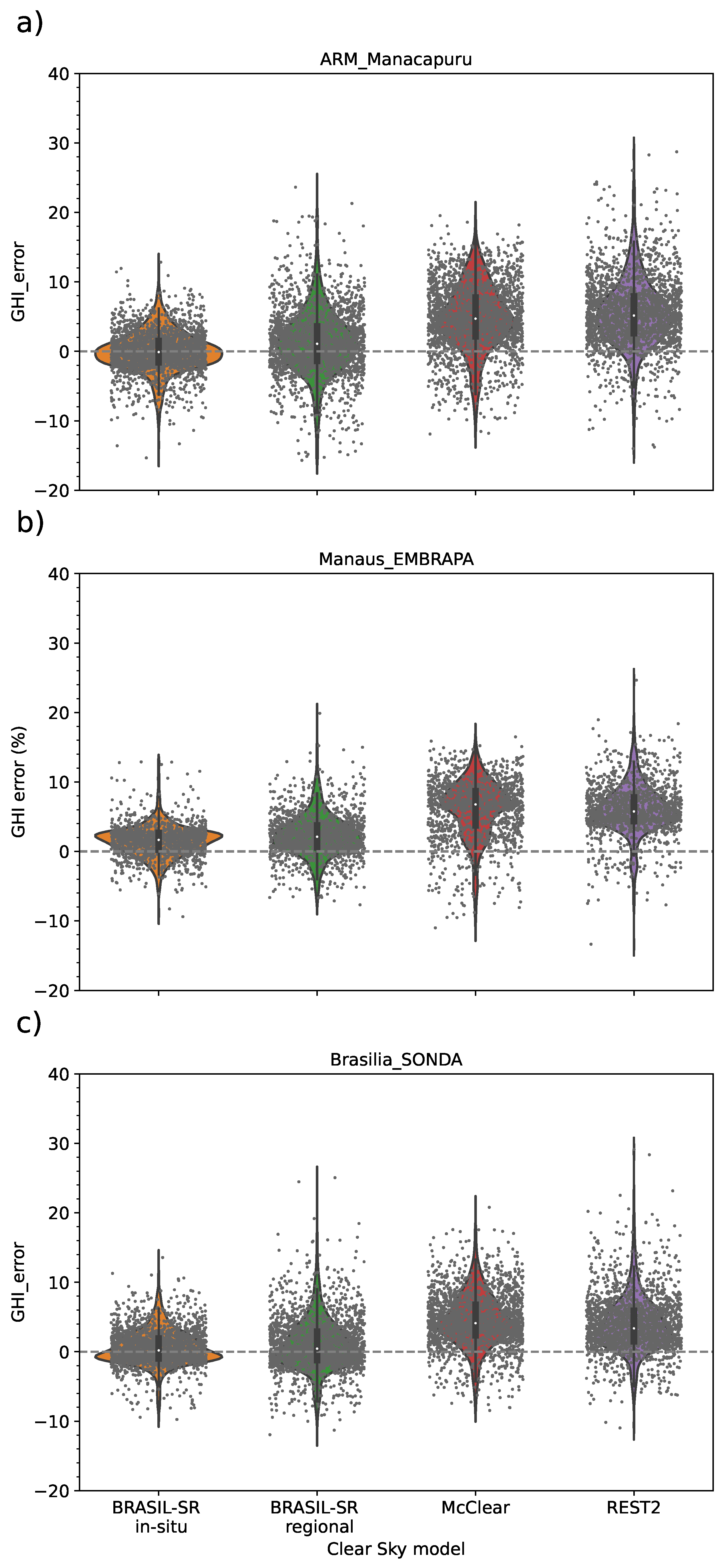
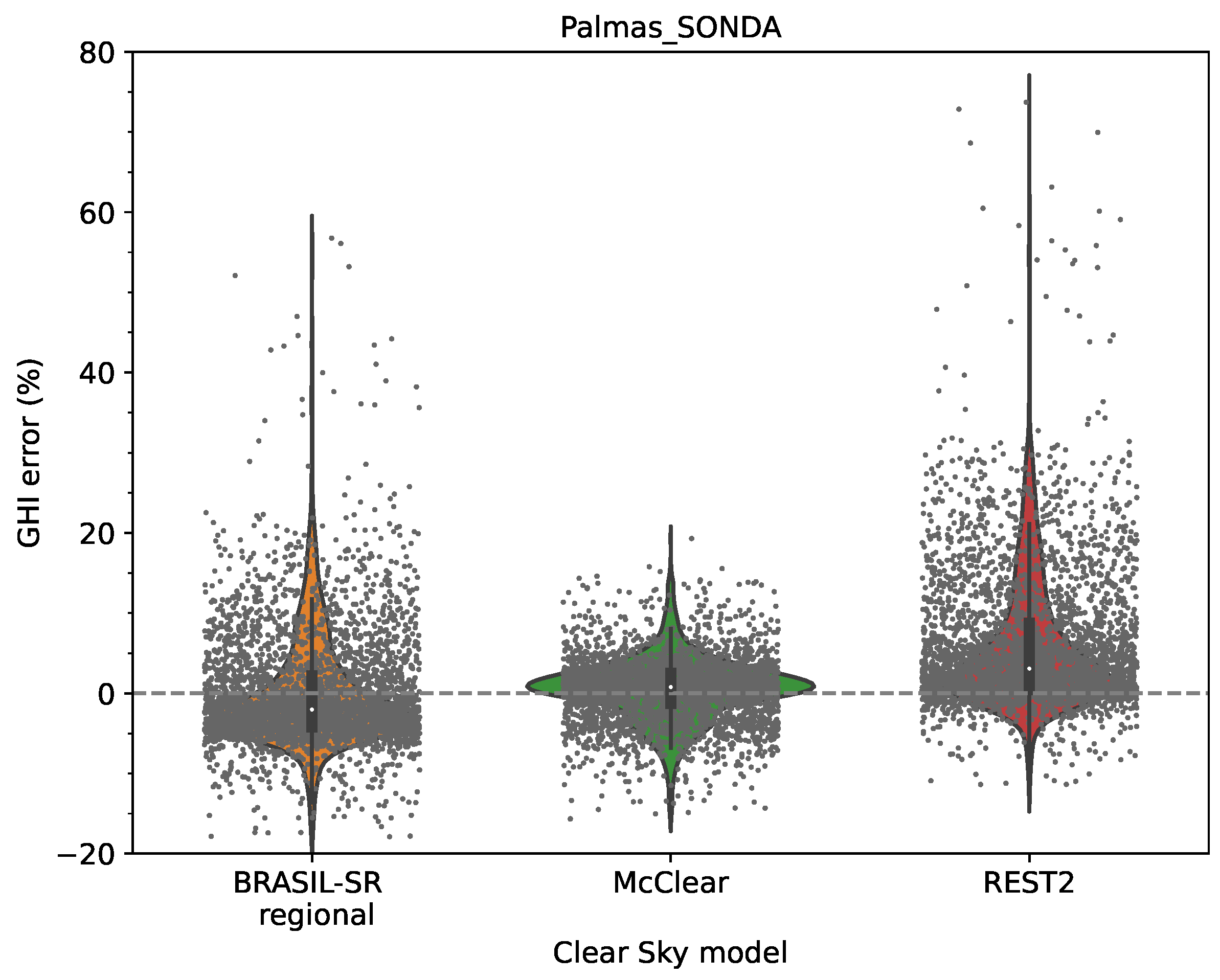
4.1. Global Horizontal Irradiation
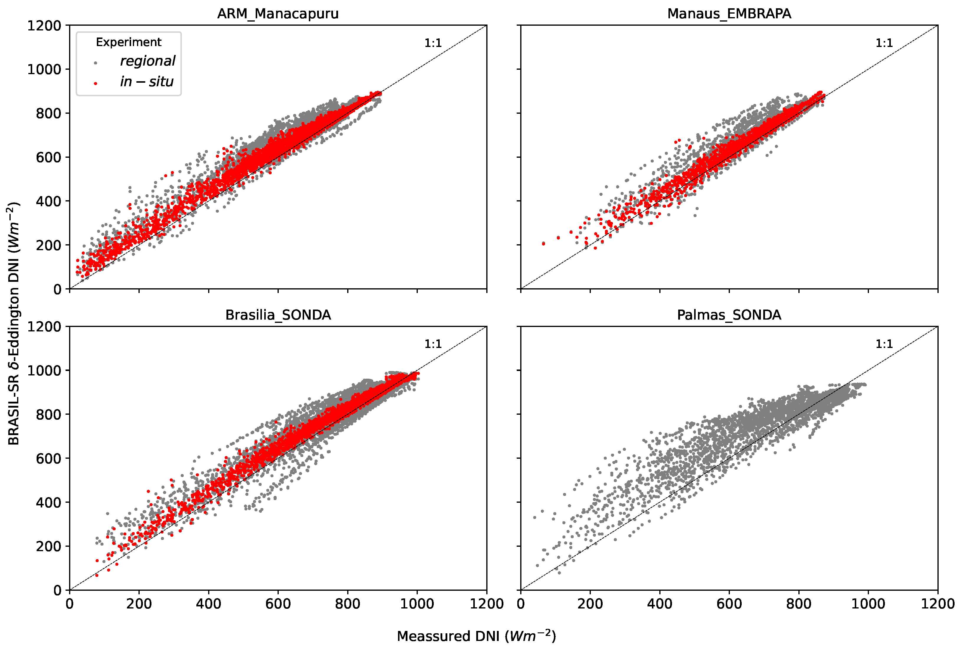
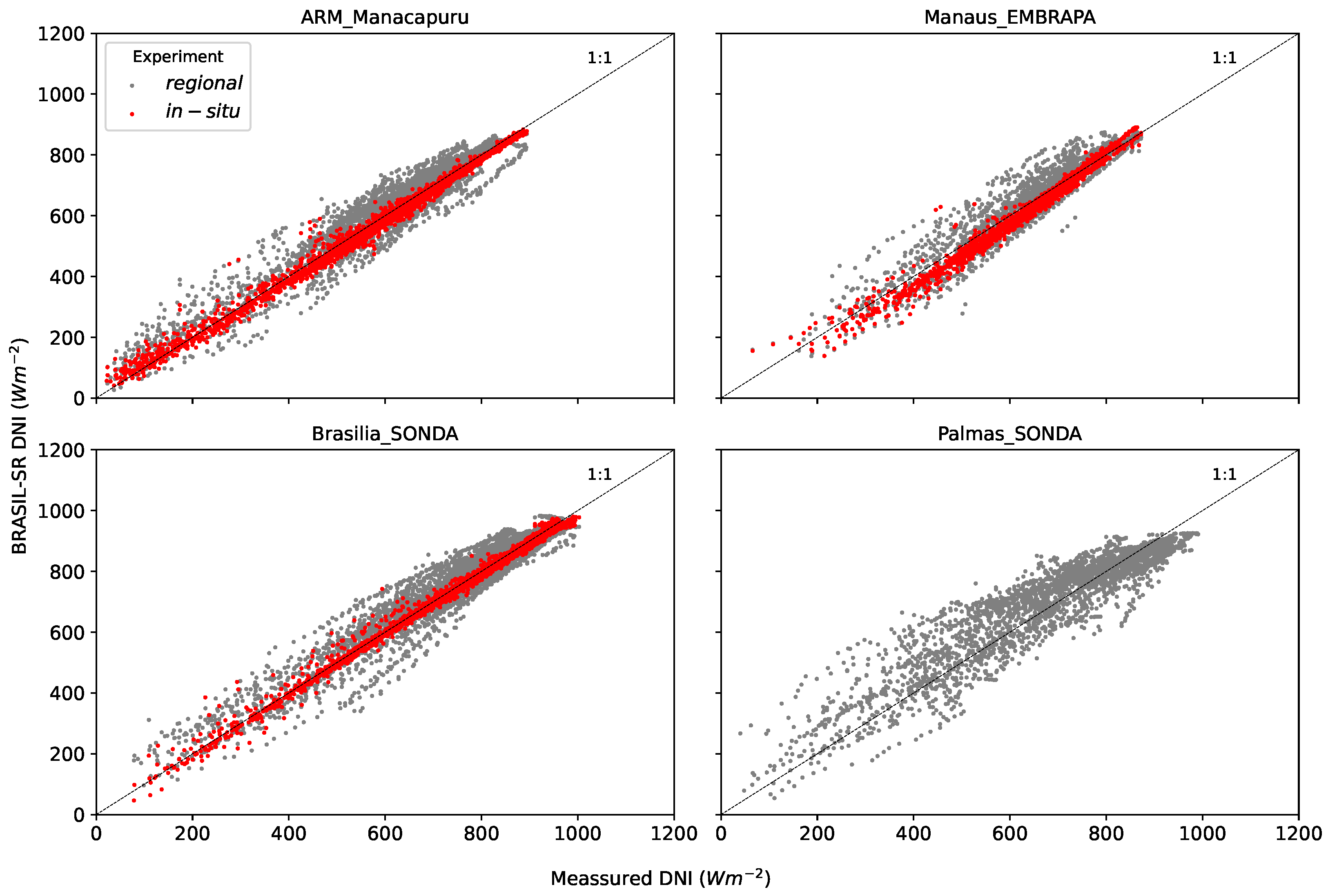
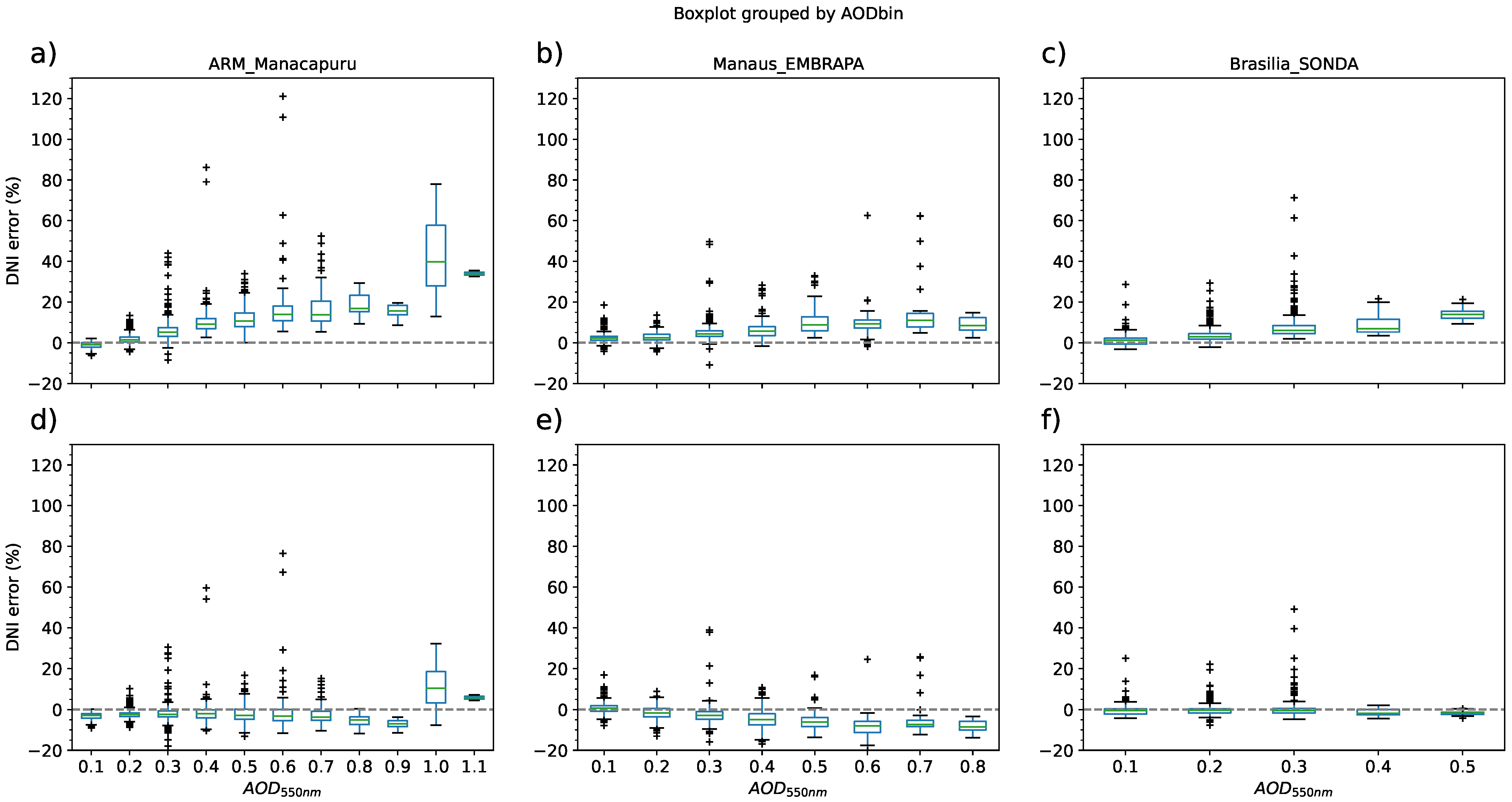
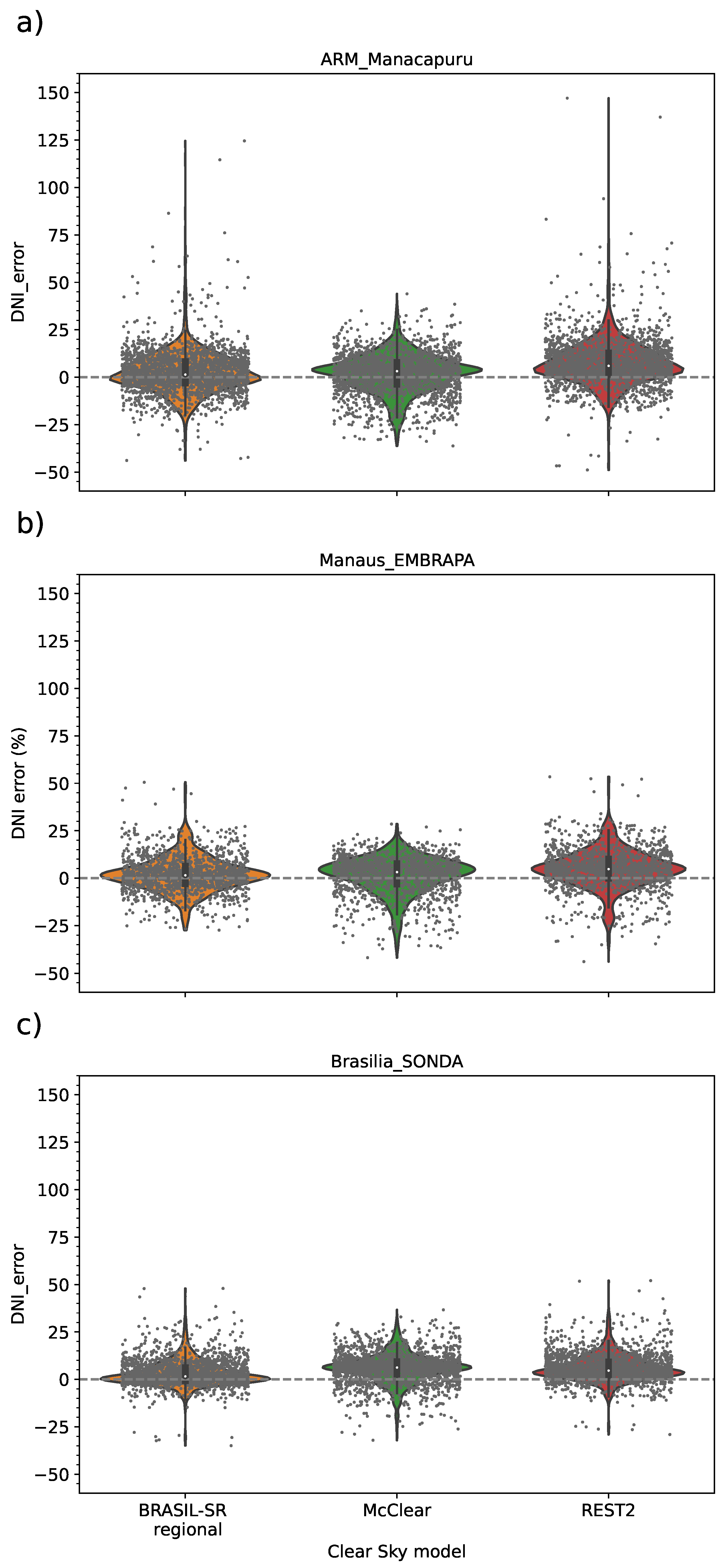
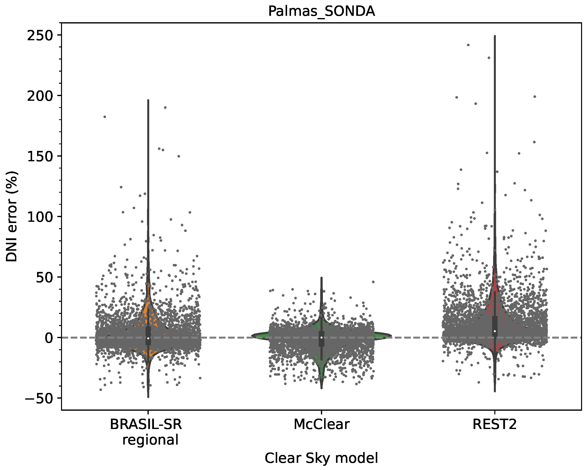
4.2. Direct Normal Irradiation
5. Discussion, Conclusions and Future Research
Author Contributions
Funding
Institutional Review Board Statement
Informed Consent Statement
Data Availability Statement
Acknowledgments
Conflicts of Interest
Abbreviations
| AERONET | Aerosol Robotic Network |
| AE | Angström’s exponent |
| AOD | Aerosol optical depth |
| ARM | Atmospheric Radiation Measurement |
| BRDF | Bi-directional reflectance distribution functions |
| BSRN | Baseline Solar Radiation Network |
| CAMS | Copernicus Atmosphere Monitoring Service |
| CS | clear-sky |
| CSP | Concentrating solar power |
| DHI | Diffuse horizontal irradiance |
| DNI | Direct (or beam) normal irradiance |
| EMBRAPA | Brazilian Agricultural Research Corporation |
| ENSO | El Niño-Southern Oscillation |
| ESFT | Exponential-sum fits to transmittances |
| GCM | General circulation models |
| GFS | Global Forecast System |
| GHI | Global horizontal irradiance |
| GOAmazon | Green Ocean Amazon |
| IBGE | Brazilian Institute of Geography and Statistics |
| IQR | Interquantile range |
| KSI | Kolmogoro-Smirnov Integral |
| MACC | Monitoring Atmospheric Composition and Climate |
| MAD | Mean absolute difference |
| MBD | Mean bias difference |
| MERRA-2 | Modern-Era Retrospective analysis for Research and Applications, Version 2 |
| MFRSR | Multifilter rotating shadowband radiometer |
| MODIS | Moderate Resolution Imaging Spectroradiometer |
| Ozone | |
| PV | Photovoltaic |
| PWV | Precipitable water vapor |
| RMSD | Root mean square difference |
| SONDA | Brazilian Environmental Data Organization System |
| SZA | Solar zenith angle |
| TOA | Top of the atmosphere |
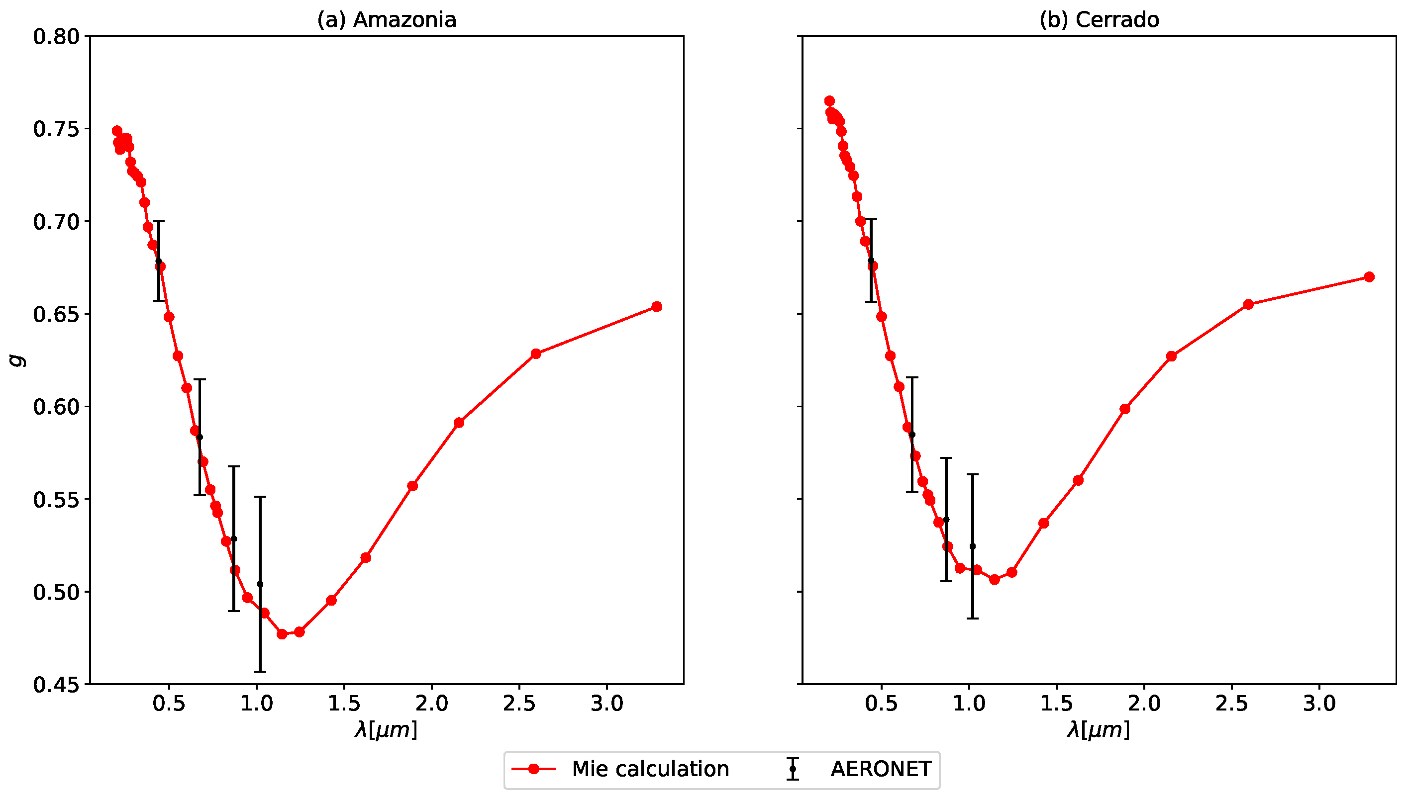
Appendix A. Biomass Burning Aerosol Optical Properties

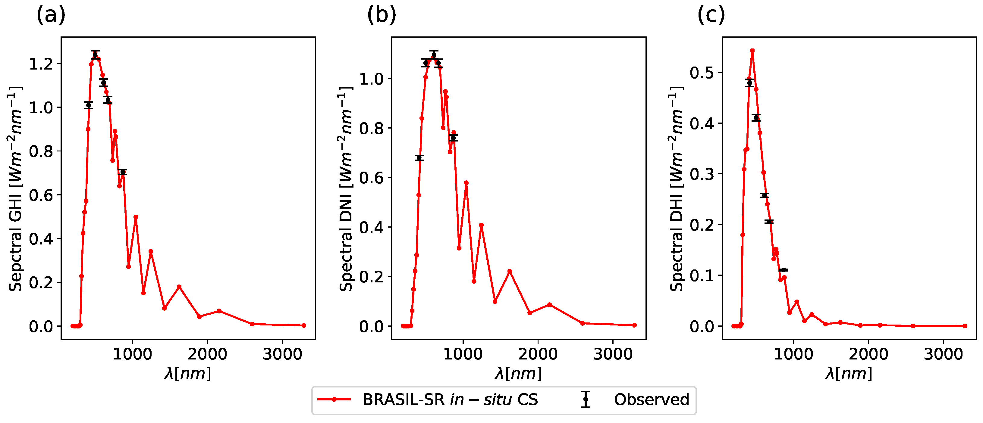
Appendix B. Spectral Irradiances with BRASIL-SR

References
- De Lima, F.J.L.; Martins, F.R.; Costa, R.S.; Gonçalves, A.R.; dos Santos, A.P.P.; Pereira, E.B. The seasonal variability and trends for the surface solar irradiation in northeastern region of Brazil. Sustain. Energy Technol. Assess. 2019, 35, 335–346. [Google Scholar] [CrossRef]
- Viana, T.; Rüther, R.; Martins, F.; Pereira, E. Assessing the potential of concentrating solar photovoltaic generation in Brazil with satellite-derived direct normal irradiation. Sol. Energy 2011, 85, 486–495. [Google Scholar] [CrossRef]
- Prăvălie, R.; Patriche, C.; Bandoc, G. Spatial assessment of solar energy potential at global scale. A geographical approach. J. Clean. Prod. 2019, 209, 692–721. [Google Scholar] [CrossRef]
- Malagueta, D.; Szklo, A.; Borba, B.S.M.C.; Soria, R.; Aragão, R.; Schaeffer, R.; Dutra, R. Assessing incentive policies for integrating centralized solar power generation in the Brazilian electric power system. Energy Policy 2013, 59, 198–212. [Google Scholar] [CrossRef]
- Dos Santos Carstens, D.D.; da Cunha, S.K. Challenges and opportunities for the growth of solar photovoltaic energy in Brazil. Energy Policy 2019, 125, 396–404. [Google Scholar] [CrossRef]
- Schmidt, J.; Cancella, R.; Pereira, A.O. The role of wind power and solar PV in reducing risks in the Brazilian hydro-thermal power system. Energy 2016, 115, 1748–1757. [Google Scholar] [CrossRef]
- Dantas, G.d.A.; de Castro, N.J.; Brandão, R.; Rosental, R.; Lafranque, A. Prospects for the Brazilian electricity sector in the 2030s: Scenarios and guidelines for its transformation. Renew. Sustain. Energy Rev. 2017, 68, 997–1007. [Google Scholar] [CrossRef]
- Luz, T.; Moura, P.; de Almeida, A. Multi-objective power generation expansion planning with high penetration of renewables. Renew. Sustain. Energy Rev. 2018, 81, 2637–2643. [Google Scholar] [CrossRef]
- de Campos, É.F.; Pereira, E.B.; van Oel, P.; Martins, F.R.; Gonçalves, A.R.; Costa, R.S. Hybrid power generation for increasing water and energy securities during drought: Exploring local and regional effects in a semi-arid basin. J. Environ. Manag. 2021, 294, 112989. [Google Scholar] [CrossRef]
- Martins, F.; Abreu, S.; Pereira, E. Scenarios for solar thermal energy applications in Brazil. Energy Policy 2012, 48, 640–649. [Google Scholar] [CrossRef]
- Soria, R.; Lucena, A.F.; Tomaschek, J.; Fichter, T.; Haasz, T.; Szklo, A.; Schaeffer, R.; Rochedo, P.; Fahl, U.; Kern, J. Modelling concentrated solar power (CSP) in the Brazilian energy system: A soft-linked model coupling approach. Energy 2016, 116, 265–280. [Google Scholar] [CrossRef]
- Fichter, T.; Soria, R.; Szklo, A.; Schaeffer, R.; Lucena, A.F. Assessing the potential role of concentrated solar power (CSP) for the northeast power system of Brazil using a detailed power system model. Energy 2017, 121, 695–715. [Google Scholar] [CrossRef]
- De Souza, L.E.V.; Cavalcante, A.M.G. Concentrated Solar Power deployment in emerging economies: The cases of China and Brazil. Renew. Sustain. Energy Rev. 2017, 72, 1094–1103. [Google Scholar] [CrossRef]
- Soria, R.; Portugal-Pereira, J.; Szklo, A.; Milani, R.; Schaeffer, R. Hybrid concentrated solar power (CSP)–biomass plants in a semiarid region: A strategy for CSP deployment in Brazil. Energy Policy 2015, 86, 57–72. [Google Scholar] [CrossRef]
- Milani, R.; Szklo, A.; Hoffmann, B.S. Hybridization of concentrated solar power with biomass gasification in Brazil’s semiarid region. Energy Convers. Manag. 2017, 143, 522–537. [Google Scholar] [CrossRef]
- Rosário, N.E.d.; Longo, K.M.; Freitas, S.R.d.; Yamasoe, M.A.; Fonseca, R.M.d. Modeling the South American regional smoke plume: Aerosol optical depth variability and surface shortwave flux perturbation. Atmos. Chem. Phys. 2013, 13, 2923–2938. [Google Scholar] [CrossRef] [Green Version]
- Martins, L.D.; Hallak, R.; Alves, R.C.; de Almeida, D.S.; Squizzato, R.; Moreira, C.A.; Beal, A.; da Silva, I.; Rudke, A.; Martins, J.A.; et al. Long-range transport of aerosols from biomass burning over southeastern South America and their implications on air quality. Aerosol Air Qual. Res. 2018, 18, 1734–1745. [Google Scholar] [CrossRef] [Green Version]
- Yamasoe, M.; Rosário, N.; Barros, K. Downward solar global irradiance at the surface in São Paulo city—The climatological effects of aerosol and clouds. J. Geophys. Res. Atmos. 2017, 122, 391–404. [Google Scholar] [CrossRef]
- Jury, M.R.; Pabón, A.R. Dispersion of smoke plumes over South America. Earth Interact. 2021, 25, 1–14. [Google Scholar] [CrossRef]
- Gueymard, C.A. Temporal variability in direct and global irradiance at various time scales as affected by aerosols. Sol. Energy 2012, 86, 3544–3553. [Google Scholar] [CrossRef]
- Gueymard, C.A.; Ruiz-Arias, J.A. Validation of direct normal irradiance predictions under arid conditions: A review of radiative models and their turbidity-dependent performance. Renew. Sustain. Energy Rev. 2015, 45, 379–396. [Google Scholar] [CrossRef]
- Ruiz-Arias, J.A.; Gueymard, C.A.; Cebecauer, T. Direct normal irradiance modeling: Evaluating the impact on accuracy of worldwide gridded aerosol databases. AIP Conf. Proc. 2019, 2126, 190013. [Google Scholar] [CrossRef]
- Boraiy, M.; Korany, M.; Aoun, Y.; Alfaro, S.C.; El-Metwally, M.; Abdelwahab, M.M.; Blanc, P.; Eissa, Y.; Ghedira, H.; Siour, G.; et al. Improving direct normal irradiance retrieval in cloud-free, but high aerosol load conditions by using aerosol optical depth. Meteorol. Z. 2017, 26, 475–483. [Google Scholar] [CrossRef]
- Artaxo, P.; Rizzo, L.V.; Brito, J.F.; Barbosa, H.M.; Arana, A.; Sena, E.T.; Cirino, G.G.; Bastos, W.; Martin, S.T.; Andreae, M.O. Atmospheric aerosols in Amazonia and land use change: From natural biogenic to biomass burning conditions. Faraday Discuss. 2013, 165, 203–235. [Google Scholar] [CrossRef] [PubMed] [Green Version]
- Sengupta, M.; Habte, A.; Wilbert, S.; Gueymard, C.; Remund, J. Best Practices Handbook for the Collection and Use of Solar Resource Data for Solar Energy Applications, 3rd ed.; NREL: Golden, CO, USA, 2021; pp. 1–348.
- Pereira, E.B.; Martins, F.R.; de Abreu, S.L.; Rüther, R. Atlas Brasileiro de Energia Solar; INPE: São José dos Campos, Brazil, 2006; Volume 1.
- Martins, F.R.; Gonçalves, A.R.; Costa, R.S.; Lima, F.L.; Rüther, R.; Abreu, S.L.; Tiepolo, G.M.; Pereira, S.V.; Souza, J.G. Atlas Brasileiro de Energia Solar, 2nd ed.; INPE: São José dos Campos, Brazil, 2017; p. 88.
- Martins, F.; Pereira, E.B. Parameterization of aerosols from burning biomass in the Brazil-SR radiative transfer model. Sol. Energy 2006, 80, 231–239. [Google Scholar] [CrossRef]
- Martins, F.; Pereira, E.; Silva, S.; Abreu, S.; Colle, S. Solar energy scenarios in Brazil, Part one: Resource assessment. Energy Policy 2008, 36, 2853–2864. [Google Scholar] [CrossRef]
- Costa, R.S.; Martins, F.R.; Pereira, E.B. Atmospheric aerosol influence on the Brazilian solar energy assessment: Experiments with different horizontal visibility bases in radiative transfer model. Renew. Energy 2016, 90, 120–135. [Google Scholar] [CrossRef]
- Landulfo, E.; Lopes, F.J. Initial approach in biomass burning aerosol transport tracking with CALIPSO and MODIS satellites, sunphotometer, and a backscatter lidar system in Brazil. In Proceedings of the Lidar Technologies, Techniques, and Measurements for Atmospheric Remote Sensing V. International Society for Optics and Photonics, Berlin, Germany, 31 August–3 September 2009; Volume 7479, pp. 40–48. [Google Scholar]
- Darbyshire, E.; Morgan, W.T.; Allan, J.D.; Liu, D.; Flynn, M.J.; Dorsey, J.R.; O´Shea, S.J.; Lowe, D.; Szpek, K.; Marenco, F.; et al. The vertical distribution of biomass burning pollution over tropical South America from aircraft in situ measurements during SAMBBA. Atmos. Chem. Phys. Discuss. 2018, 19, 5771–5790. [Google Scholar] [CrossRef] [Green Version]
- Holben, B.; Eck, T.; Slutsker, I.; Tanré, D.; Buis, J.; Setzer, A.; Vermote, E.; Reagan, J.; Kaufman, Y.; Nakajima, T.; et al. AERONET—A Federated Instrument Network and Data Archive for Aerosol Characterization. Remote Sens. Environ. 1998, 66, 1–16. [Google Scholar] [CrossRef]
- Wiscombe, W.J.; Evans, J.W. Exponential-sum fitting of radiative transmission functions. J. Comput. Phys. 1977, 24, 416–444. [Google Scholar] [CrossRef]
- Schreier, F.; García, S.G.; Hochstaffl, P.; Städt, S. Py4CAtS-PYthon for computational ATmospheric spectroscopy. Atmosphere 2019, 10, 262. [Google Scholar] [CrossRef] [Green Version]
- Gordon, I.E.; Rothman, L.S.; Hill, C.; Kochanov, R.V.; Tan, Y.; Bernath, P.F.; Birk, M.; Boudon, V.; Campargue, A.; Chance, K.; et al. The HITRAN2016 molecular spectroscopic database. J. Quant. Spectrosc. Radiat. Transf. 2017, 203, 3–69. [Google Scholar] [CrossRef]
- Gueymard, C. The sun’s total and spectral irradiance for solar energy applications and solar radiation models. Sol. Energy 2004, 76, 423–453. [Google Scholar] [CrossRef]
- Anderson, G.P.; Clough, S.A.; Kneizys, F.X.; Chetwynd, J.H., Jr.; Shettle, E.P. Atmospheric Constituent Profiles (0–120 km); Technical Report AFGL-TR-86-0110; Air Force Geophysical Laboratory: Hanscom AFB, MA, USA, 1986. [Google Scholar]
- Schaaf, C.B.; Gao, F.; Strahler, A.H.; Lucht, W.; Li, X.; Tsang, T.; Strugnell, N.C.; Zhang, X.; Jin, Y.; Muller, J.P.; et al. First operational BRDF, albedo nadir reflectance products from MODIS. Remote Sens. Environ. 2002, 83, 135–148. [Google Scholar] [CrossRef] [Green Version]
- Emde, C.; Buras-Schnell, R.; Kylling, A.; Mayer, B.; Gasteiger, J.; Hamann, U.; Kylling, J.; Richter, B.; Pause, C.; Dowling, T.; et al. The libRadtran software package for radiative transfer calculations (version 2.0.1). Geosci. Model Dev. 2016, 9, 1647–1672. [Google Scholar] [CrossRef] [Green Version]
- Laszlo, I.; Stamnes, K.; Wiscombe, W.J.; Tsay, S.C. The discrete ordinate algorithm, DISORT for radiative transfer. In Light Scattering Reviews; Springer: Berlin/Heidelberg, Germany, 2016; Volume 11, pp. 3–65. [Google Scholar]
- Martin, S.T.; Artaxo, P.; Machado, L.A.T.; Manzi, A.O.; Souza, R.A.F.d.; Schumacher, C.; Wang, J.; Andreae, M.O.; Barbosa, H.; Fan, J.; et al. Introduction: Observations and modeling of the Green Ocean Amazon (GoAmazon2014/5). Atmos. Chem. Phys. 2016, 16, 4785–4797. [Google Scholar] [CrossRef] [Green Version]
- Jiménez-Muñoz, J.C.; Mattar, C.; Barichivich, J.; Santamaría-Artigas, A.; Takahashi, K.; Malhi, Y.; Sobrino, J.A.; Van Der Schrier, G. Record-breaking warming and extreme drought in the Amazon rainforest during the course of El Niño 2015–2016. Sci. Rep. 2016, 6, 1–7. [Google Scholar] [CrossRef] [Green Version]
- Aragão, L.E.; Anderson, L.O.; Fonseca, M.G.; Rosan, T.M.; Vedovato, L.B.; Wagner, F.H.; Silva, C.V.; Silva Junior, C.H.; Arai, E.; Aguiar, A.P.; et al. 21st Century drought-related fires counteract the decline of Amazon deforestation carbon emissions. Nat. Commun. 2018, 9, 536. [Google Scholar] [CrossRef]
- Silva Junior, C.H.; Anderson, L.O.; Silva, A.L.; Almeida, C.T.; Dalagnol, R.; Pletsch, M.A.; Penha, T.V.; Paloschi, R.A.; Aragão, L.E. Fire responses to the 2010 and 2015/2016 Amazonian droughts. Front. Earth Sci. 2019, 7, 97. [Google Scholar] [CrossRef]
- Barbosa, H.d.M.J.; Barja, B.; Pauliquevis, T.; Gouveia, D.A.; Artaxo, P.; Cirino, G.; Santos, R.; Oliveira, A. A permanent Raman lidar station in the Amazon: Description, characterization, and first results. Atmos. Meas. Tech. 2014, 7, 1745–1762. [Google Scholar] [CrossRef] [Green Version]
- da Silva, P.E.D.; Martins, F.R.; Pereira, E.B. Quality Control of Solar Radiation Data within Sonda Network in Brazil: Preliminary results. In Proceedings of the EUROSUN 2014, Aux-les-Bains, France, 16–19 September 2014. [Google Scholar]
- Sistema de Organização Nacional de Dados Ambientais. 2021. Available online: http://sonda.ccst.inpe.br/index.html (accessed on 15 May 2020).
- Andreas, A.; Dooraghi, M.; Habte, A.; Kutchenreiter, M.; Reda, I.; Sengupta, M. Solar Infrared Radiation Station (SIRS), Sky Radiation (SKYRAD), Ground Radiation (GNDRAD), and Broadband Radiometer Station (BRS) Instrument Handbook; U.S. Department of Energy, ARM Climate Reaearch Facility Technical Report DOE/SC-ARM-TR-025; U.S. Department of Energy: Washington, DC, USA, 2018.
- Atmospheric Radiation Measurement (ARM) User Facility. MFRSR: Derived AOD Using the First Michalsky Algorithm (MFRSRAOD1MICH); ARM Mobile Facility (MAO) Manacapuru: Amazonas, Brazil, 2014. [CrossRef]
- Atmospheric Radiation Measurement (ARM) User Facility. Sky Radiometers on Stand for Downwelling Radiation (SKYRAD60S); Sengupta, M., Andreas, A., Dooraghi, M., Habte, A., Kutchenreiter, M., Reda, I., Morris, V., Xie, Y., Gotseff, P., Eds.; ARM Mobile Facility (MAO) Manacapuru: Amazonas, Brazil, 2014. [CrossRef]
- Baseline Surface Radiation Network. 2021. Available online: https://bsrn.awi.de/ (accessed on 10 May 2021).
- Rosário, N.E.; Sauini, T.; Pauliquevis, T.; Barbosa, H.M.; Yamasoe, M.A.; Barja, B. Aerosol optical depth retrievals in central Amazonia from a multi-filter rotating shadow-band radiometer calibrated on-site. Atmos. Meas. Tech. 2019, 12, 921–934. [Google Scholar] [CrossRef] [Green Version]
- Roesch, A.; Wild, M.; Ohmura, A.; Dutton, E.G.; Long, C.N.; Zhang, T. Assessment of BSRN radiation records for the computation of monthly means. Atmos. Meas. Tech. 2011, 4, 339–354. [Google Scholar] [CrossRef] [Green Version]
- Lefèvre, M.; Oumbe, A.; Blanc, P.; Espinar, B.; Gschwind, B.; Qu, Z.; Wald, L.; Schroedter-Homscheidt, M.; Hoyer-Klick, C.; Arola, A.; et al. McClear: A new model estimating downwelling solar radiation at ground level in clear-sky conditions. Atmos. Meas. Tech. 2013, 6, 2403–2418. [Google Scholar] [CrossRef] [Green Version]
- Blanc, P.; Gschwind, B.; Ménard, L.; Wald, L.; Tournadre, B. MODIS-Derived Surface BRDF for Land and Water Masses; MINES ParisTech: Paris, France, 2017. [Google Scholar] [CrossRef]
- IBGE. Biomes of Brazil. Available online: https://www.ibge.gov.br/en/geosciences/maps/brazil-environmental-information/18341-biomes.html?=&t=acesso-ao-produto (accessed on 20 January 2021).
- Randles, C.; Da Silva, A.; Buchard, V.; Colarco, P.; Darmenov, A.; Govindaraju, R.; Smirnov, A.; Holben, B.; Ferrare, R.; Hair, J.; et al. The MERRA-2 aerosol reanalysis, 1980 onward. Part I: System description and data assimilation evaluation. J. Clim. 2017, 30, 6823–6850. [Google Scholar] [CrossRef]
- Buchard, V.; Randles, C.; Da Silva, A.; Darmenov, A.; Colarco, P.; Govindaraju, R.; Ferrare, R.; Hair, J.; Beyersdorf, A.; Ziemba, L.; et al. The MERRA-2 aerosol reanalysis, 1980 onward. Part II: Evaluation and case studies. J. Clim. 2017, 30, 6851–6872. [Google Scholar] [CrossRef] [PubMed]
- Copernicus Climate Change Service. Ozone Monthly Gridded Data from 1970 to Present Derived from Satellite Observations. 2021. Available online: https://cds.climate.copernicus.eu/cdsapp#!/dataset/10.24381/cds.4ebfe4eb?tab=overview (accessed on 10 February 2021).
- National Centers for Environmental Prediction; National Weather Service, NOAA, U.S. NCEP GFS 0.25 Degree Global Forecast Grids Historical Archive; Research Data Archive at the National Center for Atmospheric Research, Computational and Information Systems Laboratory, Boulder, Colorado; National Centers for Environmental Prediction: College Park, MD, USA, 2015.
- Gueymard, C.A. A review of validation methodologies and statistical performance indicators for modeled solar radiation data: Towards a better bankability of solar projects. Renew. Sustain. Energy Rev. 2014, 39, 1024–1034. [Google Scholar] [CrossRef]
- Gschwind, B.; Wald, L.; Blanc, P.; Lefèvre, M.; Schroedter-Homscheidt, M.; Arola, A. Improving the McClear model estimating the downwelling solar radiation at ground level in cloud-free conditions–McClear-v3. Meteorol. Z. 2019, 28, 147–163. [Google Scholar] [CrossRef]
- Gueymard, C.A. REST2: High-performance solar radiation model for cloudless-sky irradiance, illuminance, and photosynthetically active radiation–Validation with a benchmark dataset. Sol. Energy 2008, 82, 272–285. [Google Scholar] [CrossRef]
- Bright, J.M.; Bai, X.; Zhang, Y.; Sun, X.; Acord, B.; Wang, P. irradpy: Python package for MERRA-2 download, extraction and usage for clear-sky irradiance modelling. Sol. Energy 2020, 199, 685–693. [Google Scholar] [CrossRef]
- Copernicus Atmosphere Monitoring Service. CAMS McClear Service for Irradiation under Clear-Sky. 2021. Available online: http://www.soda-pro.com/web-services/radiation/cams-mcclear (accessed on 25 July 2021).
- Myers, D.R.; Gueymard, C.A. Description and availability of the SMARTS spectral model for photovoltaic applications. In Proceedings of the Organic Photovoltaics V. International Society for Optics and Photonics, Denver, CO, USA, 2–6 August 2004; Volume 5520, pp. 56–67. [Google Scholar]
- Bright, J.M.; Sun, X.; Gueymard, C.A.; Acord, B.; Wang, P.; Engerer, N.A. BRIGHT-SUN: A globally applicable 1-min irradiance clear-sky detection model. Renew. Sustain. Energy Rev. 2020, 121, 109706. [Google Scholar] [CrossRef]
- Inman, R.H.; Edson, J.G.; Coimbra, C.F. Impact of local broadband turbidity estimation on forecasting of clear sky direct normal irradiance. Sol. Energy 2015, 117, 125–138. [Google Scholar] [CrossRef] [Green Version]
- Ineichen, P. Comparison of eight clear sky broadband models against 16 independent data banks. Sol. Energy 2006, 80, 468–478. [Google Scholar] [CrossRef] [Green Version]
- Ineichen, P.; Barroso, C.S.; Geiger, B.; Hollmann, R.; Marsouin, A.; Mueller, R. Satellite Application Facilities irradiance products: Hourly time step comparison and validation over Europe. Int. J. Remote Sens. 2009, 30, 5549–5571. [Google Scholar] [CrossRef]
- Gueymard, C.A.; Bright, J.M.; Lingfors, D.; Habte, A.; Sengupta, M. A posteriori clear-sky identification methods in solar irradiance time series: Review and preliminary validation using sky imagers. Renew. Sustain. Energy Rev. 2019, 109, 412–427. [Google Scholar] [CrossRef]
- Bright, J.M. Clear-Sky Detection Library. Github Repository. 2018. Available online: https://github.com/JamieMBright/csd-library (accessed on 14 June 2021).
- Reno, M.J.; Hansen, C.W.; Stein, J.S. Global Horizontal Irradiance Clear Sky Models: Implementation and Analysis; SANDIA Report SAND2012-2389; Sandia National Laboratories (SNL): Albuquerque, NM, USA; Livermore, CA, USA, 2012.
- Shi, G.; Sun, Z.; Li, J.; He, Y. Fast scheme for determination of direct normal irradiance. Part I: New aerosol parameterization and performance assessment. Sol. Energy 2020, 199, 268–277. [Google Scholar] [CrossRef]
- Joseph, J.H.; Wiscombe, W.; Weinman, J. The delta-Eddington approximation for radiative flux transfer. J. Atmos. Sci. 1976, 33, 2452–2459. [Google Scholar] [CrossRef]
- Gueymard, C.A. Aerosol turbidity derivation from broadband irradiance measurements: Methodological advances and uncertainty analysis. In Proceedings of the 42nd ASES National Solar Conference 2013, SOLAR 2013, Including 42nd ASES Annual Conference and 38th National Passive Solar Conference, Baltimore, MD, USA, 16–20 April 2013; pp. 637–644. [Google Scholar]
- Sun, Z.; Li, J.; He, Y.; Li, J.; Liu, A.; Zhang, F. Determination of direct normal irradiance including circumsolar radiation in climate/NWP models. Q. J. R. Meteorol. Soc. 2016, 142, 2591–2598. [Google Scholar] [CrossRef]
- Räisänen, P.; Lindfors, A.V. On the computation of apparent direct solar radiation. J. Atmos. Sci. 2019, 76, 2761–2780. [Google Scholar] [CrossRef]
- Gueymard, C.A. Parameterized transmittance model for direct beam and circumsolar spectral irradiance. Sol. Energy 2001, 71, 325–346. [Google Scholar] [CrossRef]
- AErosol RObotic NETwork. 2021. Available online: http://https://aeronet.gsfc.nasa.gov/ (accessed on 21 November 2019).
- Eck, T.F.; Holben, B.N.; Reid, J.S.; Dubovik, O.; Smirnov, A.; O’Neill, N.T.; Slutsker, I.; Kinne, S. Wavelength dependence of the optical depth of biomass burning, urban, and desert dust aerosols. J. Geophys. Res. Atmos. 1999, 104, 31333–31349. [Google Scholar] [CrossRef]
- Schafer, J.S.; Eck, T.F.; Holben, B.N.; Artaxo, P.; Duarte, A.F. Characterization of the optical properties of atmospheric aerosols in Amazônia from long-term AERONET monitoring (1993–1995 and 1999–2006). J. Geophys. Res. Atmos. 2008, 113, 1–16. [Google Scholar] [CrossRef] [Green Version]
- Giles, D.M.; Holben, B.N.; Eck, T.F.; Sinyuk, A.; Smirnov, A.; Slutsker, I.; Dickerson, R.R.; Thompson, A.M.; Schafer, J.S. An analysis of AERONET aerosol absorption properties and classifications representative of aerosol source regions. J. Geophys. Res. Atmos. 2012, 117, 1–16. [Google Scholar] [CrossRef] [Green Version]
- Pérez-Ramírez, D.; Andrade-Flores, M.; Eck, T.F.; Stein, A.F.; O’Neill, N.T.; Lyamani, H.; Gassó, S.; Whiteman, D.N.; Veselovskii, I.; Velarde, F.; et al. Multi year aerosol characterization in the tropical Andes and in adjacent Amazonia using AERONET measurements. Atmos. Environ. 2017, 166, 412–432. [Google Scholar] [CrossRef] [Green Version]
- Virtanen, P.; Gommers, R.; Oliphant, T.E.; Haberland, M.; Reddy, T.; Cournapeau, D.; Burovski, E.; Peterson, P.; Weckesser, W.; Bright, J.; et al. SciPy 1.0: Fundamental algorithms for scientific computing in Python. Nat. Methods 2020, 17, 261–272. [Google Scholar] [CrossRef] [Green Version]
- Wiscombe, W.J. Mie Scattering Calculations: Advances in Technique and Fast, Vector-Speed Computer Codes; Technical Note NCAR/TN-140+STR; National Center for Atmospheric Research: Boulder, CO, USA, 1979. [Google Scholar]


| Site | Latitude (°) | Longitude (°) | Variables and Instruments |
|---|---|---|---|
| ARM_Manacapuru | −3.213 | −60.598 | DNI, GHI, DHI: SKYRAD |
| Spectral irradiance, AOD, AE: MFRSR | |||
| AOD, PWV, : AERONET | |||
| Manaus_EMBRAPA | −2.891 | −59.970 | DNI, GHI, DHI, Spectral irradiance, AOD, AE: MFRSR |
| AOD, AE, PWV, : AERONET | |||
| Brasilia_SONDA | −15.601 | −47.713 | DNI: Pyrheliometer NIP Eppley/CHP 1 Kipp&Zonen |
| GHI: Pyranometer CM22 Kipp&Zonen | |||
| DHI: Pyranometer CM22 Kipp&Zonen | |||
| plus Sun tracker A2P BD | |||
| AOD, PWV, : AERONET | |||
| Palmas_SONDA | −10.179 | −48.362 | GHI: Pyranometer CM11 Kipp&Zonen |
| DHI: Pyranometer CM11 Kipp&Zonen | |||
| with shadowing ring CM121B + adapter CV2 |
| Site | Number of Data Records | Clear-Sky/Clear-Sun | Clear-Sun | ||
|---|---|---|---|---|---|
| Bright-Sun (%) | Inman15 (%) | Ineichen06 (%) | Ineichen09 (%) | ||
| ARM_Manacapuru | 92,274 | 16.7 | 23.5 | 25.7 | 47.7 |
| Manaus_EMBRAPA | 86,218 | 12.6 | 20.7 | 25.7 | 47.1 |
| Brasilia_SONDA | 88,169 | 31.7 | 42.8 | 48.1 | 68.1 |
| Palmas_SONDA | 91,233 | 17.6 | 33.3 | 37.6 | 54.1 |
| Site | N | MBD (%) | RMSD (%) | MAD (%) | KSI % | OVER % | |
|---|---|---|---|---|---|---|---|
| BRASIL-SR In-situ | |||||||
| ARM_Manacapuru | 2758 | 460.4 | −1.2 (−0.3) | 13.4 (2.9) | 9.7 (2.1) | 14.1 | 0.0 |
| Manaus_EMBRAPA | 1631 | 459.6 | 5.9 (1.3) | 11.0 (2.4) | 9.0 (2.0) | 12.1 | 0.0 |
| Brasilia_SONDA | 2424 | 621.5 | 0.9 (0.1) | 13.0 (2.1) | 10.0 (1.6) | 14.3 | 0.0 |
| BRASIL-SR Regional | |||||||
| ARM_Manacapuru | 3088 | 461.5 | 3.3 (0.7) | 18.8 (4.1) | 14.1 (3.1) | 18.1 | 0.0 |
| Manaus_EMBRAPA | 2047 | 459.2 | 9.6 (2.1) | 15.3 (3.3) | 12.1 (2.6) | 22.6 | 0.0 |
| Brasilia_SONDA | 5742 | 582.9 | −5.1 (−0.9) | 18.5 (3.2) | 14.9 (2.6) | 21.4 | 0.0 |
| Palmas_SONDA | 3639 | 650.8 | −6.2 (−1.0) | 37.0 (5.7) | 28.9 (4.4) | 32.0 | 1.9 |
| McClear | |||||||
| ARM_Manacapuru | 3088 | 461.5 | 20.1 (4.4) | 28.6 (6.2) | 23.9 (5.2) | 57.6 | 4.5 |
| Manaus_EMBRAPA | 2047 | 459.2 | 27.3 (5.9) | 33.8 (7.4) | 29.1 (6.3) | 64.0 | 10.6 |
| Brasilia_SONDA | 5742 | 582.9 | 20.4 (3.5) | 27.4 (4.7) | 22.7 (3.9) | 79.4 | 14.9 |
| Palmas_SONDA | 3639 | 650.8 | 2.2 (0.3) | 23.1 (3.5) | 16.8 (2.6) | 9.2 | 0.0 |
| REST2 | |||||||
| ARM_Manacapuru | 3088 | 461.5 | 20.5 (4.5) | 29.7 (6.4) | 25.2 (5.5) | 91.5 | 23.7 |
| Manaus_EMBRAPA | 2047 | 459.2 | 26.6 (5.8) | 31.1 (6.8) | 27.5 (6.0) | 61.8 | 7.2 |
| Brasilia_SONDA | 5742 | 582.9 | 9.6 (1.6) | 22.7 (3.9) | 16.8 (2.9) | 54.6 | 1.0 |
| Palmas_SONDA | 3639 | 650.8 | 30.8 (4.7) | 50.7 (7.8) | 35.0 (5.4) | 97.0 | 28.6 |
| Site | N | MBD (%) | RMSD (%) | MAD (%) | KSI % | OVER % | |
|---|---|---|---|---|---|---|---|
| In-situ | |||||||
| ARM_Manacapuru | 2758 | 575.9 | 31.1 (5.4) | 44.6 (7.7) | 34.8 (6.0) | 83.8 | 29.8 |
| Manaus_EMBRAPA | 1631 | 628.5 | 25.2 (4.0) | 34.9 (5.5) | 27.8 (4.4) | 52.3 | 14.7 |
| Brasilia_SONDA | 2424 | 744.5 | 30.9 (4.1) | 39.5 (5.3) | 32.3 (4.3) | 78.7 | 27.3 |
| Regional | |||||||
| ARM_Manacapuru | 3088 | 584.4 | 49.0 (8.4) | 72.1 (12.3) | 56.9 (9.7) | 140.3 | 76.9 |
| Manaus_EMBRAPA | 2047 | 631.7 | 40.6 (6.4) | 64.7 (10.2) | 50.9 (8.1) | 94.5 | 51.3 |
| Brasilia_SONDA | 5742 | 775.8 | 19.4 (2.5) | 56.0 (7.2) | 40.5 (5.2) | 76.2 | 30.1 |
| Palmas_SONDA | 3639 | 715.8 | 40.9 (5.7) | 89.3 (12.5) | 64.3 (9.0) | 153.5 | 91.9 |
| Site | N | MBD (%) | RMSD (%) | MAD (%) | KSI (%) | OVER (%) | |
|---|---|---|---|---|---|---|---|
| In-situ | |||||||
| ARM_Manacapuru | 2758 | 575.9 | −13.4 (−2.3) | 24.7 (4.3) | 20.0 (3.5) | 41.0 | 5.3 |
| Manaus_EMBRAPA | 1631 | 628.5 | −13.7 (−2.2) | 29.3 (4.7) | 22.8 (3.6) | 35.6 | 1.5 |
| Brasilia_SONDA | 2424 | 744.5 | −4.1 (−0.5) | 17.2 (2.3) | 11.7 (1.6) | 12.3 | 0.0 |
| Regional | |||||||
| ARM_Manacapuru | 3088 | 584.4 | 12.1 (2.1) | 53.4 (9.1) | 42.4 (7.3) | 35.8 | 1.7 |
| Manaus_EMBRAPA | 2047 | 631.7 | 9.0 (1.4) | 51.0 (8.1) | 39.3 (6.2) | 28.8 | 6.2 |
| Brasilia_SONDA | 5742 | 775.8 | 0.8 (0.1) | 45.8 (5.9) | 33.0 (4.3) | 25.1 | 1.6 |
| Palmas_SONDA | 3639 | 715.8 | 8.1 (1.1) | 68.7 (9.6) | 51.4 (7.2) | 79.7 | 26.9 |
| McClear | |||||||
| ARM_Manacapuru | 3088 | 584.4 | 10.5 (1.8) | 57.3 (9.8) | 45.9 (7.9) | 47.9 | 15.7 |
| Manaus_EMBRAPA | 2047 | 631.7 | 9.8 (1.6) | 57.2 (9.0) | 45.9 (7.3) | 65.3 | 22.5 |
| Brasilia_SONDA | 5742 | 775.8 | 35.9 (4.6) | 59.9 (7.7) | 50.3 (6.5) | 140.1 | 99.9 |
| Palmas_SONDA | 3639 | 715.8 | −7.4 (−1.0) | 52.5 (7.3) | 39.3 (5.5) | 48.3 | 6.4 |
| REST2 | |||||||
| ARM_Manacapuru | 3088 | 584.4 | 40.5 (6.9) | 66.9 (11.4) | 54.3 (9.3) | 116.1 | 60.0 |
| Manaus_EMBRAPA | 2047 | 631.7 | 28.3 (4.5) | 61.3 (9.7) | 48.7 (7.7) | 70.6 | 38.5 |
| Brasilia_SONDA | 5742 | 775.8 | 21.1 (2.7) | 52.6 (6.8) | 38.0 (4.9) | 82.8 | 40.7 |
| Palmas_SONDA | 3639 | 715.8 | 59.2 (8.3) | 94.4 (13.2) | 70.1 (9.8) | 183.9 | 122.7 |
Publisher’s Note: MDPI stays neutral with regard to jurisdictional claims in published maps and institutional affiliations. |
© 2021 by the authors. Licensee MDPI, Basel, Switzerland. This article is an open access article distributed under the terms and conditions of the Creative Commons Attribution (CC BY) license (https://creativecommons.org/licenses/by/4.0/).
Share and Cite
Casagrande, M.S.G.; Martins, F.R.; Rosário, N.E.; Lima, F.J.L.; Gonçalves, A.R.; Costa, R.S.; Zarzur, M.; Pes, M.P.; Pereira, E.B. Numerical Assessment of Downward Incoming Solar Irradiance in Smoke Influenced Regions—A Case Study in Brazilian Amazon and Cerrado. Remote Sens. 2021, 13, 4527. https://doi.org/10.3390/rs13224527
Casagrande MSG, Martins FR, Rosário NE, Lima FJL, Gonçalves AR, Costa RS, Zarzur M, Pes MP, Pereira EB. Numerical Assessment of Downward Incoming Solar Irradiance in Smoke Influenced Regions—A Case Study in Brazilian Amazon and Cerrado. Remote Sensing. 2021; 13(22):4527. https://doi.org/10.3390/rs13224527
Chicago/Turabian StyleCasagrande, Madeleine S. G., Fernando R. Martins, Nilton E. Rosário, Francisco J. L. Lima, André R. Gonçalves, Rodrigo S. Costa, Maurício Zarzur, Marcelo P. Pes, and Enio Bueno Pereira. 2021. "Numerical Assessment of Downward Incoming Solar Irradiance in Smoke Influenced Regions—A Case Study in Brazilian Amazon and Cerrado" Remote Sensing 13, no. 22: 4527. https://doi.org/10.3390/rs13224527