Abstract
Directly establishing the relationship between satellite data and PM2.5 concentration through deep learning methods for PM2.5 concentration estimation is an important means for estimating regional PM2.5 concentration. However, due to the lack of consideration of uncertainty in deep learning methods, methods based on deep learning have certain overfitting problems in the process of PM2.5 estimation. In response to this problem, this paper designs a deep Bayesian PM2.5 estimation model that takes into account multiple scales. The model uses a Bayesian neural network to describe key parameters a priori, provide regularization effects to the neural network, perform posterior inference through parameters, and take into account the characteristics of data uncertainty, which is used to alleviate the problem of model overfitting and to improve the generalization ability of the model. In addition, different-scale Moderate-Resolution Imaging Spectroradiometer (MODIS) satellite data and ERA5 reanalysis data were used as input to the model to strengthen the model’s perception of different-scale features of the atmosphere, as well as to further enhance the model’s PM2.5 estimation accuracy and generalization ability. Experiments with Anhui Province as the research area showed that the R2 of this method on the independent test set was 0.78, which was higher than that of the DNN, random forest, and BNN models that do not consider the impact of the surrounding environment; moreover, the RMSE was 19.45 μg·m−3, which was also lower than the three compared models. In the experiment of different seasons in 2019, compared with the other three models, the estimation accuracy was significantly reduced; however, the R2 of the model in this paper could still reach 0.66 or more. Thus, the model in this paper has a higher accuracy and better generalization ability.
1. Introduction
With the rapid development of urbanization and industrialization, air pollution has become a global environmental problem affecting human health [1]. PM2.5 (suspended particulate matter with an aerodynamic diameter of less than 2.5 μm) has many adverse effects on human health [2]. Although the accuracy of PM2.5 monitoring at ground stations is relatively high, due to the uneven distribution of ground stations, the use of remote sensing methods to estimate PM2.5 concentrations has become an important method for large-scale PM2.5 monitoring.
The PM2.5 concentration estimation methods based on satellite remote sensing mainly include the indirect estimation method based on satellite-derived aerosol optical depth (AOD) and the direct estimation method based on the spectral characteristics of remote sensing images. Satellite-derived AOD is the overall extinction value of the atmospheric column, and satellite aerosol products have the advantage of global coverage. Studies have shown that AOD has a good correlation with PM2.5 concentrations near the surface [3], and it has been widely used in the estimation of PM2.5 concentrations [4]. The PM2.5 concentrations can be estimated by establishing a linear or nonlinear relationship between AOD and PM2.5. The estimation models mainly include physical models [5], statistical models, and neural network models. Among them, the physical model is limited by aerosol composition and chemical transport mode [5] meteorological data, which introduce great uncertainty and computational complexity, and it is difficult to clarify all the interactions of multiple factors in the air. However, statistical models can quantitatively describe the quantitative relationship between AOD and PM2.5, such as the semiempirical model [6,7,8,9], multiple linear regression model [10], land-use regression model [11], linear or nonlinear mixed-effects model [12], generalized linear regression model [13], and geographically weighted regression model (GWR) [14,15,16], which are applied to air pollutant estimation and spatiotemporal analysis, considering the relationship between PM2.5 and single or multiple impact factors. However, with the increase in influence factors and the amount of data, the nonlinear relationship between parameters becomes more complicated. Traditional mathematical expressions cannot express this nonlinear relationship well, and the ability to describe complex nonlinear relationships is limited. With the proposed neural network models, such as the artificial neural network (ANN) [17], random forest [18,19], geographic and time-weighted neural network (GTWNN) [20], generalized regression neural network (GRNN) [21], extreme gradient boosting (XGBoost) [19], and support vector machine (SVM) [22], the estimation accuracies of air pollutants have been improved to a certain extent. However, the PM2.5 concentration estimation models based on neural networks still have many shortcomings, and the prediction results are not ideal. The main reasons are as follows: (1) shallow neural networks cannot extract priority features from complex data; (2) shallow neural networks completely depend on the characteristics of input samples [23], whereas the PM2.5 concentration is affected by complex relationships of many factors, which cannot be well described by neural networks. The reliability and practicability of satellite-derived AOD data are affected by various factors such as estimation accuracy [24], frequency [25], and temporal and spatial resolution [26]. Therefore, the use of AOD to estimate PM2.5 concentration causes error transmission.
In order to avoid the influence of error transmission caused by AOD, methods of directly estimating PM2.5 concentration using spectral information have been proposed [27,28]. Shen et al. [29] proposed a deep belief network (DBN) model for PM2.5 estimation based on satellite TOA reflectivity, normalized vegetation index (NDVI), and meteorological data. This method considers the influence of spectral information and surface vegetation on PM2.5 concentration and proves the possibility of estimating ground PM2.5 directly from satellite apparent reflectance. By skipping the intermediate steps of AOD retrieval, this modeling method can prevent AOD product retrieval errors from propagating to PM2.5 estimation, and direct estimation using spectral information has a larger spatial coverage than estimation using derivative AOD. Bai et al. [30] compared and analyzed the difference in PM2.5 estimation accuracies based on TOA and AOD through four models, random forest, background gradient lifting regression, xgboost, and support vector regression (SVR), and they verified the reliability of PM2.5 estimation based on TOA. In addition, in order to estimate PM2.5 concentration in small areas, [31,32,33] proposed a PM2.5 estimation method based on MODIS original band data with 250 m resolution, a convolution neural network PM2.5 estimation method based on Google images, and a convolution neural network and random forest coupling model based on the combination of planetscope commercial satellite and meteorological data. The above methods based on the direct estimation of spectral information use the feature extraction and data fitting capabilities of methods such as deep neural networks, random forest models, convolutional neural networks, and random forest coupled models to achieve better PM2.5 estimation results. However, since the atmosphere is a continuous and complex system, the concentration and spatial distribution of PM2.5 are affected not only by factors such as surface coverage and differences in conventional weather but also by uncertain factors such as ground pollution source emissions and extreme weather. However, due to the lack of uncertainty measurement in the prediction when using the neural network architecture, these methods based on deep learning have certain overfitting problems in the process of PM2.5 estimation. Although the current neural network architecture has adopted methods such as regularization and dropout to reduce overfitting, due to the lack of uncertainty measures in the prediction when using the neural network architecture, many current PM2.5 estimation methods based on the neural network architecture still cannot adequately overcome the overfitting problem.
The Bayesian neural network, through a combination of probabilistic modeling and a neural network, uses a priori described key parameters, provides a regularization effect for the network, and carries out a posteriori inference through parameters, which can effectively reduce the overfitting problem of the model and enhance its generalization. Therefore, this paper uses MODIS Level-1B, NDVI, normalized difference built-up index (NDBI), and meteorological data as the influencing factors to design a deep Bayesian PM2.5 estimation model that takes into account the influence of the surrounding neighborhood to achieve PM2.5 concentration estimation, taking Anhui Province as the research area.
2. Study Area and Data
2.1. Study Area
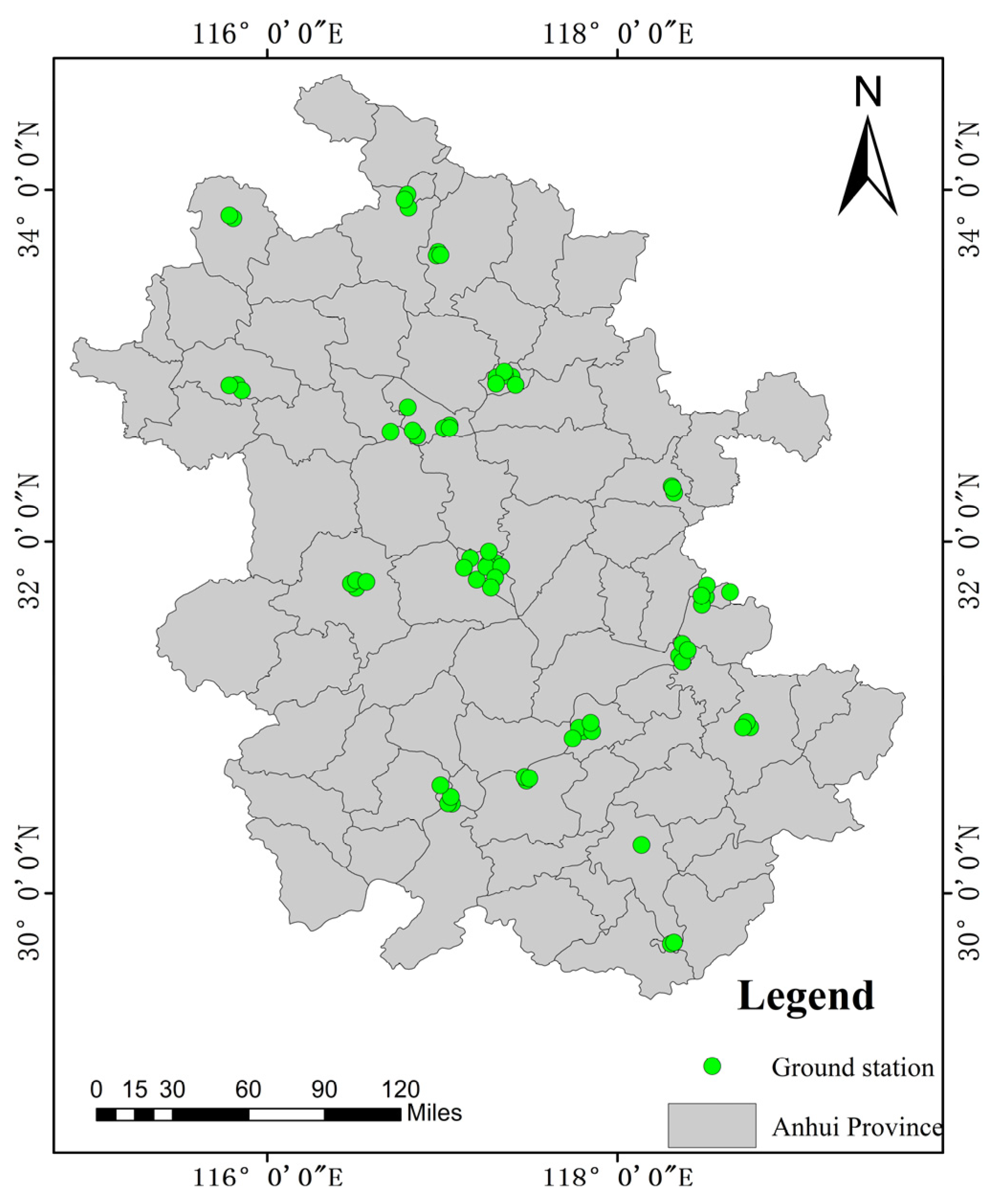
The research area in this paper was Anhui Province, located in the Yangtze River Delta region of China. The geographical location is between 114°54′ and 119°37′ east longitude and between 29°41′ and 34°38′ north latitude (Figure 1). The total area is 144,100 square kilometers. Anhui Province is in the transitional region between the warm temperate zone and the subtropical zone, with various terrains such as plains, hills, and mountains [34]. Due to the rapid economic development of the Yangtze River Delta, air pollution has always been a concern. According to the environmental quality report for the first half of 2020 issued by Anhui Province, the air pollutants in 16 prefecture-level cities showed significant regional characteristics. The proportions of days with mild, moderate, and severe pollution are 14.6%, 2.5%, and 1.0%, respectively. The days with PM2.5 as the primary pollutant are the most frequent. Therefore, it is of great significance to monitor PM2.5 using remote sensing methods.
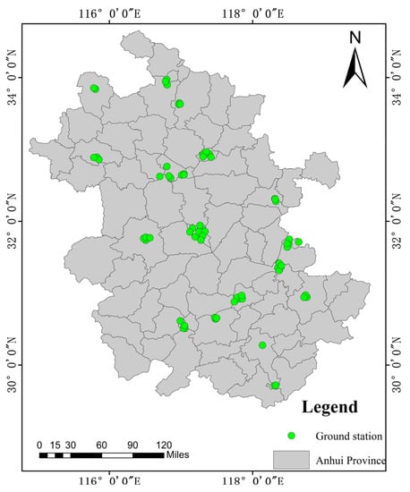
Figure 1.
Study area and PM2.5 ground station distribution.
2.2. MODIS Satellite Data
In this study, satellite data from the Moderate-Resolution Imaging Spectroradiometer (MODIS) mounted on Terra and Aqua satellites were used. The Terra satellite passes through the equator from north to south at about 10:30 a.m. local time. The Aqua satellite passes through the equator from south to north at about 1:30 p.m. local time. Their orbits are 705 km high, and the two satellites cooperate with each other to observe the entire earth’s surface repeatedly every 1–2 days, featuring a wide spectrum range. The data can be downloaded from NASA’s official website, including L1A products of MOD02_1 km and MYD02_1 km, which have 36 medium-resolution levels (0.4–14.4 μm) of spectral bands, covering the full spectrum from visible light to thermal infrared. The spatial resolution of two channels is 250 m, that of five channels is 500 m, and that of 29 channels is 1000 m. We applied the MODIS Conversion Toolkit (MCTK) for geometric correction, radiometric calibration, atmospheric correction, and other pre-processing operations to obtain MODIS satellite data for Anhui Province from 2016 to 2019. Then, the NDVI and NDBI, which were employed as the influencing factors of PM2.5 concentration, were calculated using the red, near-infrared, and shortwave infrared data in L1A products.
2.3. PM2.5 Measurements from Ground Stations
China’s National Ambient Air Quality Standard (GB3095–2012) stipulates that the PM2.5 concentrations at ground sites should be measured using the micro-oscillating balance method and the β-ray method [26]. As of 2020, China’s ground PM2.5 real-time monitoring network had more than 1700 stations. In this study, the hourly PM2.5 concentration data of effective sites in Anhui Province throughout the year from 2016 to 2019 were obtained through the China National Environmental Monitoring Center (CNEMC) website. The PM2.5 mass concentration unit was μg/m−3. The specific site distribution is shown in Figure 1.
2.4. Weather Reanalysis Data
In this study, the ERA5 hourly reanalysis dataset from the European Center for Medium-Range Weather Forecasts (ECMWF) was used. ERA5 is a reanalysis of global climate and weather data. It uses the laws of physics to combine model data with observations from all over the world into a global complete and consistent dataset. The spatial resolution of the ERA5 reanalysis dataset is 0.25° × 0.25°. Studies have shown that wind speed, temperature, humidity, rainfall, and other factors have a certain impact on PM2.5 concentration [35]. Referring to the existing research [27] and through experiments, this paper finally selected wind speed, boundary layer height, total amount of ozone column, boundary layer diffusion, temperature, evaporation, total precipitation, surface pressure, high-vegetation-cover index, low-vegetation-cover index, and relative humidity as auxiliary meteorological factors affecting PM2.5 concentration. The auxiliary meteorological factors are shown in Table 1.

Table 1.
Selected ERA5 reanalysis data.
ERA5 Accuracy Analysis
ECMWF was established in 1975 and is an international organization consisting of 34 countries. As one of the world’s meteorological centers, ECMWF has developed a global medium-term weather numerical forecast model that is at the forefront of the world. The ERA5 launched by ECMWF is currently the most powerful global climate atmospheric reanalysis tool, which provides hourly data and uncertainty estimates of various atmospheric, land and ocean state parameters. Additionally, it has also been widely used for atmospheric parameter estimation [36,37,38]. Existing studies [36,38,39,40] have shown the accuracy and applicability of wind speed and temperature in ERA5 data. Hersbach H et al. [41] as well showed the good performance of ERA5 data. Therefore, it can be seen from the above research that ERA5 has a good application prospect in atmospheric parameter estimation.
2.5. Data Preprocessing
Data pre-processing included MODIS remote sensing image pre-processing, data cleaning, removal of outliers, resampling, and data matching. We used the MCTK plug-in to pre-process MOD02/MYD02 km data in MODIS remote sensing image pre-processing, including radiometric calibration, geometric correction, atmospheric correction, Bowtie correction, reprojection, coordinate system conversion, and resampling. Then, we removed invalid data, such as null values, and resampled the meteorological reanalysis data to the same 1 km resolution as the MODIS remote sensing image. Finally, according to the latitude, longitude, and time, the MODIS data, the meteorological reanalysis data, and the PM2.5 mass concentration data of the ground station were matched spatiotemporally.
3. Methods
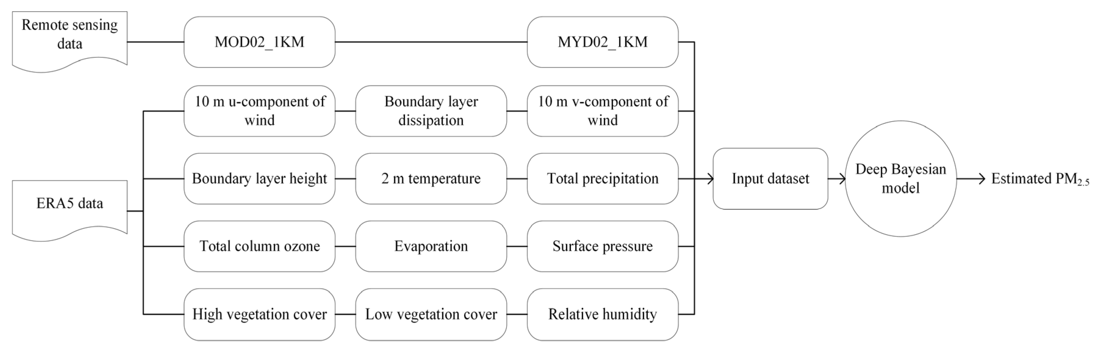
Figure 2 depicts the flow chart of PM2.5 modeling in Anhui Province used in this paper. The input of the model included MODIS, ERA5, and ground station data. In order to obtain data with the same projection and spatiotemporal resolution, the meteorological reanalysis data and MODIS data were pre-processed. After all the data were prepared, the deep Bayesian model was trained and verified, and the parameters were adjusted to obtain the optimal model; then, estimations and analyses were performed. We selected 5 × 5 km, 3 × 3 km, and 1 × 1 km neighborhoods in the surrounding space, before extracting their environmental characteristics. In order to verify the accuracy of the deep Bayesian model in this paper, the DNN [31] model, random forest model [28], and Bayesian neural network (BNN) model, without considering the surrounding impact, were used as comparison models.
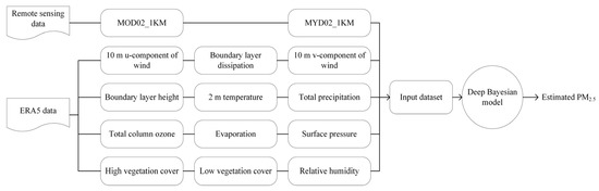
Figure 2.
Flow chart of the deep Bayesian model used to estimate PM2.5.
3.1. Impact Factor Screening
It is known from Robin Genuer, Carolin Strobl et al. [42,43] that the use of random forest is an effective method for variable selection in the variable selection problem of classification and regression. They used random forest to obtain the importance of the variables and sort them, and finally select the variables according to the importance of the variables. Therefore, in this study, the random forest model is used to select the best impact factor of ERA5 to reduce the redundancy of impact factors. The performance of the model is optimized by selecting the optimal permutation and combination of the influencing factors. On account of the decision tree generated using Boostrap, each tree in the random forest will not use all data samples in the production process. This part of the sample is called out-of-bag sample (oob). By using oob to iterate each feature, constantly changing the number of features, and comparing the oob scores before and after the model under the unchanged number of features, we are able to judge the importance of different features, sort the evaluation scores; the higher the score, the more important the feature, then, use the scores to combine from high to low, observe the changes in scores, and finally select the best feature combination.
3.2. Bayesian Neural Network
Neural networks have a strong nonlinear fitting ability; thus, they have a wide range of applications in various fields. For a neural network, the core task is to obtain the parameters of each layer of the network according to the data of the training set, and then optimize the parameters such that the loss function reaches a minimum. In reality, there is usually uncertainty within the data, and there is a certain randomness between x and y. However, a neural network lacks consideration of the model and uncertainty of the data; hence, when the amount of data is small, there is a serious overfitting phenomenon, leading to certain limitations in application. The Bayesian neural network is a type of neural network model. In a standard neural network, the weight parameter is represented by a single point, whereas the Bayesian neural network model parameter is not a fixed value; instead, the parameter is expressed in the form of a probability distribution to provide an uncertainty estimation. Furthermore, the parameters are expressed in the form of a prior probability distribution, and the average value is calculated for many models during training, such that the uncertainty of the model and data can be considered, and a regularization effect can be provided to the network. In addition, the Bayesian neural network has the advantage of being able to obtain a more robust model based on less training data, and it can obtain the distribution of parameters in each layer, thereby effectively preventing the problem of overfitting. The core of the Bayesian neural network is the Bayesian equation, presented below.
where (Y, X) are the training data; since the training data are given, P (Y, X) is a constant. The goal of the Bayesian neural network is to determine , where P (W) is the prior probability of W, and is the probability that the neural network outputs Y under the given parameters W and X.
However, the probability distribution of is complicated and difficult to solve. Therefore, the Bayesian neural network approximates the P function by establishing a q function, and then uses a simpler distribution to approximate . The average μ and standard deviation σ parameters of the P function are the parameters that need to be adjusted by the neural network. Bayesian neural networks generally select two distributions of KL divergence to judge the effect of the q function approaching the P function. KL divergence is also called the relative entropy of two distributions, which is used to measure the distance between two random variables. KL divergence is a measure of the difference between two probability distributions p and q, and its mathematical definition is as follows:
Further analysis obtains
It can be obtained that the KL divergence is the expectation about q. The Adam optimizer can be used to obtain the optimal parameters, minimize the KL divergence, and obtain the optimal model.
3.3. Deep Bayesian Model
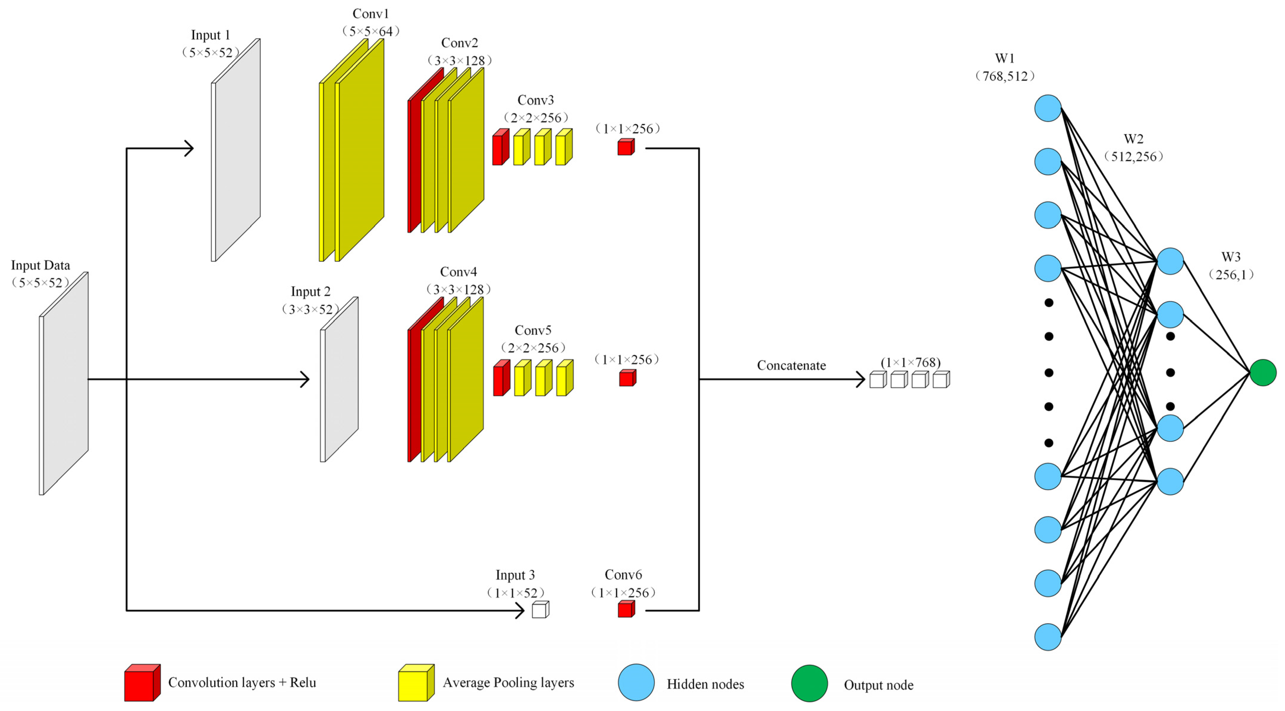
The deep Bayesian model is composed of an input layer, a hidden layer, and an output layer. This model used MODIS satellite data as the main input, along with meteorological reanalysis data, NDVI, and NDBI as auxiliary data. The PM2.5 modeling equation was as follows:
where the dependent variable is PM2.5 concentration, α1, …, α38 represent data from the 38 bands of the MODIS satellite, and β1, …, β14 represent the 14 auxiliary data.
In addition, in order to better consider the impact of the surrounding environment on the PM2.5 concentration, the environmental characteristics of the surrounding 5 × 5 km, 3 × 3 km, and 1 × 1 km spaces were extracted. The deep Bayesian model designed in this paper is shown in Figure 3. In the input layer of the model, the input data were 5 × 5 × 52. Because the band data of the MODIS satellite and the dimensions of the meteorological reanalysis data were not uniform, this paper designed a standardization module to standardize all the data and unify their dimensions to the same order of magnitude. Moreover, standardization allows avoiding the adverse effects of outliers and extreme values via centralization. The standardized sample data conform to a standard normal distribution, i.e., with a mean of 0 and a standard deviation of 1. The standardization equation is as follows:
where is the standardized data, is the original data, is the average of all sample data, and is the standard deviation of all sample data.
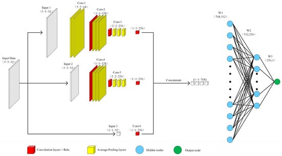
Figure 3.
Structure diagram of deep Bayesian model.
In order to fully consider the influence of the surrounding neighborhood on the PM2.5 concentration, this model performs feature extraction at three different scales of 5 × 5 km, 3 × 3 km, and 1 × 1 km, and then performs feature fusion. As the model is trained and the depth of the model is deepened, the distribution of the input of the hidden layer changes or shifts, which causes the model to converge slowly. Therefore, the model in this paper introduced the batch normalization (BN) method after each hidden layer to accelerate the process of model training convergence. BN uses a certain standardization method to forcibly transform the input distribution of each hidden layer back to a standard normal distribution with a mean of 0 and a standard deviation of 1. As the depth of the model increases, the number of parameters increases, which causes the problem of model overfitting. Therefore, the model in this paper introduced a dropout layer after each hidden layer to reduce the complex connection between neurons, increase the orthogonality between the features of each layer, and make the learned network model more robust. In the optimization process, it is also possible to prevent the parameters from oscillating at the local optimum and improve the performance of the model. Moreover, using the Bayesian neural network, the uncertainty of the model and data can be considered; therefore, a more robust model can be obtained on the basis of less data, and the distribution of the parameters of each layer can be obtained. This allows overcoming the problem of model overfitting better, thereby not only predicting the result but also effectively predicting its error. The activation function of each hidden layer used in the model was a linear ReLU function, and the output layer produced the estimated value of PM2.5 mass concentration.
As the core guide for model optimization learning, the loss function needs to be minimized during model training. This paper selected the mean square error (MSE), one of the most commonly used loss functions in regression tasks, which can be expressed as follows:
where n is the number of samples, is the estimated value of the model, and is the observation value of the ground station.
The learning rate is a crucial hyperparameter in deep learning, which determines the time for the objective function to converge to a minimum and whether it can converge to a local minimum. Thus, appropriate setting of this rate enables convergence of the objective function in an appropriate time. With respect to the deep Bayesian model in this article, learning rate was also used to scale the model weight update range to minimize the parameters of the model output deviation. Under normal circumstances, if the learning rate is too small, the process of model convergence becomes very slow, whereas, when it is too large, the gradient may oscillate around the minimum value and may even inhibit convergence [27]. After the model parameters were adjusted and tested many times, the initial learning rate of the deep Bayesian model was set to 0.001. Furthermore, the learning rate was reduced when the performance of the model was not improved following each iteration (15 rounds) during the training process. The total number of iterations of the model was set to 150.
3.4. Model Evaluation
Considering the spatial distribution of ground monitoring sites in Anhui Province, this paper extracted data from 68 of the 78 ground monitoring sites as a dataset for model training. The remaining 10 sites did not participate in training; instead, they were used as an independent testing dataset to evaluate the accuracy of the model. The training dataset was randomly divided into 80% for model training and 20% for verification. In this paper, the coefficient of determination (R2) and root mean square error (RMSE) were used to quantitatively evaluate the performance of the model.
R2 is the ratio of the regression sum of squares to the total deviation of squares. In model evaluation, a larger ratio denotes a higher accuracy and a more significant effect of the corresponding model. Generally speaking, the value of R2 lies between 0–1. A closer value to 1 denotes a better model fit, while a closer value to 0 indicates worse model fit. RMSE is defined as the square root of the ratio of the model’s estimated value to the observed value of the site, which is used to describe the degree of dispersion between both values. The equations for calculating R2 and RMSE are as follows:
where is the observed value of the site, is the mean value, and is the estimated value of the model.
4. Result
4.1. Results of Impact Factor Screening
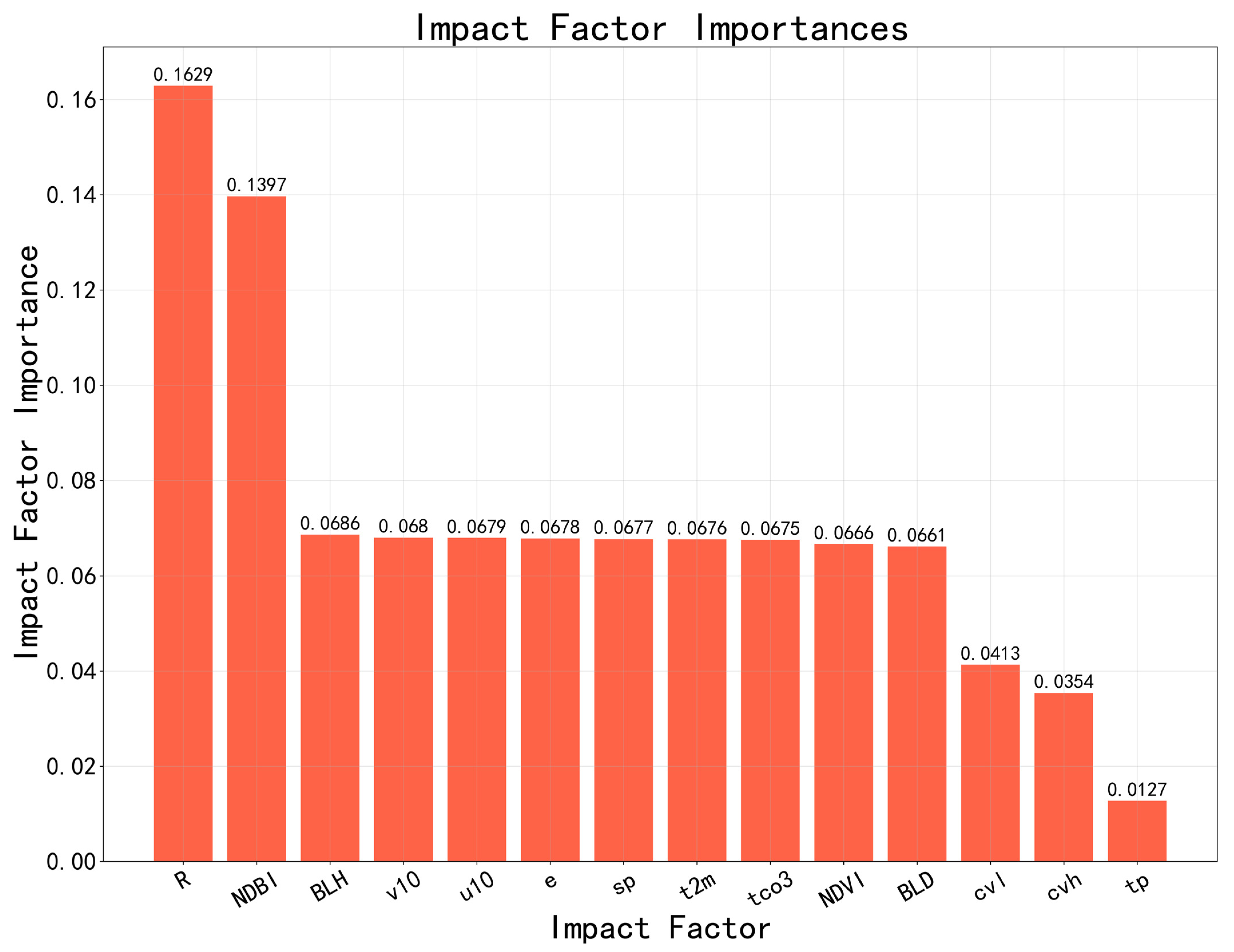
Figure 4 shows the importance ranking results of the Relative humidity (R), Normalized Difference Building Index(NDBI), Boundary Layer Height(BLH), 10 m v-component of wind(v10), 2 m temperature(t2m), Evaporation(e), Surface pressure(sp), 10 m u-component of wind(u10), total column ozone(tco3), Normalized Difference Vegetation Index (NDVI), Boundary layer dissipation(bld), low vegetation cover(cvl), high vegetation cover(cvh), total precipitation(tp) reanalysis data used in this model using random forest. It can be seen from the figure that these parameters play a positive role in the model’s estimation of PM2.5 concentration. Among them, tco3 and sp also showed high importance. In addition, Min Shao et al. [44] also analyzed the relationship between O3 and PM2.5 concentration from the perspective of chemical reactions and demonstrated the interaction between O3 and PM2.5. The influence of tco3 on PM2.5 concentration mainly comes from the influence of near-ground O3 on PM2.5 concentration. A variety of influencing factors (such as ground pressure, wind components, boundary layer characteristics, and precipitation) are used as input to the model. It mainly considers the comprehensive influence of various influencing factors on PM2.5 concentration. In summary, R, NDBI, blh, v10, t2m, e, sp, u10, tco3, NDVI, bld, cvl, cvh, tp as influencing factors play a positive role in the estimation accuracy of the model. So, we chose these factors as the influence factors of PM2.5 concentration.
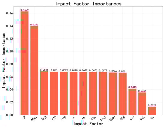
Figure 4.
Impact factor screening results.
4.2. Comparative Analysis of Model Results
4.2.1. Comparative Analysis of Different Methods
We performed model training on the prepared sample data. Figure 5 shows the training results of the deep Bayesian model in this article, as well as the results of the DNN, random forest, and Bayesian neural network models without consideration of the influence of the surrounding environment. It can be seen from Figure 5 that the deep Bayesian model showed high accuracy with the training data, with an R2 of 0.97. The DNN, random forest, and Bayesian neural network models also showed good accuracy with the training data, with R2 values of 0.92, 0.93, and 0.94, respectively. Among the four models, the deep Bayesian model had the lowest RMSE with the training data, at only 6.84 μg·m−3. It can be seen that the deep Bayesian model had the highest training accuracy, whereas the DNN model that did not consider the influence of the surrounding environment on the PM2.5 concentration had the lowest training accuracy.
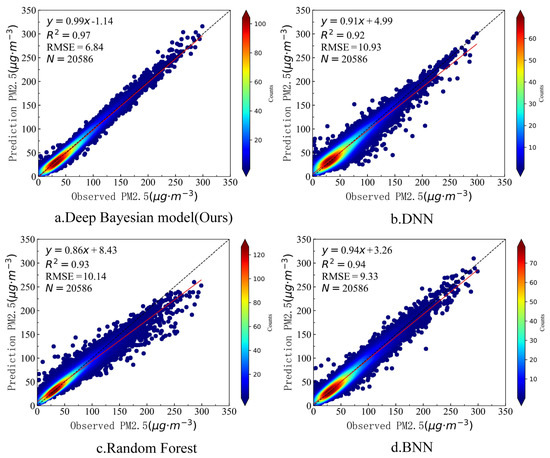
Figure 5.
Training accuracy of the four models.
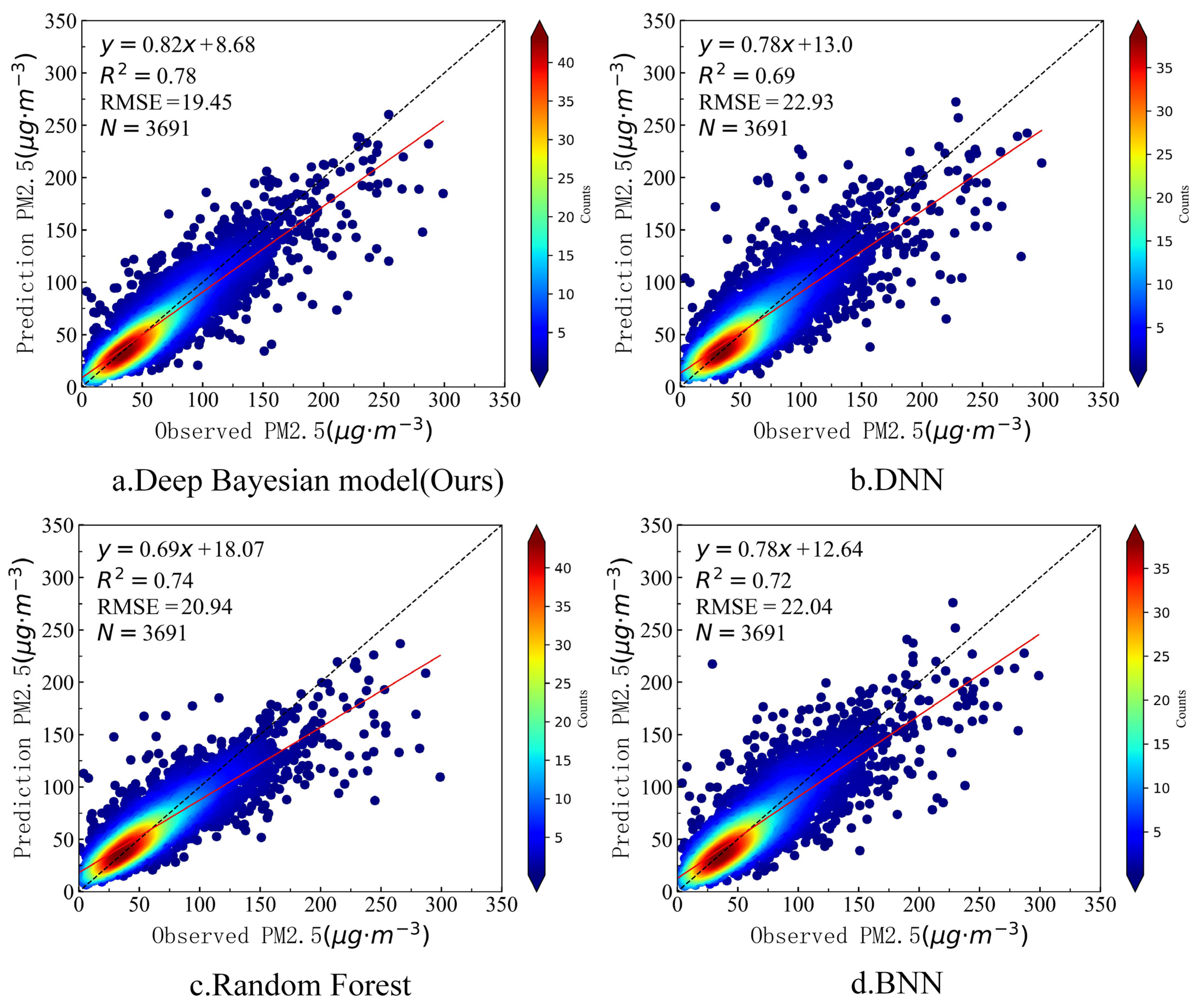
In order to better verify the estimation accuracy of the model in the study area, we used the deep Bayesian model in this paper, as well as the DNN, random forest, and BNN models without consideration of the impact of the surrounding environment, to estimate the PM2.5 concentration in the study area using the data from the 10 sites not participating in training. Figure 6 shows the accuracies of the four models with the test data. It can be seen from Figure 6 that the deep Bayesian model in this paper had the highest R2 with the test data, reaching 0.78, which was 9%, 4%, and 6% higher than the other three models. The deep Bayesian model in this paper also had the lowest RMSE, at only 19.45 μg·m−3, which was lower than the other three models by 3.48 μg·m−3, 1.49 μg·m−3, and 2.59 μg·m−3, respectively. It can be seen from Table 2 that the accuracy of the deep Bayesian model in this paper was better than that of the other three models for both the training set and the test set.

Figure 6.
Test accuracy of the four models.
Table 2.
Training and testing accuracy of the four models.
4.2.2. Spatial Scope Impact Analysis
In order to verify the influence of the size of the surrounding space domain, the accuracies of the models considering different ranges of 5 km × 5 km, 3 km × 3 km, and 1 km × 1 km were compared and analyzed. The results are presented below.
It can be seen from Table 3 that the models considering the different space domains had different accuracies. The highest accuracy was achieved when all three space domains were considered simultaneously. Therefore, this paper chose to extract features from the surrounding 1 km × 1 km, 3 km × 3 km, and 5 km × 5 km spatial domains as the influencing factors of PM2.5 concentration to construct a deep Bayesian model.
Table 3.
Comparison of the impact of different spatial ranges on model accuracy.
4.3. PM2.5 Concentration Estimation and Evaluation
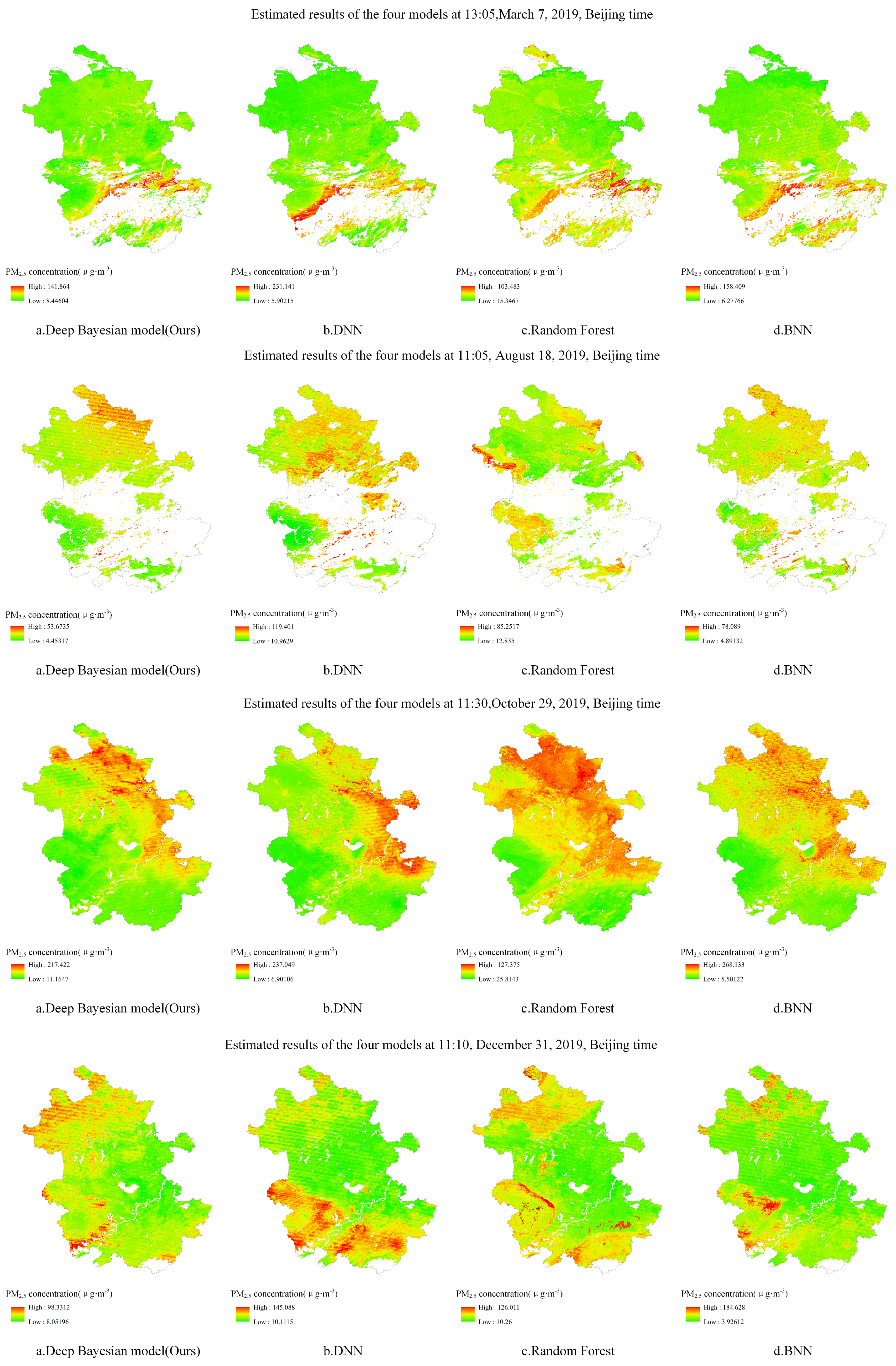
The deep Bayesian model of this paper, as well as the DNN, random forest, and BNN without consideration of the impact of the surrounding environment, was used to estimate the PM2.5 concentration of Anhui Province with the same spatial resolution (1 km) for comparative analysis. Figure 7 shows the false-color images of the regional MODIS satellites in Anhui Province at 1:05 p.m. on 7 March, 11:05 a.m. on 18 August, 11:30 a.m. on 29 October, and 11:10 a.m. on 31 December, Beijing time. Figure 8 shows the PM2.5 distribution at the four times estimated by the deep Bayesian, DNN, random forest, and BNN models. The blank areas in the figure denote where the surface water and clouds were removed from the satellite images. In the estimated PM2.5 distribution map, dark red denotes a high PM2.5 concentration, whereas dark green denotes a lower PM2.5 concentration. It can be seen from the figure that the results of PM2.5 estimation using the deep Bayesian model, as well as the DNN, random forest, and BNN models, were roughly the same in terms of spatial distribution; however, there were subtle differences in the estimation results of the different models. On 7 March 2019, the concentration in the central and eastern parts of Anhui Province showed a higher trend. The PM2.5 concentration estimated using the deep Bayesian model in the southwestern region was lower than the estimated concentration of the other three models. On 18 August 2019, there was a trend of lower concentrations in regions except for north-eastern Anhui Province. The PM2.5 concentration estimated by the random forest model was higher than that estimated by the other three models in the central and western regions. On 29 October 2019, there was a trend of higher concentrations in north-eastern and central-eastern Anhui Province, along with lower concentrations in other regions. The PM2.5 concentration estimated using the DNN model was lower than that estimated by the other three models in north-eastern Anhui Province. Moreover, the PM2.5 concentration estimated using the random forest model was higher in north-eastern Anhui Province than that estimated by the other three models. On 31 December 2019, the concentration in central and eastern Anhui Province was lower than the remainder of the region. The estimation results of the deep Bayesian model and the random forest model in central-western Anhui Province were higher than those of the DNN and BNN models.
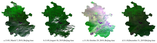
Figure 7.
False-color map of regional MODIS satellites in Anhui Province at four timepoints.
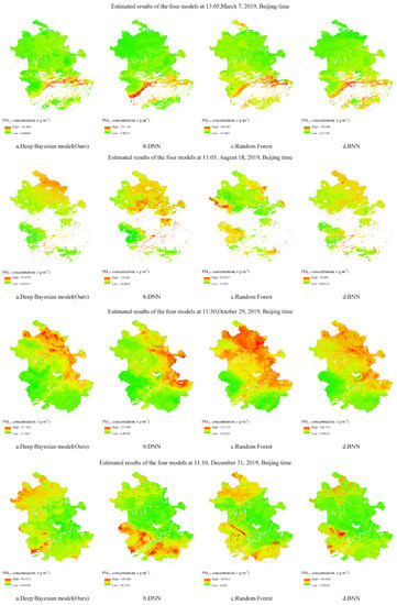
Figure 8.
Model estimation results of Anhui Province at four timepoints.
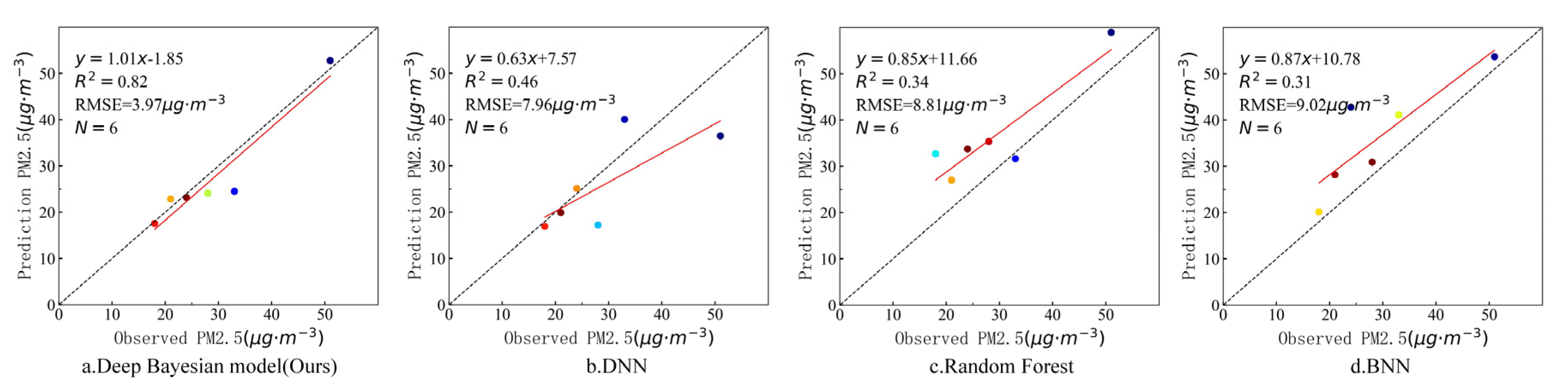
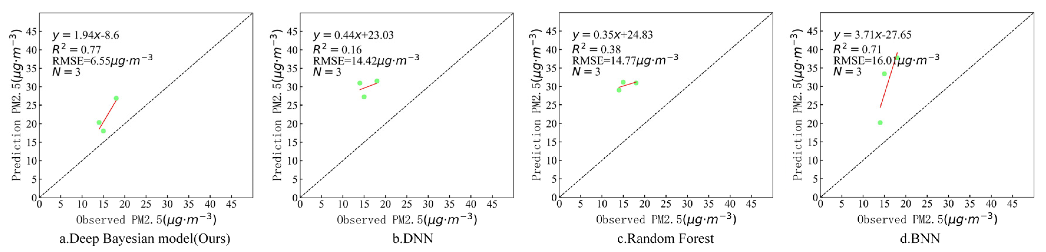
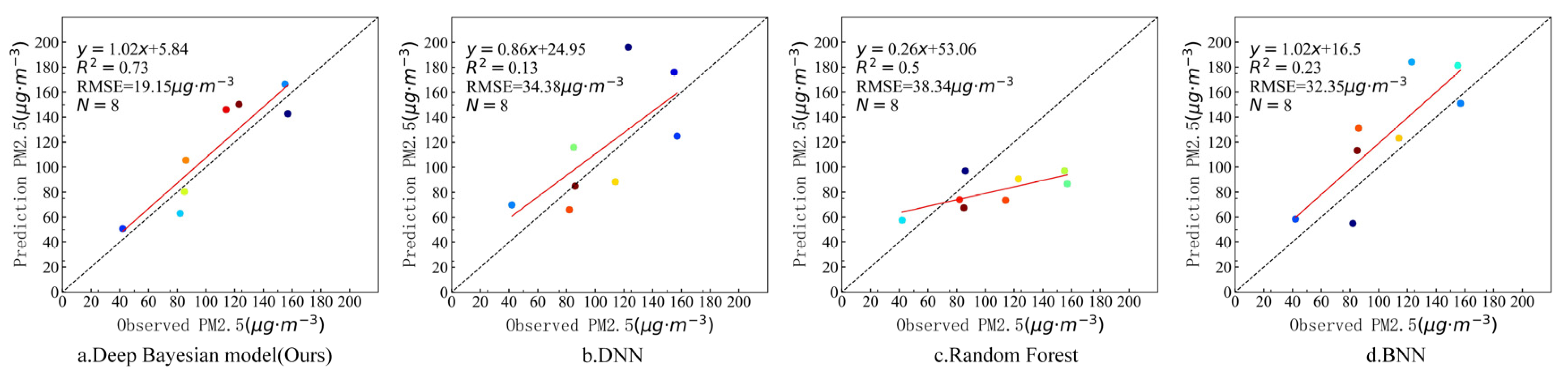
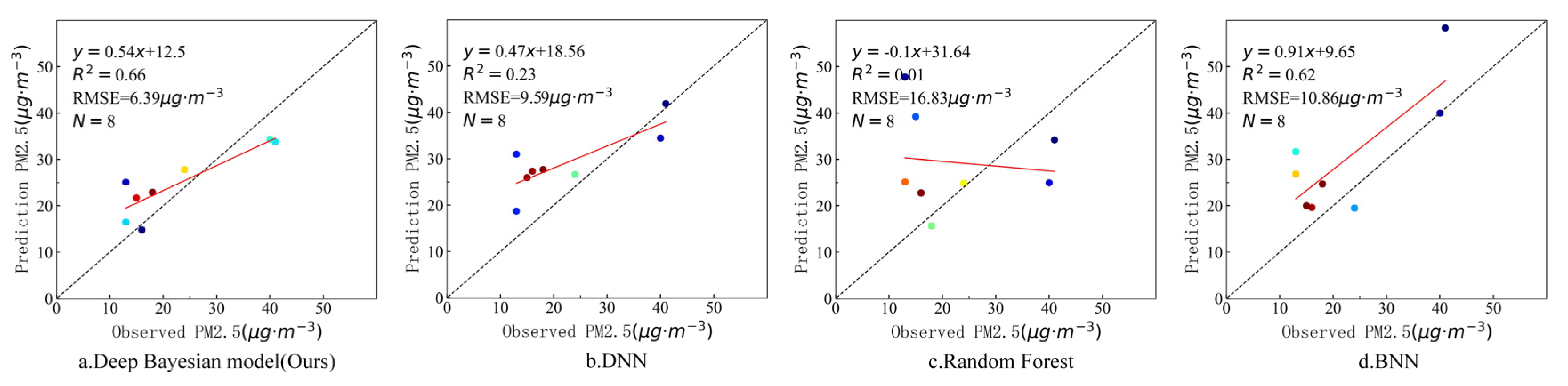
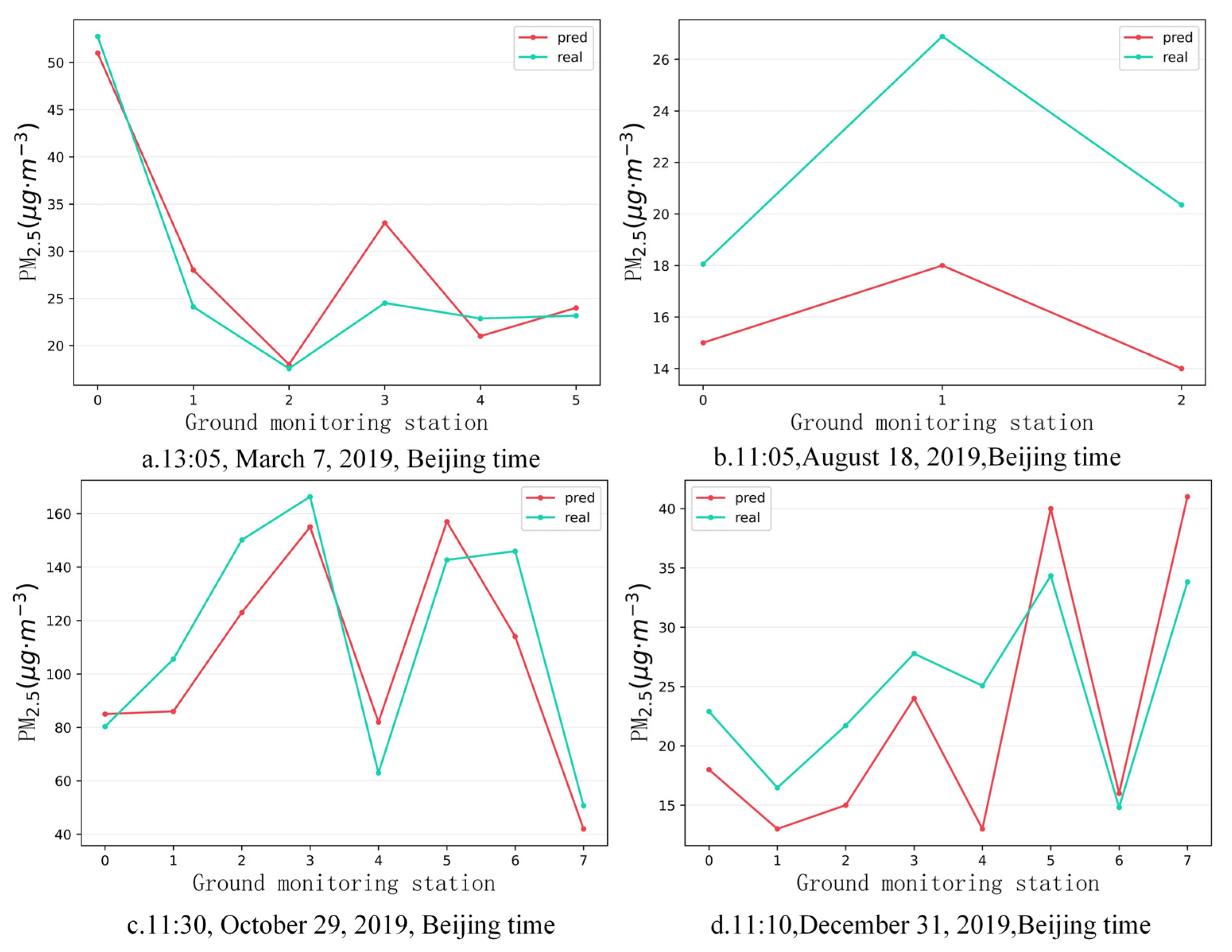
In order to further verify the estimation accuracy of the model, the observed values of the independent test sites that did not participate in training at the above four timepoints were compared with the estimated values of the model. There were six valid sites that were not blocked by clouds on 7 March, three valid sites that were not blocked by clouds on 18 August, and eight valid sites that were not blocked by clouds on 29 October and 31 December. Figure 9, Figure 10, Figure 11 and Figure 12 show the estimation accuracy statistics of the four models for the valid sites at the four timepoints. The estimation results in terms of R2 of the deep Bayesian model at the four timepoints were 0.82, 0.77, 0.73, and 0.66, all of which were higher than the values obtained for the DNN, random forest, and BNN models. The RMSE values were 3.97, 6.55, 19.15, and 6.39 µg·m−3, all of which were lower than the values obtained for the DNN, random forest, and BNN models. It can be seen that the accuracy of the deep Bayesian model in this paper was better than that of the other three models, and its generalization ability was also better. Figure 13 demonstrates that the values estimated by the deep Bayesian model for the valid sites at the four timepoints were in good agreement with the values observed at the ground site.
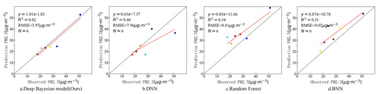
Figure 9.
Scatter plot of the estimated values by the four models and the observed values at the sites at 1:05 p.m., 7 March 2019.
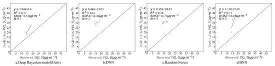
Figure 10.
Scatter plot of the estimated values by the four models and the observed values at the sites at 11:05 a.m., 18 August 2019.
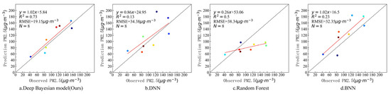
Figure 11.
Scatter plot of the estimated values by the four models and the observed values at the sites at 11:30 a.m., 29 October 2019.
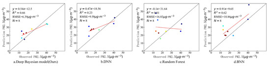
Figure 12.
Scatter plot of the estimated values by the four models and the observed values at the sites at 11:10 a.m., 31 December 2019.
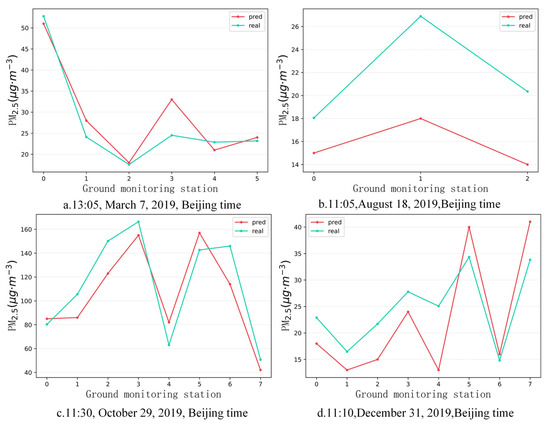
Figure 13.
Trends of the estimated and observed values at the four timepoints.
5. Discussion
The independent test set of non-training data can be seen from the comparison results of different methods (Figure 6). Compared with the single-pixel-based DNN model, random forest model and Bayesian neural network model, the estimation accuracy of the method proposed in this paper that takes into account spatial multi-scale has been improved by 9%, 4%, and 6%, respectively. The main reason for this improvement is that the method in this paper not only combines the characteristics of the Bayesian neural network to consider uncertainty, but also regards the atmosphere as a complex whole, and uses multi-scale features as the input of the model. This can provide the model with uncertainty considerations and perception of features at different scales and strengthen the model’s ability to extract and integrate features at different scales, thereby improving the accuracy of the model. Considering the depth Bayesian model of this article to estimate PM2.5 concentration at four different time points in 2019, from the estimation results (Figure 9, Figure 10, Figure 11 and Figure 12), it can be seen that on the effective non-training site, when the accuracy of other comparison models decreases, the model in this paper still has good accuracy and the accuracy is higher than that of the comparison model. This fully demonstrates that the model in this paper combines the characteristics of the Bayesian neural network with the consideration of uncertainty, which allows the model in this paper retain better model generalization capabilities.
In general, the comparative analysis with different methods has fully verified that the deep Bayesian model proposed in this paper can effectively improve the model estimation accuracy and the generalization ability of the model under the condition of taking into account multi-scale features. However, due to the limitation of the time resolution of MODIS satellites, its Terra satellites and Aqua satellites only transit at around 10:30 am local time and 1:30 pm local time, respectively. Therefore, the method in this paper still has the problem that it cannot provide PM2.5 monitoring results with higher time resolution. We will use high time resolution satellite data in future research to improve the time resolution of PM2.5 monitoring results.
6. Conclusions
This paper designed a deep Bayesian PM2.5 estimation model taking into account multiple scales. The model uses a Bayesian neural network to describe key parameters a priori, provide regularization effects to the neural network, perform posterior inference through parameters, and take into account the characteristics of data uncertainty. It can be used to alleviate the problem of model overfitting and to improve the generalization ability of the model. We used different-scale MODIS satellite MOD02_1 km/MYD02_1 km, NDVI, NDBI, and ERA5 reanalysis data as the input of the model, strengthened the model’s perception of different-scale features of the surrounding atmosphere, and further improved the model’s PM2.5 concentration estimation accuracy and model generalization ability. Experiments in Anhui Province as the research area showed that the R2 and RMSE of this method on the independent test set were 0.78 and 19.45 μg·m−3, respectively. Compared with the three models of DNN, random forest, and Bayesian neural network that did not consider the surrounding environment, the R2 was increased by 9%, 4%, and 6%, and the RMSE was reduced by 3.48 μg·m−3, 1.49 μg·m−3, and 2.59 μg·m−3, respectively. In the experiment of different seasons in 2019, compared with the other three models, the estimation accuracy of PM2.5 was significantly reduced; however, the R2 of the model in this paper could still reach 0.66 or more. In addition, the estimation results were in good agreement with the trend of observations at ground stations. Through experimental comparison and analysis, it can be found that the single-pixel information estimation method, considering the influence of the surrounding environment on the PM2.5 concentration, can greatly improve the accuracy of the model. This shows that the surrounding environment has a great influence on the PM2.5 concentration; thus, taking the surrounding environment as an influencing factor of the PM2.5 concentration can improve the estimation accuracy of the model. Combined with the characteristics of the BNN, considering the uncertainty of the data can improve the generalization ability of the model, reduce the problem of model overfitting, and further improve the estimation accuracy of the model.
Author Contributions
Conceptualization, X.C. and Y.W.; methodology, X.C. and Y.W.; software, Y.W.; validation, P.J.; resources, Y.W.; data curation, P.K.; writing—original draft preparation, X.C.; writing—review and editing, Y.W., P.J. and P.K.; funding acquisition, Y.W. All authors have read and agreed to the published version of the manuscript.
Funding
This study was primarily supported by the National Natural Science Foundation of China (grant No. 41971311), and Technology Major Project of Anhui Province(grant No.18030801111).
Institutional Review Board Statement
Not applicable.
Informed Consent Statement
Not applicable.
Data Availability Statement
Publicly available datasets were analyzed in this study.
Conflicts of Interest
The authors declare no conflict of interest.
References
- Luo, H.; Guan, Q.; Lin, J.; Wang, Q.; Yang, L.; Tan, Z.; Wang, N. Air pollution characteristics and human health risks in key cities of northwest China. J. Environ. Manag. 2020, 269, 110791. [Google Scholar] [CrossRef] [PubMed]
- Yang, G.; Wang, Y.; Zeng, Y.; Gao, G.F.; Liang, X.; Zhou, M.; Wan, X.; Yu, S.; Jiang, Y.; Naghavi, M.; et al. Rapid health transition in China, 1990–2010: Findings from the Global Burden of Disease Study 2010. Lancet 2013, 381, 1987–2015. [Google Scholar] [CrossRef]
- Wang, J.; Cristopher, S.A. Intercomparison between satellite-derived aerosol optical thickness and PM2.5 mass: Implications for air quality studies. Geophys. Res. Lett. 2003, 30, 2095. [Google Scholar] [CrossRef]
- Li, R.; Mei, X.; Chen, L.; Wang, Z.; Jing, Y.; Wei, L. Influence of spatial resolution and retrieval frequency on applicability of satellite-predicted PM2.5 in Northern China. Remote Sens. 2020, 12, 736. [Google Scholar] [CrossRef] [Green Version]
- van Donkelaar, A.; Martin, R.V.; Brauer, M.; Hsu, C.; Kahn, R.A.; Levy, R.C.; Lyapustin, A.; Sayer, A.M.; Winker, D.M. Global estimates of fine particulate matter using a combined geophysical-statistical method with information from satellites, models, and monitors. Environ. Sci. Technol. 2016, 50, 3762–3772. [Google Scholar] [CrossRef] [PubMed]
- He, Q.; Huang, B. Satellite-based mapping of daily high-resolution ground PM2.5 in China via space-time regression modeling. Remote Sens. Environ. 2018, 206, 72–83. [Google Scholar] [CrossRef]
- Koelemeijer, R.B.A.; Homan, C.D.; Matthijsen, J. Comparison of spatial and temporal variations of aerosol optical thickness and particulate matter over Europe. Atmos. Environ. 2006, 40, 5304–5315. [Google Scholar] [CrossRef]
- Lin, C.; Li, Y.; Lau, A.; Deng, X.; Tse, T.K.; Fung, J.; Li, C.; Li, Z.; Lu, X.; Zhang, X.; et al. Estimation of long-term population exposure to PM2.5 for dense urban areas using 1-km MODIS data. Remote Sens. Environ. 2016, 179, 13–22. [Google Scholar] [CrossRef] [Green Version]
- Zhang, Y.; Li, Z. Remote sensing of atmospheric fine particulate matter (PM2.5) mass concentration near the ground from satellite observation. Remote Sens. Environ. 2015, 160, 252–262. [Google Scholar] [CrossRef]
- Gupta, P.; Christopher, S.A. Seven year particulate matter air quality assessment from surface and satellite measurements. Atmos. Chem. Phys. 2008, 8, 3311–3324. [Google Scholar] [CrossRef] [Green Version]
- Meng, X.; Fu, Q.; Ma, Z.; Chen, L.; Zou, B.; Zhang, Y.; Xue, W.; Wang, J.; Wang, D.; Kan, H.; et al. Estimating ground-level PM (10) in a Chinese city by combining satellite data, meteorological information and a land use regression model. Environ. Pollut. 2016, 208, 177–184. [Google Scholar] [CrossRef] [PubMed]
- Lee, H.J.; Liu, Y.; Coull, B.A.; Schwartz, J.; Koutrakis, P. A novel calibration approach of MODIS AOD data to predict PM 2.5 concentrations. Atmos. Chem. Phys. 2011, 11, 7991–8002. [Google Scholar] [CrossRef] [Green Version]
- Liu, Y.; Sarnat, J.A.; Kilaru, V.; Jacob, D.J.; Koutrakis, P. Estimating ground-level PM2.5 in the Eastern United States using satellite remote sensing. Environ. Sci. Technol. 2005, 39, 3269–3278. [Google Scholar] [CrossRef] [Green Version]
- van Donkelaar, A.; Martin, R.V.; Spurr, R.J.D.; Burnett, R.T. High-resolution satellite-derived PM2.5 from optimal estimation and geographically weighted regression over North America. Environ. Sci. Technol. 2015, 49, 10482–10491. [Google Scholar] [CrossRef] [PubMed]
- Yang, Q.; Yuan, Q.; Yue, L.; Li, T.; Shen, H.; Zhang, L. The relationships between PM2.5 and aerosol optical depth (AOD) in mainland China: About and behind the spatio-temporal variations. Environ. Pollut. 2019, 248, 526–535. [Google Scholar] [CrossRef] [PubMed]
- You, W.; Zang, Z.; Zhang, L.; Zhang, M.; Pan, X.; Li, Y. A nonlinear model for estimating ground-level PM10 concentration in Xi’an using MODIS aerosol optical depth retrieval. Atmos. Res. 2016, 168, 169–179. [Google Scholar] [CrossRef]
- He, J.; Christakos, G. Space-time PM2.5 mapping in the severe haze region of Jing-Jin-Ji (China) using a synthetic approach. Environ. Pollut. 2018, 240, 319–329. [Google Scholar] [CrossRef] [PubMed]
- Brokamp, C.; Jandarov, R.; Hossain, M.; Ryan, P. Predicting daily urban fine particulate matter concentrations using a random forest model. Environ. Sci. Technol. 2018, 52, 4173–4179. [Google Scholar] [CrossRef] [PubMed]
- Xu, Y.; Ho, H.C.; Wong, M.S.; Deng, C.; Shi, Y.; Chan, T.-C.; Knudby, A. Evaluation of machine learning techniques with multiple remote sensing datasets in estimating monthly concentrations of ground-level PM2.5. Environ. Pollut. 2018, 242, 1417–1426. [Google Scholar] [CrossRef] [PubMed]
- Li, T.; Shen, H.; Yuan, Q.; Zhang, L. Geographically and temporally weighted neural networks for satellite-based mapping of ground-level PM2.5. ISPRS J. Photogramm. Remote Sens. 2020, 167, 178–188. [Google Scholar] [CrossRef]
- Li, T.; Shen, H.; Zeng, C.; Yuan, Q.; Zhang, L. Point-surface fusion of station measurements and satellite observations for mapping PM2.5 distribution in China: Methods and assessment. Atmos. Environ. 2017, 152, 477–489. [Google Scholar] [CrossRef] [Green Version]
- Murillo-Escobar, J.; Sepulveda-Suescun, J.P.; Correa, M.A.; Orrego-Metaute, D. Forecasting concentrations of air pollutants using support vector regression improved with particle swarm optimization: Case study in Aburrá Valley, Colombia. Urban Clim. 2019, 29, 100473. [Google Scholar] [CrossRef]
- Qiao, J.; He, Z.; Du, S. Prediction of PM2.5 concentration based on weighted bagging and image contrast-sensitive features. Stoch. Environ. Res. Risk Assess. 2020, 34, 561–573. [Google Scholar] [CrossRef]
- Tao, M.; Wang, Z.; Tao, J.; Chen, L.; Wang, J.; Hou, C.; Wang, L.; Xu, X.; Zhu, H. How do aerosol properties affect the temporal variation of MODIS AOD bias in Eastern China? Remote Sens. 2017, 9, 800. [Google Scholar] [CrossRef] [Green Version]
- Song, Z.; Fu, D.; Zhang, X.; Han, X.; Song, J.; Zhang, J.; Wang, J.; Xia, X. MODIS AOD sampling rate and its effect on PM2.5 estimation in North China. Atmos. Environ. 2019, 209, 14–22. [Google Scholar] [CrossRef]
- Tao, M.; Wang, J.; Li, R.; Wang, L.; Wang, L.; Tao, J.; Che, H.; Chen, L. Performance of MODIS high-resolution MAIAC aerosol algorithm in China: Characterization and limitation. Atmos. Environ. 2019, 213, 159–169. [Google Scholar] [CrossRef]
- Mao, F.; Hong, J.; Min, Q.; Gong, W.; Zang, L.; Yin, J. Estimating hourly full-coverage PM2.5 over China based on TOA reflectance data from the Fengyun-4 A satellite. Environ. Pollut. 2021, 270, 116119. [Google Scholar] [CrossRef] [PubMed]
- Liu, J.; Weng, F.; Li, Z. Satellite-based PM2.5 estimation directly from reflectance at the top of the atmosphere using a machine learning algorithm. Atmos. Environ. 2019, 208, 113–122. [Google Scholar] [CrossRef]
- Shen, H.; Li, T.; Yuan, Q.; Zhang, L. Estimating regional ground-level PM2.5 Directly from satellite top-of-atmosphere reflectance using deep belief networks. J. Geophys. Res. Atmos. 2018, 123, 13–875. [Google Scholar] [CrossRef] [Green Version]
- Bai, H.; Zheng, Z.; Zhang, Y.; Huang, H.; Wang, L. Comparison of satellite-based PM2.5 Estimation from aerosol optical depth and top-of-atmosphere reflectance. Aerosol Air Qual. Res. 2020, 21, 200257. [Google Scholar] [CrossRef]
- Imani, M. Particulate matter (PM2.5 and PM10) generation map using MODIS Level-1 satellite images and deep neural network. J. Environ. Manag. 2021, 281, 111888. [Google Scholar] [CrossRef] [PubMed]
- Hong, K.Y.; Pinheiro, P.O.; Weichenthal, S. Predicting global variations in outdoor PM2.5 concentrations using satellite images and deep convolutional neural networks. arXiv 2019, arXiv:1906.03975. [Google Scholar]
- Zheng, T.; Bergin, M.H.; Hu, S.; Miller, J.; Carlson, D.E. Estimating ground-level PM 2.5 using micro-satellite images by a convolutional neural network and random forest approach. Atmos. Environ. 2020, 230, 117451. [Google Scholar] [CrossRef]
- Li, G.; Wu, H.; Zhong, Q.; He, J.; Yang, W.; Zhu, J.; Zhao, H.; Zhang, H.; Zhu, Z.; Huang, F. Six air pollutants and cause-specific mortality: A multi-area study in nine counties or districts of Anhui Province, China. Environ. Sci. Pollut. Res. 2021, 1–15. [Google Scholar] [CrossRef] [PubMed]
- Wu, P.; Sun, J.; Chang, X.; Zhang, W.; Arcucci, R.; Guo, Y.; Pain, C.C. Data-driven reduced order model with temporal convolutional neural network. Comput. Methods Appl. Mech. Eng. 2020, 360, 112766. [Google Scholar] [CrossRef]
- Liu, B.; Guo, J.; Gong, W.; Zhang, Y.; Shi, L.; Ma, Y.; Li, J.; Guo, X.; Stoffelen, A.; de Leeuw, G.; et al. Intercomparison of wind observations from ESA’s satellite mission Aeolus, ERA5 reanalysis and radiosonde over China. Atmos. Chem. Phys. 2021, 1–35. [Google Scholar] [CrossRef]
- Shikhovtsev, A.Y.; Bolbasova, L.A.; Kovadlo, P.G.; Kiselev, A.V. Atmospheric parameters at the 6-m Big Telescope Alt-azimuthal site. Mon. Not. R. Astron. Soc. 2020, 493, 723–729. [Google Scholar] [CrossRef]
- Demchev, D.M.; Kulakov, M.Y.; Makshtas, A.P.; Makhotina, I.A.; Fil’chuk, K.V.; Frolov, I.E. Verification of ERA-Interim and ERA5 Reanalyses Data on Surface Air Temperature in the Arctic. Russ. Meteorol. Hydrol. 2020, 45, 771–777. [Google Scholar] [CrossRef]
- Oses, N.; Azpiroz, I.; Marchi, S.; Guidotti, D.; Quartulli, M.; Olaizola, I.G. Analysis of Copernicus’ ERA5 Climate Reanalysis Data as a Replacement for Weather Station Temperature Measurements in Machine Learning Models for Olive Phenology Phase Prediction. Sensors 2020, 20, 6381. [Google Scholar] [CrossRef] [PubMed]
- Zhang, Y.; Cai, C.; Chen, B.; Dai, W. Consistency Evaluation of Precipitable Water Vapor Derived From ERA5, ERA-Interim, GNSS, and Radiosondes Over China. Radio Sci. 2019, 54, 561–571. [Google Scholar] [CrossRef]
- Hersbach, H.; Bell, B.; Berrisford, P.; Hirahara, S.; Horányi, A.; Muñoz-Sabater, J.; Nicolas, J.; Peubey, C.; Radu, R.; Schepers, D.; et al. The ERA5 global reanalysis. Q. J. R. Meteorol. Soc. 2020, 146, 1999–2049. [Google Scholar] [CrossRef]
- Genuer, R.; Poggi, J.M.; Tuleau-Malot, C. VSURF: Variable Selection Using Random Forests. Pattern Recognit. Lett. 2016, 31, 2225–2236. [Google Scholar] [CrossRef] [Green Version]
- Strobl, C.; Boulesteix, A.L.; Zeileis, A.; Hothorn, T. Bias in random forest variable importance measures: Illustrations, sources and a solution. BMC Bioinform. 2007, 8, 25. [Google Scholar] [CrossRef] [PubMed] [Green Version]
- Shao, M.; Wang, W.; Yuan, B.; Parrish, D.D.; Li, X.; Lu, K.; Wu, L.; Wang, X.; Mo, Z.; Yang, S. Quantifying the role of PM2.5 dropping in variations of ground-level ozone: Inter-comparison between Beijing and Los Angeles. Sci. Total Environ. 2021, 788, 147712. [Google Scholar] [CrossRef] [PubMed]


Publisher’s Note: MDPI stays neutral with regard to jurisdictional claims in published maps and institutional affiliations. |
© 2021 by the authors. Licensee MDPI, Basel, Switzerland. This article is an open access article distributed under the terms and conditions of the Creative Commons Attribution (CC BY) license (https://creativecommons.org/licenses/by/4.0/).