Technical Note

Wind Speed Retrieval Algorithm Using Ku-Band Radar Onboard GPM Satellite

Institute of Applied Physics, Russian Academy of Sciences, 46 Uljanova Str., 603950 Nizhny Novgorod, Russia
*
Author to whom correspondence should be addressed.
Remote Sens. 2021, 13(22), 4565; https://doi.org/10.3390/rs13224565
Submission received: 11 October 2021 / Revised: 8 November 2021 / Accepted: 8 November 2021 / Published: 13 November 2021
(This article belongs to the Special Issue Remote Sensing for Wind Speed and Ocean Currents)

Abstract

:
The algorithm to retrieve wind speed in a wide swath from the normalized radar cross section (NRCS) was developed for the data of Dual Frequency Precipitation Radar (DPR) operating in scanning mode installed onboard a Global Precipitation Measurement (GPM) satellite. The data for Ku-band radar were used. Equivalent NRCS values at nadir were estimated in a wide swath under the geometrical optics approximation from off-nadir observations. Using these equivalent NRCS nadir values and the sea buoys data, the new parameterization of dependence between NRCS at nadir and the wind speed was obtained. The algorithm was validated using ASCAT (Advanced Scatterometer) data and revealed good accuracy. DPR data are promising for determining wind speed in coastal areas.

Graphical Abstract

1. Introduction

Collection and analysis of the information on near-surface wind speeds are necessary for operational meteorology and the development of climate models. Most of this information is obtained on a regular basis by the instruments installed on satellites. Passive sensors used for wind speed retrieval are radiometers and active sensors are scatterometers, synthetic aperture radars (SAR) and radar altimeters. Information on wind speed can be collected only over the ocean surface and internal water bodies. This is due to the fact that the principle of work of all these instruments is based on the signal dependence on a degree of water surface roughness. Water surface in its turn becomes rougher with increasing wind speed.
Scatterometers are designed specifically for retrieval of the wind vector. Their swath width reaches 1800 km and the resolution is 25 km [1]. Each wind vector cell is observed at several azimuth angles, which allows for obtaining wind direction. Scatterometers operate at moderate incidence angles (30– 60 ° ). At such angles, normalized radar cross-section (NRCS) is determined mostly by the spectral density of gravity-capillary surface waves with length of the order of radar wavelength, which is very sensitive to wind speed variations. SARs also operate at moderate incidence angles, with resolution of several meters. However, in order to remove speckle noise and filter ocean surface waves and other non-wind-induced features, wind retrieval is usually performed at spatial scales of 0.5–1 km [2]. SAR data are very valuable for wind speed retrieval in coastal zones. The algorithms for wind speed retrieval at moderate incidence angles are based on empirical geophysical model functions, which connect NRCS, wind speed and wind direction [3].
Altimeters were originally developed for measurement of sea level and significant wave height. The size of the altimeter resolution element is 5–15 km. Altimeters operate at nadir and the data is collected along a narrow line with the width equal to one resolution element. NRCS measured by altimeters is used to retrieve scalar wind speeds. First, wind speed was retrieved based on only the NRCS [4]. NRCS at nadir and low incidence angles are influeneced mostly by the statistics of slopes of large scale waves (much larger than radar wavelength). They are more inertial than short ripples but are also determined by near-surface winds. Furthermore, the information on significant wave height measured by the altimeter itself was incorporated into wind speed retrieval algorithms [5,6]. In [7], advances in quality of wind speed retrieval when using the two parameters instead of one were questioned. However, nowadays this approach is the most recognized to obtain nadir wind speed products [8].
Microwave radiometers measure the power spectrum (brightness temperatures) of the electromagnetic radiation from Earth’s surface and atmosphere. Their data are used for numerous applications, such as exploring sea surface temperature, salinity, wind speed, sea and snow cover, soil moisture, cloud liquid water content, etc. The principle of wind speed retrieval is based on a physical radiative transfer model that calculates the microwave emission from flat and rough ocean surfaces and the absorption and emission by the Earth’s atmosphere. Emissions from a rough water surface depends on wind speed and is mostly caused by foam, if present [2,9].
In addition to the instruments listed above, there is another type of active sensors whose potential for wind speed retrieval has not been fully involved. These are scanning microwave radars of Ka- and Ku-band (Dual frequency Precipitation Radar—DPR) onboard Global Precipitation Measurement (GPM) satellite launched in 2014 [10] and Ku-band radar (Precipitation Radar—PR) onboard Tropical Rainfall Measurement Mission satellite (1997–2015) [11]. The main mission of the satellite was measurement of the spatial distribution of precipitation; but in the absence of precipitation, the information on the underlying surface can be retrieved from NRCS.
In the last decades, a number of papers were dedicated to TRMM and GPM precipitation radars data analysis. Freilich and Vanhoff have shown wind speed dependence of NRCS at near-nadir incidence angles [12], Chu et al. in [13,14] studied NRCS dependence and correlation with wind speed and integrated sea wave parameters for different sea states, azimuth asimmetry and anizotropy of the signal. Chu et al. and Ping et al. have investigated nongaussian probability density function using near-nadir Ku-band data [14,15]. Hossan studied sea surface temperature dependence of NRCS from Ku- and Ka-band radar data [16]. In [17], manifestations of oil spill on the sea surface are studied using Ku-band radar data.
Wind speed retrieval algorithms from PR and DPR data were developed in [18,19,20]. The approach in this works implies the building of geophysical model functions for each incidence angle. The same approach was applied to the data of SWIM (Surface Waves Investigation and Monitoring) radar onboard CFOSAT (Chinese-French Oceanography Satellite) [21]. SWIM also operates at low incidence angles ranging from 0 ° to 10 ° . However, correlation for NRCS at incidence angles of 8–10 ° with wind speed is very low, as shown in [13], and the highest correlation is observed at nadir. The analysis of wind speed retrieval performance in [21] proves this fact.
If the off-nadir data, angles in the swath are converted to NRCS at nadir, wind speed will be reliably obtained in a wide swath. Convertion to equivalent NRCS values at nadir can be performed within the framework of geometrical optics approximation [22,23]. DPR swath will look like radar image measured at zero incidence angle as SAR image at moderate incidence angles. After that, wind speed can be retrieved from the DPR nadir swath using the approaches for altimeter data processing. This is the key idea of the present paper.
As a result, the algorithm for wind speed retrieval in DPR swath is developed using collocated DPR and National Data Buoy Center (NDBC) data on wind speed. The algorithm was validated using ASCAT (Advanced Scatterometer) data and performed good accuracy. The paper is organized as follows: the instruments and data are discussed in Section 2, wind speed retrieval algorithm is outlined in Section 3, and validation of the algorithm is given in Section 4. The method to retrieve NRCS at nadir in the DPR swath is given in the Appendix A, but the detailed procedure can be found in [17].

2. Data Source

2.1. DPR Data

DPR consists of Ka- and Ku-band radars which operate in scanning mode. In Ku-band it observes 245 km wide swath, incidence angle varies from 18 ° to 18 ° , antenna beam width is 0 . 7 ° and footprint size is about 5 km. In the present study, the data for 2017–2019 was used. Within the swath, NRCS variations are caused both by changes of the underlying surface and the incidence angle. The whole radar image at one incidence angle, in this case at nadir, can be obtained under the geometrical optics approximation. Processing of the data in the swath is discussed in detail in [17] and is briefly outlined in the present paper in Appendix A. Thus, the influence of incidence angle is eliminated and in the radar surface properties are manifested clearly. DPR geometry provides radar images of the sea surface at nadir similar to SAR images at moderate incidence angles. The data were processed over the ocean in the absence of ice and precipitation.
In Figure 1, the example of raw and processed DPR data is presented for the case of typhoon Hagibis. Onboard GPM satellite multichannel microwave radiometer (GPM Microwave Imager—GMI) is installed. In the background, the image of brightness temperature from GMI data at 89 GHz, V-polarization shows the position of the typhoon. Raw data of Ku-band radar is presented in the left figure and retrieved NRCS at nadir is in the right. Closer to the typhoon center NRCS at nadir decreases due to sea surface roughness increase.
It should be noted, that the processing of raw DPR data is performed in the windows of 5 × 5 cells and the resulting value is obtained in the middle of the window. Thus, the resolution of radar image is 5 × 5 km, but the resulting value is influenced by the surrounding area used for processing. Moreover, median filtering is applied to the resulting image to reduce noise and fill the gaps. Since the geometrical optics approximation is valid for incidence angles less than about 12 ° [13], Ku-band swath is used in part and the width of the resulting swath width of nadir NRCS is 145 km.

2.2. Buoy Wind Speed Data

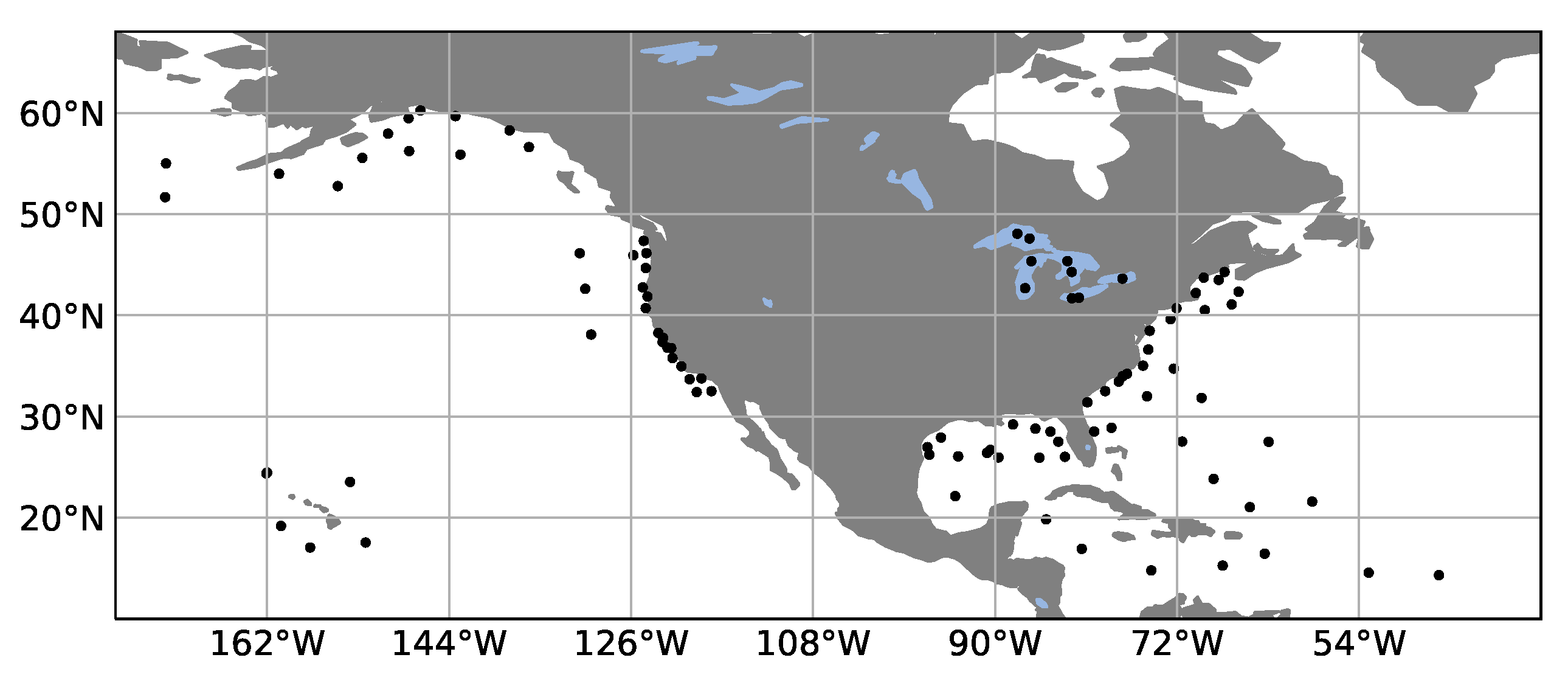
The data of Ku-band radar for 2017–2019 were collocated with the data on wind speed from 157 NDBC (National Data Buoy Center) buoys located in Atlantic and Pacific oceans, and in the Great lakes. The locations of the buoys are shown in Figure 2.
Standard meteorological wind speed product was used. It provides wind speed, wave parameters, air and water temperature every 30 min. The anemometers on buoys are installed at different heights, further wind speed was calculated at a standard height of 10 m and provided the neutral stability boundary layer. To satisfy this condition, the data for close values of air and water temperatures were taken into account so that T a i r T w a t e r < 5 ° . Wind speed at 10 m is calculated using the logarithmic wind speed profile as follows:
U 10 = U z κ 2 C d ln 1 z z 0 ,
where κ is the von Kármán constant, which is approximately 0.4, C d is the drag coefficient and z 0 is the roughness length. In this work, C d = 1.2 × 10 3 and z 0 = 9.7 × 10 5 m are used.

3. Wind Speed Retrieval Algorithm

3.1. Data around Buoys

Equivalent NRCS at nadir from PR was collocated with buoy data so that the distance between buoy and NRCS spot does not exceed 25 km, and the time gap was less than 15 min. The block of cells around each buoy is analyzed in order to exclude outliers and nonuniform wave conditions. The procedure from [24] was used to assess the quality of the data.
(1) If the circle area around the buoy contain less than 10 points, it is discarded.
(2) Individual values in the circle are marked as outliers based on median absolute deviation (MAD). The MAD is defined as:
M A D = b median { | x i M n | } ,
where M n = median { x i } and x i is the original observation in which i = 1 , 2 , 3 , n , n is the number of elements in the circle. The value of b is given as 1.4826, which is the scaling factor of Gaussian distribution. A theshold value of 3 has been used. All values outside the following criterion were removed as outliers. The criterion is given by:
x i M n M A D < 3 .
(3) The ratio R = σ σ 0 ( c i r c l e ) / σ 0 ¯ ( c i r c l e ) was considered, where σ σ 0 ( c i r c l e ) is the standard deviation and σ 0 ¯ ( c i r c l e ) is the mean of the block inside the circle. This ratio indicates the degree of NRCS inhomogeneity in the block, and if R > 0.5 , the entire block is discarded.
After this procedure, some circles were removed, the remaining circles were cleared of outliers, and σ 0 was averaged in each circle. The array of pairs ( σ 0 , U 10 ) was used to build the model for wind speed retrieval.
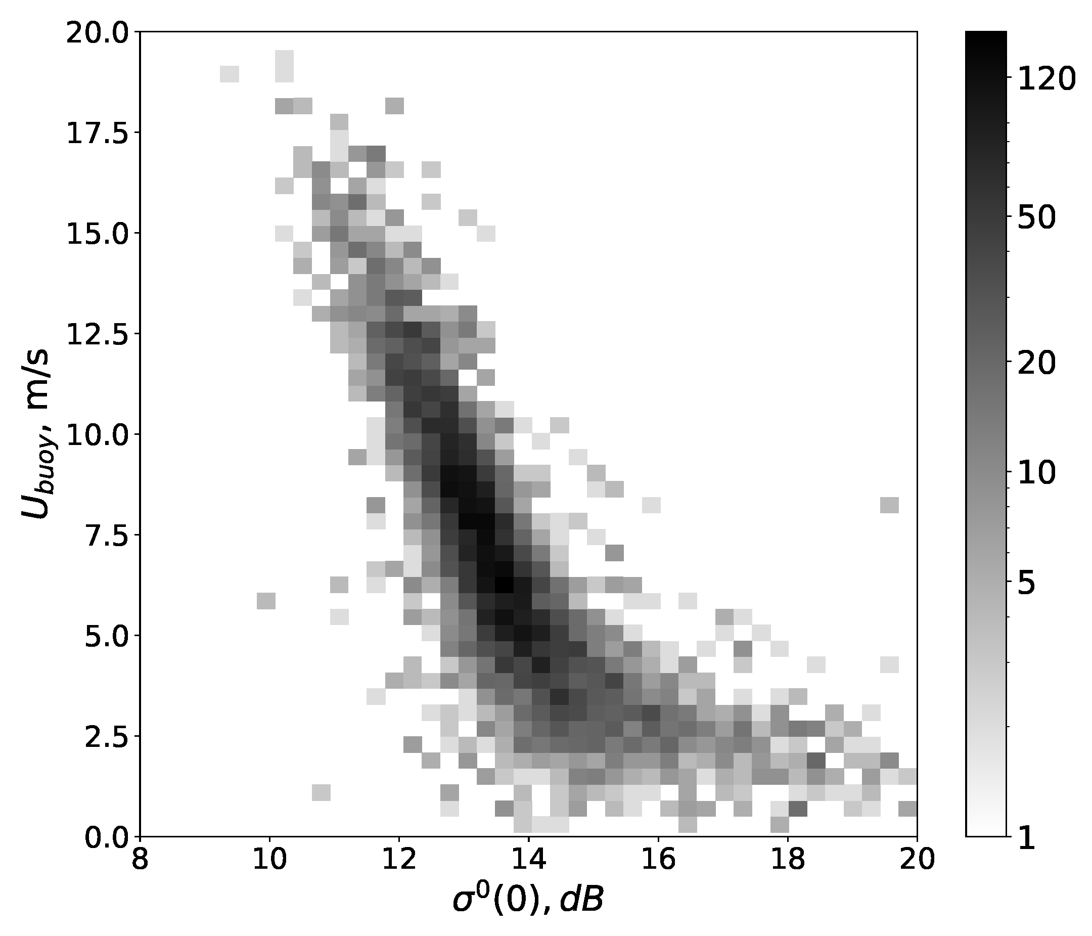
In Figure 3, the histogram of averaged values in each circle σ 0 and U 10 is presented for the Ku-band. These data will be used to build the model function U 10 ( σ 0 ) . The array contains 9634 points. Let us call this array ( σ 0 , U 10 ) L1 array.

3.2. Regression Model for Wind Speed of NRCS at Nadir

L1 array was randomly divided by half into training and validation set. In this subsection the model was obtained using the training set.
It should be noted that radar and buoy data suffer from various kinds of errors. NRCS values can contain speckle noise and calibration error and buoy measurements are also not perfect, especially taking into account that the assumption on stratification is the same for all the data. Assuming that measured values are normally distributed around the true one, averaging may help to get the result closer to the truth.
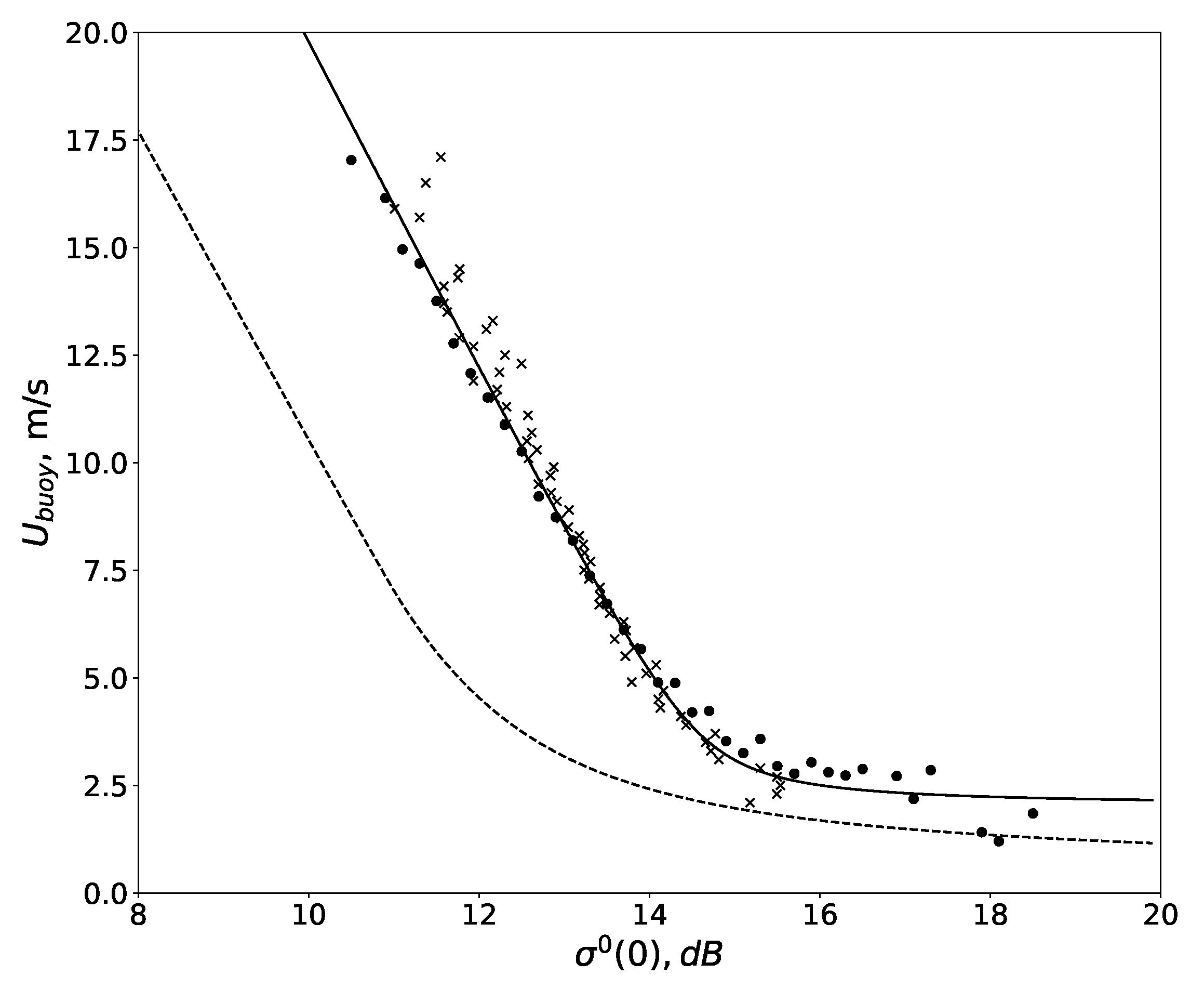
Following the procedure outlined in [7], the backscatter coefficient range was divided into bins of 0.2 dB. All collocated model U 10 values within each bin were averaged. The result is plotted as dots in Figure 4. The same binning procedure was performed for wind speed: the wind speed range was divided into bins of 0.2 m/s. The averaged NRCS within each bin is plotted as crosses. The number of collocations in the NRCS and wind speed bin is more than 10. The regression model was obtained using all averaged data.
In [7], the dependence for U 10 ( σ 0 ) consists of two parts and contains nine coefficients. We suggest the simpler continuous parameterization of the model with only four coefficients in the form:
U 10 = ( a σ 0 + b ) + ( a σ 0 + b ) 2 + c 2 + d .
The function satisfies the following requirements: it tends to a positive constant at high NRCS, has a tilted asymptote at low NRCS, the function itself and its first derivative are continuous, and its second derivative is always positive. The coefficients for Ku-band dependence are as follows: a = 1.92 , b = 28.02 , c = 1.69 , d = 2.02 . The model is valid for NRCS within 10 and 20 dB. The regression dependence for binned data is presented in Figure 4 with a solid line, and the dependence from [7] is presented with a dashed line for comparison. The model in [7] was obtained using ENVISAT (Environmental Satellite) radar altimeter data, and the discrepancy between the models is due to different calibration of the radars.

4. Discussion: Wind Speed Retrieval Accuracy

In order to assess the accuracy of the algorithm, first the validation part of the L1 array, described in Section 3.1 was used. Furthermore, the ASCAT scatterometer data was used for validation.

4.1. Comparison with Buoy

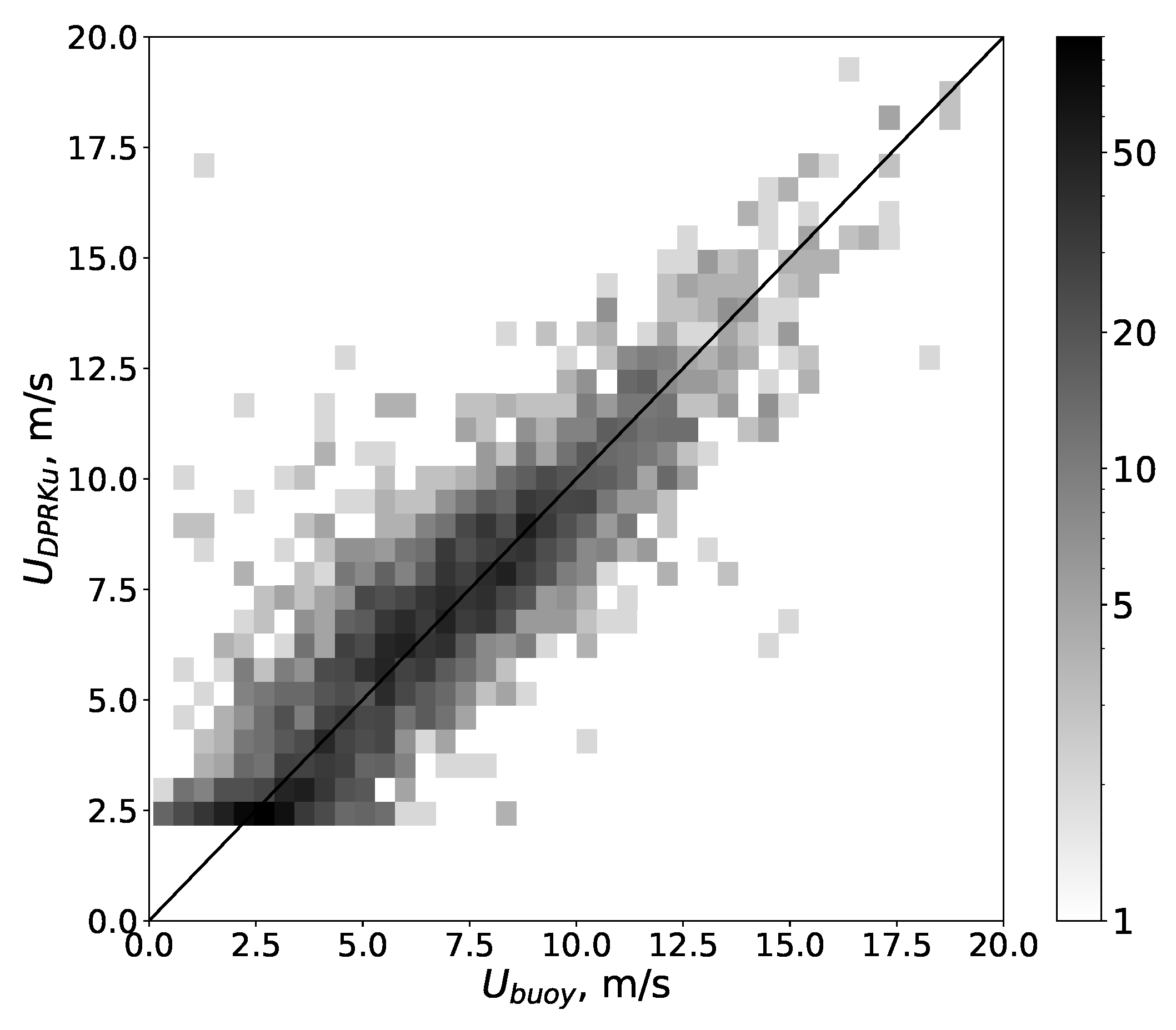
For the validation set, wind speed was calculated by (4), the resulting scatter plots are presented in Figure 5. Overall bias and standard deviation of differences (SDD) were 0.26 and 1.88 m/s, the correlation coefficient was 0.84.
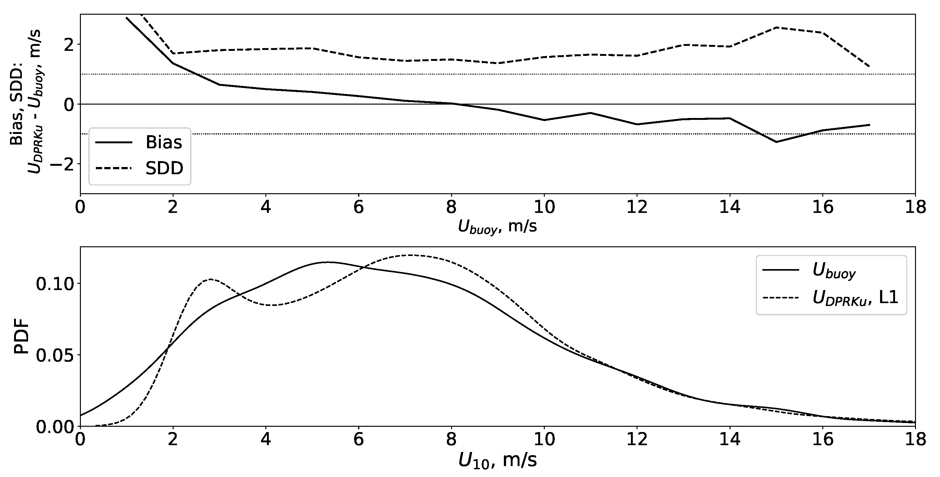
Figure 6 (top) shows the variations of bias and SDD between DPR and buoy wind speed with respect to wind speed values. The highest discrepancy is for low and high wind speeds.
The PDF of wind speeds from buoy and DPR data are in a good agreement according to Figure 6 (bottom). There is a lack of wind speeds lower than about 2 m/s in the DPR data and artificial maximum at about 3 m/s due to flat dependence of the wind speed on NRCS. This fact results in high bias and SDD for wind speeds lower than 2 m/s.

4.2. Comparison with ASCAT

Furthermore, the ASCAT-A scatterometer data was used for validation. The collocated array of ASCAT and Ku-band DPR data was formed for January 2017. Collocation length was 25 km and time was not higher than 15 min. The total array contains 57,213 pairs ( U 10 A S C A T , U 10 D P R ) . The scatter plot is presented in Figure 7. Overall bias and standard deviation of differende (SDD) were 0.28 and 1.26 m/s respectively, correlation coefficient was 0.93.
Figure 8 (top) shows the variations of bias and SDD between DPR and ASCAT wind speed with respect to wind speed values. The results of DPR are very close to ASCAT data: the binned bias is limited to 1 m/s and SDD tends to 1 m/s.
The PDF of wind speeds from ASCAT and DPR data are also in a good agreement according to Figure 8 (bottom). The lack of low wind speeds for DPR data are also observed.
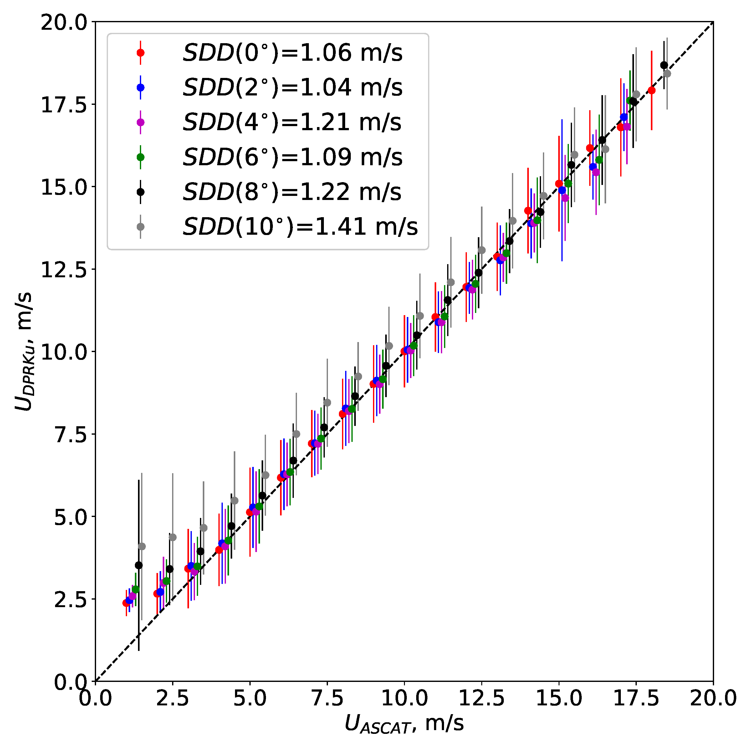
The performance of the algorithm was evaluated for different parts of the swath, corresponding to the footprints of beams with incidence angles 0 ° , 2 ° , 4 ° , 6 ° , 8 ° and 10 ° . The comparison is presented in Figure 9. The performance is quite good for all the swath, but closer to the edge of the swath, bias and SDD increase for low wind speeds.
Similar comparison was performed for SWIM data in [21], where wind speed was obtained using the GMF approach. For incidence angles 0–6 ° , both methods show good performance, but for θ 8 ° , the GMF approach error sufficiently exceeds the error of the present method, and for θ = 10 ° , the GMF method can not be applied, as was predicted in [13]. Therefore, the proposed method allows us to obtain wind speed with good accuracy in those parts of the DPR swath, where the GMF approach would not work.
In our approach, the information on the trend of σ 0 ( θ ) on a short NRCS profile was used instead of individual σ 0 values. Thus, insensitivity of NRCS to wind speed at a particular incidence angle becomes less critical. However, the accuracy of the method also degrades at the parts of the swath corresponding to the footprints of beams with incidence angles 8 ° and 10 ° .

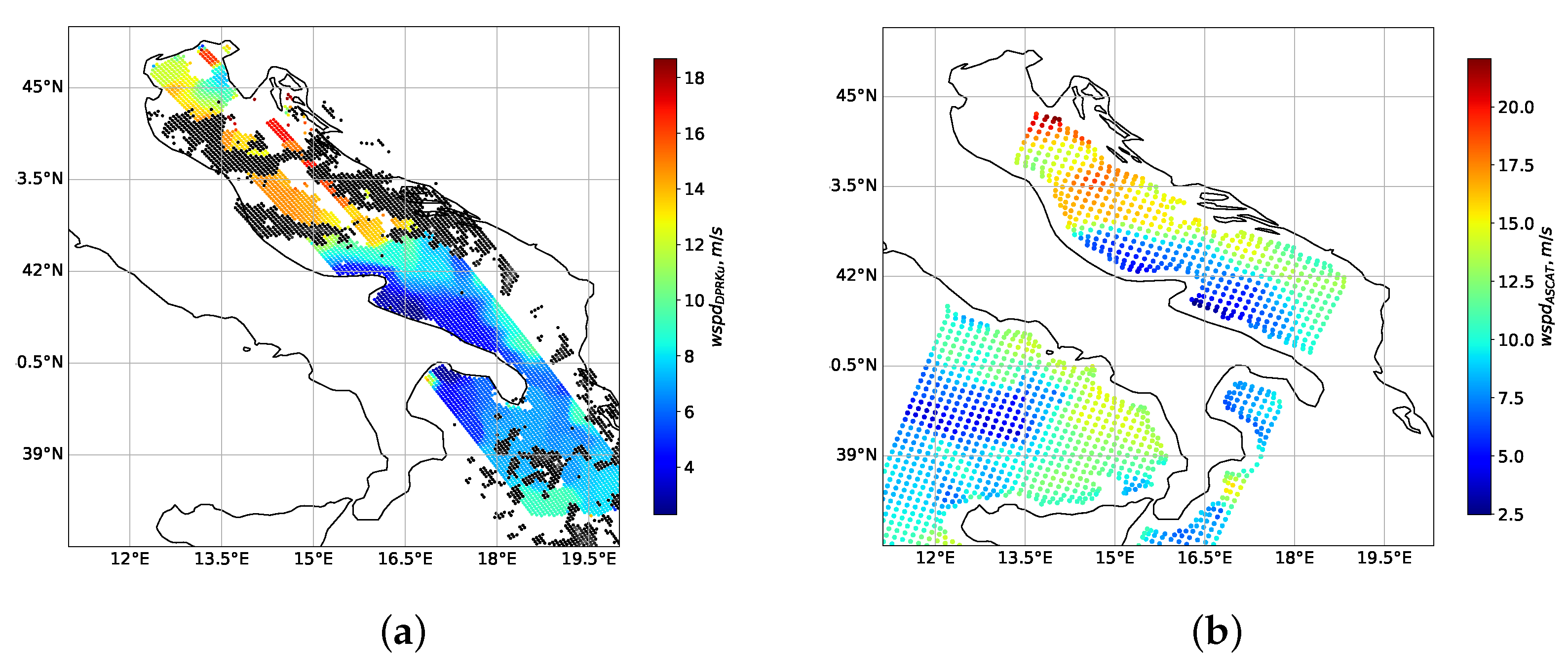
4.3. Local Case of Wind Speed Retrieval from DPR Ku-Band Radar

Let us assume applications of the algorithm to wind speed retrieval in the Adriatic sea. In winter, strong winds occur in this region. In Figure 10a, the distribution of wind speed in the Adriatic sea on 17 January 2017, 06:20 UTC, according to Ku-band DPR data, is shown in color, and rain rates over 0.5 mm/h are marked with black. The gaps are due to removal of noisy data. In Figure 10b, the wind speed distribution in the Adriatic sea on 17 January 2017, 08:50 UTC, according to ASCAT data is given, but the information on rain is absent. The sea state was stable and remained several hours, thus the data of both sensors are in a good agreement. Consecutive satellite data allow us to track the development of the atmospheric conditions.
It should be noted that DPR is able to provide the data in close proximity to the shore compared to scatterometers and altimeters. The scatterometer has a wide swath, but the resolution is lower than DPR. Coastal areas are not covered by ASCAT within about 20 km. Radar altimeters have high 5 km resolution, but it can be gained in the open sea. In fact, the altimeter antenna beam is rather wide to avoid mispointing, and the shore influences the signal within about 15 km. The advantage of DPR is a narrow beam 0 . 7 ° , thus, its data are available at about 10 km from the coast.

5. Conclusions

The algorithm for wind speed retrieval from Ku-band radar onboard a GPM satellite was developed based on buoy data. The method consists of two steps: retrieval of NRCS at nadir for a wide swath, and calculation of wind speed from the regression model. The regression model suggested in this work is simpler than in the work [7], and can be applied for obtaining wind speed from altimeter NRCS with the corresponding coefficients. The approach outlined in the paper can be further applied for wind speed retrieval from Ka-band DPR data and the data of SWIM radar onboard CFOSAT.
The advantage of the algorithm is to obtain wind speeds in a wide swath with high resolution, in close proximity to the shore, and for taking into account simultaneous information on precipitation. The accuracy of the algorithm is good according to the comparison with ASCAT scatterometer data. In the future, it is planned to perform comparisons between DPR and GMI wind speed products and to investigate the performance of the algorithm depending on the sea state.

Author Contributions

Conceptualization, M.P. and V.K.; methodology, M.P. and V.K.; software, M.P.; validation, M.P.; data curation, M.P.; writing—original draft preparation, M.P.; writing—review and editing, M.P. and V.K.; visualization, M.P. All authors have read and agreed to the published version of the manuscript.

Funding

This work is supported by RSF grant 20-17-00179.

Institutional Review Board Statement

Not applicable.

Informed Consent Statement

Not applicable.

Data Availability Statement

The buoy data on wind speed are available at https://www.ndbc.noaa.gov/ (access on 3 December 2020), DPR data were downloaded from https://storm.pps.eosdis.nasa.gov (access on 25 January 2020), ASCAT data were downloaded from https://podaac-tools.jpl.nasa.gov/ (access on 5 March 2021).

Acknowledgments

The DPR data are provided by the JAXA (JAXA Satellite Project Research (Non-Funded) PI N ER2GPN108).

Conflicts of Interest

The authors declare no conflict of interest.

Abbreviations

The following abbreviations are used in this manuscript:
ASCATAdvanced Scatterometer
DPRDual Frequency Precipitation Radar
ENVISATEnvironmental Satellite
GMIGPM Microwave Imager
GPMGlobal Precipitation Measurement
mssMean square slope
NDBCNational Data Buoy Center
NRCSNormalized Radar Cross-section
PDFProbability Density Function
TRMMTropical Raifall Measurement Mission
UTCCoordinated Universal Time

Appendix A

The simple model for NRCS dependence on incidence angle obtained within the GO (geometrical optics) approximation [23] is used. According to this model NRCS is proportional to the slope PDF. As shown in [25], slope PDF is very close to Gaussian and explicitly depends on slope mean square slope (mss). As discussed in [12], due to the diffraction effects, only a part of sea wave spectrum with wavelengths higher than radar wavelength contribute to the backscattered signal. Thus, the NRCS dependence on incidence angle includes the “radar filtered” mss. The slope PDF was regarded as Gaussian, the correlation between slopes in the two perpendicular directions was neglected. For the problem of determining σ 0 0 , these assumptions are correct, as shown in [17].
Within the frameworks of the above assumptions NRCS depends on incidence angle as follows:
σ 0 θ = | R e f f 0 | 2 cos 4 θ exp tan 2 θ 2 σ x 2 2 σ x 2 σ y 2 ,
where | R e f f θ | 2 is the effective reflection coefficient, θ is the angle of incidence, σ x 2 and σ y 2 are radar filtered mss along X and Y, respectively, where X is the direction of scanning and Y is a perpendicular direction. From (A1) NRCS at nadir, it can be directly obtained at θ = 0 as:
σ 0 0 = | R e f f 0 | 2 2 σ x 2 σ y 2 ,
hence,
σ 0 θ = σ 0 0 cos 4 θ exp tan 2 θ 2 σ x 2 .
This model is valid for incidence angles lower than at least 12 ° , where the contribution of Bragg backscatering mechanism is negligible [13]. The whole Ku-band swath contains 49 cells, but the data for 12.5– 18 ° is discarded. Only the central part of the swath is used for the cells from 9th to 41st. The method for NRCS at nadir in a wide swath calculation from DR data is discussed in detail in [17]. The steps of data processing focusing on obtaining of σ 0 0 in the swath can be briefly summarized as follows.
1. Around each cell, the square window 5 × 5 cells is considered. The cells 9, 10 and 40, 41 across the swath can not be the centers of the window, but are used in the processing of the data in windows around the 11th and 39th cells.
2. In each window the cells labeled as land, ice or precipitation are removed. At the same time each window should contain at least four different incidence angles and at least four measurements at each angle. Otherwise the window is discarded.
3. NRCS is obtained in the middle of each window using linear regression:
(a) Equation (A3) is linearized as follows:
ln σ 0 ( θ ) cos 4 θ = ln σ 0 ( 0 ) tan 2 ( θ ) / 2 σ x 2 .
(b) QC is performed to prove linear dependence between tan 2 θ and ln σ 0 cos 4 θ . The correlation coefficient is calculated as follows:
K = ln σ 0 cos 4 θ ln σ 0 cos 4 θ ¯ tan 2 θ tan 2 θ ¯ ln σ 0 cos 4 θ ln σ 0 cos 4 θ ¯ 2 tan 2 θ tan 2 θ ¯ 2 ,
where the top dash denotes averaging within the window. If K 0.7 , σ 0 ( 0 ) can be retrieved in the window. Otherwise the window is discarded.
(c) σ 0 0 is derived from the intercept term of linear regression:
ln σ 0 ( θ ) cos 4 θ = A + B tan 2 ( θ ) , σ 0 ( 0 ) = exp ( A ) .
In this work, Huber regression [26] robust to outliers was performed.
4. In cells 24, 25, 26 the value of σ 0 ( 0 ) are not calculated but are taken from raw data at −0.7, 0.1 and 0.7, respectively.
5. Median filtering of the swath was performed. According to QC steps in 2 and 3b, the swath σ 0 ( 0 ) contains gaps. The swaths of retrieved σ 0 0 was filtered by the window of 5 × 5 cells. In the midpoint of the window, the value of σ 0 0 was replaced (if the value was defined there) or filled (if there was a gap) by the median value of all the defined values within the window if their quantity exceeded a half of the total amount of cells in the window (for window 5 × 5 cells the threshold is 13). If the defined cells occupied less than a half of the window, the value or the gap remained.

References

  1. Ye, H.; Li, J.; Li, B.; Liu, J.; Tang, D.; Chen, W.; Yang, H.; Zhou, F.; Zhang, R.; Wang, S.; et al. Evaluation of CFOSAT Scatterometer Wind Data in Global Oceans. Remote Sens. 2021, 13, 1926. [Google Scholar] [CrossRef]
  2. Bourassa, M.A.; Meissner, T.; Cerovecki, I.; Chang, P.S.; Dong, X.; De Chiara, G.; Donlon, C.; Dukhovskoy, D.S.; Elya, J.; Fore, A.; et al. Remotely Sensed Winds and Wind Stresses for Marine Forecasting and Ocean Modeling. Front. Mar. Sci. 2019, 6, 443. [Google Scholar] [CrossRef] [Green Version]
  3. Hersbach, H.; Stoffelen, A.; Haan, S. An improved C-band scatterometer ocean geophysical model function: CMOD5. J. Geophys. Res. Ocean. 2007, 112, C03006. [Google Scholar] [CrossRef]
  4. Witter, D.L.; Chelton, D. A geosat altimeter wind speed algorithm and a method for altimeter wind speed algorithm development. J. Geophys. Res. 1991, 96, 8853–8860. [Google Scholar] [CrossRef]
  5. Gourrion, J.; Vandemark, D.; Bailey, S.; Chapron, B.; Gommenginger, C.P.; Challenor, P.G.; Srokosz, M.A. A Two-Parameter Wind Speed Algorithm for Ku-Band Altimeters. J. Atmos. Ocean. Technol. 2002, 19, 2030–2048. [Google Scholar] [CrossRef]
  6. Karaev, V.Y.; Kanevsky, M.B.; Balandina, G.N.; Cotton, P.D.; Challenor, P.G.; Gommenginger, C.P.; Srokosz, M.A. On the problem of the near ocean surface wind speed retrieval by radar altimeter: A two-parameter algorithm. Int. J. Remote Sens. 2002, 23, 3263–3283. [Google Scholar] [CrossRef]
  7. Abdalla, S. Ku-Band Radar Altimeter Surface Wind Speed Algorithm. Mar. Geod. 2012, 35, 276–298. [Google Scholar] [CrossRef] [Green Version]
  8. Hauser, D.; Tourain, C.; Hermozo, L.; Alraddawi, D.; Aouf, L.; Chapron, B.; Dalphinet, A.; Delaye, L.; Dalila, M.; Dormy, E.; et al. New Observations From the SWIM Radar On-Board CFOSAT: Instrument Validation and Ocean Wave Measurement Assessment. IEEE Trans. Geosci. Remote Sens. 2021, 59, 5–26. [Google Scholar] [CrossRef]
  9. Meissner, T.; Wentz, F. The Emissivity of the Ocean Surface Between 6 and 90 GHz Over a Large Range of Wind Speeds and Earth Incidence Angles. IEEE Trans. Geosci. Remote Sens. 2012, 50, 3004–3026. [Google Scholar] [CrossRef]
  10. Gao, J.; Tang, G.; Hong, Y. Similarities and Improvements of GPM Dual-Frequency Precipitation Radar (DPR) upon TRMM Precipitation Radar (PR) in Global Precipitation Rate Estimation, Type Classification and Vertical Profiling. Remote Sens. 2017, 9, 1142. [Google Scholar] [CrossRef] [Green Version]
  11. Kummerow, C.; Barnes, W.; Kozu, T.; Shiue, J.; Simpson, J. The Tropical Rainfall Measuring Mission (TRMM) Sensor Package. J. Atmos. Ocean. Technol. 1998, 15, 809–817. [Google Scholar] [CrossRef]
  12. Freilich, M.H.; Vanhoff, B.A. The Relationship between Winds, Surface Roughness, and Radar Backscatter at Low Incidence Angles from TRMM Precipitation Radar Measurements. J. Atmos. Ocean. Technol. 2003, 20, 549–562. [Google Scholar] [CrossRef]
  13. Chu, X.; He, Y.; Karaev, V.Y. Relationships Between Ku-Band Radar Backscatter and Integrated Wind and Wave Parameters at Low Incidence Angles. IEEE Trans. Geosci. Remote Sens. 2012, 50, 4599–4609. [Google Scholar] [CrossRef]
  14. Chu, X.; He, Y.; Chen, G. Asymmetry and Anisotropy of Microwave Backscatter at Low Incidence Angles. IEEE Trans. Geosci. Remote Sens. 2012, 50, 4014–4024. [Google Scholar] [CrossRef]
  15. Chen, P.; Zheng, G.; Hauser, D.; Xu, F. Quasi-Gaussian probability density function of sea wave slopes from near nadir Ku-band radar observations. Remote Sens. Environ. 2018, 217, 86–100. [Google Scholar] [CrossRef]
  16. Hossan, A.; Jones, W.L. Ku- and Ka-Band Ocean Surface Radar Backscatter Model Functions at Low-Incidence Angles Using Full-Swath GPM DPR Data. Remote Sens. 2021, 13, 1569. [Google Scholar] [CrossRef]
  17. Panfilova, M.A.; Karaev, V.Y.; Guo, J. Oil Slick Observation at Low Incidence Angles in Ku-Band. J. Geophys. Res. Ocean. 2018, 123, 1924–1936. [Google Scholar] [CrossRef]
  18. Li, L.; Im, E.; Connor, L.; Chang, P. Retrieving ocean surface wind speed from the TRMM Precipitation Radar measurements. IEEE Trans. Geosci. Remote Sens. 2004, 42, 1271–1282. [Google Scholar] [CrossRef]
  19. Ren, L.; Yang, J.; Zheng, G.; Wang, J. Wind speed retrieval from Ku-band Tropical Rainfall Mapping Mission precipitation radar data at low incidence angles. J. Appl. Remote Sens. 2016, 10, 1–14. [Google Scholar] [CrossRef]
  20. Bao, Q.; Zhang, Y.; Lang, S.; Lin, M.; Gong, P. Sea Surface Wind Speed Inversion Using the Low Incident NRCS Measured by TRMM Precipitation Radar. IEEE J. Sel. Top. Appl. Earth Obs. Remote Sens. 2016, 9, 5262–5271. [Google Scholar] [CrossRef]
  21. Ren, L.; Yang, J.; Xu, Y.; Zhang, Y.; Zheng, G.; Wang, J.; Dai, J.; Jiang, C. Ocean Surface Wind Speed Dependence and Retrieval From Off-Nadir CFOSAT SWIM Data. Earth Space Sci. 2021, 8, e2020EA001505. [Google Scholar] [CrossRef]
  22. Barrick, D. Rough Surface Scattering Based on the Specular Point Theory. IEEE Trans. Antennas Propag. 1968, 16, 449–454. [Google Scholar] [CrossRef]
  23. Bass, F.; Fuks, I. (Eds.) Chapter 7—Scattering from Large-Scale Roughness. In Wave Scattering from Statistically Rough Surfaces: International Series in Natural Philosophy; Pergamon Press: Oxford, UK, 1979; Volume 93, pp. 220–315. [Google Scholar]
  24. Ribal, A.; Young, I.R. 33 years of globally calibrated wave height and wind speed data based on altimeter observations. Sci. Data 2019, 6, 1–15. [Google Scholar]
  25. Cox, C.; Munk, W. Measurement of the Roughness of the Sea Surface from Photographs of the Sun’s Glitter. J. Opt. Soc. Am. 1954, 44, 838–850. [Google Scholar] [CrossRef]
  26. Huber, P.; Ronchetti, E. Robust Statistics; J. Wiley, Cop.(Wiley Series in Probability and Statistics); Wiley: Hoboken, NJ, USA, 2009; p. 384. [Google Scholar]
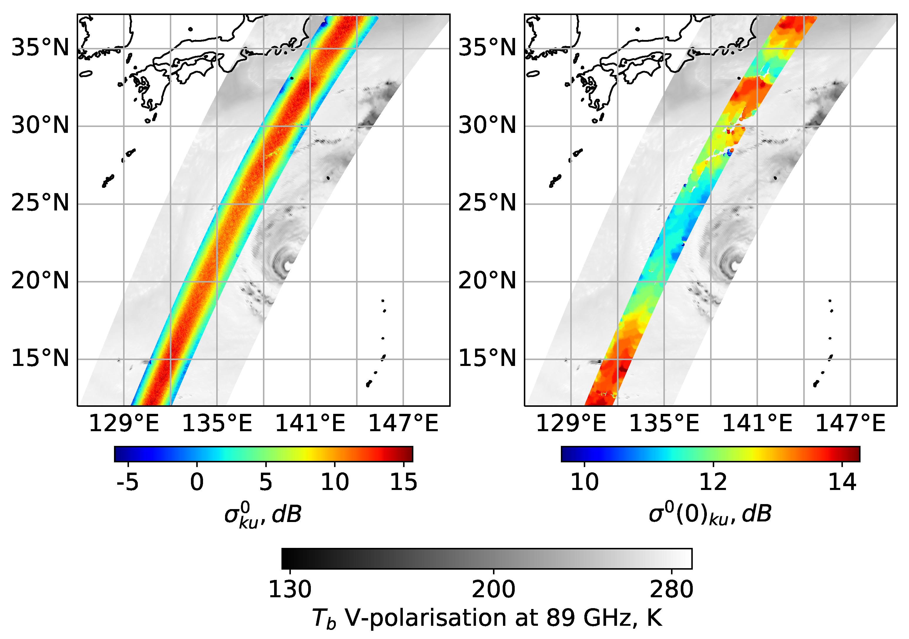
Figure 1. Raw data of Ku-band radar (left) and retrieved NRCS at nadir (right) over the image of brightness temperature from GMI data at 89 GHz, V-polarization. The track passes over the typhoon Hagibis at 09:40 GMT on 9 October 2019.
Remotesensing 13 04565 g001
Figure 2. NDBC buoy data used in the analysis.
Remotesensing 13 04565 g002
Figure 3. Histogram of wind speed dependence on NRCS.
Remotesensing 13 04565 g003
Figure 4. Wind speed from NDBC buoys dependent on NRCS at nadir. Dots correspond to averaged wind speed at a given NRCS, crosses correspond to averaged NRCS at a given wind speed. The solid line is the regression dependence for (4), the dashed line is the dependence from [7].
Remotesensing 13 04565 g004
Figure 5. Global comparison between Ku-band radar and buoy wind speed values during the period 2017–2019.
Remotesensing 13 04565 g005
Figure 6. Wind speed difference (bias) and standard deviation of the difference (SDD) between DPR Ku-band radar and NDBC buoys (top). Wind speed PDF for DPR and buoy data of L1 array (bottom).
Remotesensing 13 04565 g006
Figure 7. Global comparison between Ku-band radar and ASCAT wind speed values during January 2017.
Remotesensing 13 04565 g007
Figure 8. Wind speed difference (bias) and standard deviation of the difference (SDD) between DPR Ku-band radar and ASCAT (top). Wind speed PDF for DPR and ASCAT validation array (bottom).
Remotesensing 13 04565 g008
Figure 9. Wind speed comparison between DPR winds and collocated ASCAT winds for different parts of the swath, corresponding to the footprints of beam with incidence angles 0 ° , 2 ° , 4 ° , 6 ° , 8 ° and 10 ° .
Remotesensing 13 04565 g009
Figure 10. (a) Wind speed in the Adriatic sea on 17 January 2017, 06:20 UTC, according to Ku-band DPR data (color), rain contaminates cells with rain rate over 0.5 mm/h (black); (b) wind speed in the Adriatic sea on 17 January 2017, 08:50 UTC, according to ASCAT data.
Remotesensing 13 04565 g010
Publisher’s Note: MDPI stays neutral with regard to jurisdictional claims in published maps and institutional affiliations.