An Investigation on Seasonal and Diurnal Cycles of TOA Shortwave Radiations from DSCOVR/EPIC, CERES, MERRA-2, and ERA5

Abstract

Reflected shortwave (SW) solar radiations at the top of atmosphere from Clouds and the Earth’s Radiant Energy System (CERES), Modern Era-Retrospective analysis for Research and Applications version 2 (MERRA-2), and ECMWF Reanalysis 5th Generation (ERA5) are examined to better understand their differences in spatial and temporal variations (seasonal and diurnal cycle timescale) with respect to the observations from the Earth Polychromatic Imaging Camera (EPIC) on the Deep Space Climate Observatory (DSCOVR) satellite. Comparisons between two reanalyses (MERRA-2 and ERA5) and EPIC reveal that MERRA-2 has a generally larger deviation from EPIC than ERA5 in terms of the SW radiance and diurnal variability in all seasons, which can be attributed to larger cloud biases in MERRA-2. MERRA-2 produces more ice/liquid water content than ERA5 over the tropical warm pool, leading to positive SW biases in cloud and radiance, while both reanalyses underestimate the observed SW radiance from EPIC in the stratus-topped region off the western coast of US/Mexico in the boreal summer. Himalaya/Tibet region in the boreal spring/summer and the midlatitude Southern Hemisphere in the boreal winter are the regions where MERRA-2 and ERA5 deviate largely from EPIC, but their deviations have the opposite sign. Vertical structures of cloud ice/liquid water content explain reasonably well these contrasting differences between the two reanalyses. As two independent observations, CERES and EPIC agree well with each other in terms of the SW radiance maps, showing 2–3% mean absolute errors over the tropical midlatitudes. The CERES-EPIC consistency further confirms that the reanalyses still have challenges in representing the SW flux and its global distribution. In the CERES-EPIC observation differences, CERES slightly overestimates the diurnal cycle (as a function of local solar time) of the observed EPIC irradiance in the morning and underestimates it in the afternoon, while the opposite is the case in the reanalyses.

1. Introduction

The reanalysis models have been producing the top of atmosphere (TOA) radiative fluxes over the last several decades to advance our understanding of the Earth’s energy balance [1,2,3,4,5,6,7,8]. There have been considerable improvements in data assimilation techniques and satellite observations to produce realistic radiative fluxes, but deficiencies in the reanalysis models still prevent them from accurately representing the TOA radiation fluxes, especially the reflected shortwave (SW) flux. Evaluations of radiative energy from two widely used recent reanalyses, Modern Era-Retrospective analysis for Research and Applications version 2 (MERRA-2) [7] and ECMWF Reanalysis 5th Generation (ERA5) [8], and many coupled models reveal that the bias of upward radiative flux is largely from the SW, while the longwave (LW) (i.e., outgoing LW radiation (OLR)) is in relatively better agreement with the observations [9,10]. The MERRA-2 has reduced the bias of the net TOA radiative energy from MERRA through significant improvement in OLR, but little improvement has been made for the reflected SW energy at the TOA [11]. It is important in climate models to identify and quantify how much of the solar radiation is absorbed by the atmosphere and reflected by clouds and other high-albedo surfaces [12]. In addition, further improvements are needed for a more accurate representation of the upward SW flux in the models. This has been a great challenge, since uncertainties of the TOA radiative energy in the reanalysis can be induced not only by data assimilation techniques [13,14], but also by deficiencies in model radiation schemes [15,16] and cloud schemes [17,18] that compute the radiative fluxes and cloud properties from the assimilated dynamical and thermodynamic structures.

Despite recent advances in the reflected TOA SW flux observations, the remote sensing of SW fluxes from space is still a great challenge. MERRA-2’s all-sky reflected SW flux at TOA over the period 2001–15 is found to be ~7 W m⁻² higher [19] than that from Clouds and the Earth’s Radiant Energy System (CERES) Energy Balanced and Filled (EBAF) [20,21], resulting in a net TOA flux imbalance of ~4 W m⁻². On a regional scale, there are positive/negative biases of cloudiness in MERRA-2 that may cause this globally averaged TOA flux imbalance. For instance, MERRA-2 ice clouds are overestimated over the tropical ocean and extratropical ocean in the Southern Hemisphere (SH), while the clouds are generally underestimated in the marine stratocumulus areas such as the western coast of United States (US)/Mexico [19]. It is also identified that excessive cloud cooling or high albedo occurs in the western Pacific and Southern Ocean (SO) [11]. This overrepresentation of SW cloud forcing is particularly dominant, resulting in more global mean energy leaving the Earth than in satellite-based observation, while the cloudiness over northern midlatitudes (especially over continents) is improved over MERRA.

ERA5 tends to have a better representation of the TOA SW flux at a higher model resolution (a quarter-degree horizontal grid spacing), through a series of upgrades made from the radiation and cloud scheme used by ERA-Interim reanalysis [22] with ~80 km horizontal resolution. Although the global mean energy budgets are improved over ERA-Interim, there is still underestimated annual mean TOA net radiation and net energy loss of the atmosphere from ERA5 [8]. Accurate simulation of cloud and radiative processes remains challenging, especially over tropical deep convective regions, stratocumulus regions in the subtropics, midlatitude oceans, and polar regions [10], where MERRA-2 has similar kinds of problems.

Many previous studies evaluated the radiative fluxes from reanalysis by comparing them with satellite radiative fluxes provided by the CERES EBAF project [19,23,24]. CERES radiative fluxes at TOA are estimated by converting radiance measurements based upon angular distribution models (ADMs) that consider the angular dependence of the Earth’s radiation [25,26]. This angular dependence is associated with the scene type including surface type, cloud fraction, cloud/aerosol optical depth, cloud phase, etc., as well as the illumination angle. Although the CERES radiative fluxes provide a reasonable estimation of the TOA SW fluxes, the CERES ADMs are obtained from the monthly statistics at a fixed local time. Thus, the ADM-based approach may be limited by complex terrains and clouds in the effort to resolve the 3D radiative fluxes and global energy balance at TOA [27]. Uncertainties in TOA fluxes can be caused by changes in accompanying images and errors in cloud properties [27,28] and aerosol optical depths [29]. The number of daytime measurements is also limited: they are collected only two local times a day.

The reanalysis model deficiencies and limitations of CERES products described above motivate us to assess the MERRA-2 and ERA5 capability and the CERES measurement uncertainty using independent datasets, for representing the TOA SW radiation. One of the independent observation datasets is the SW radiances from the Earth Polychromatic Imaging Camera (EPIC) on the Deep Space Climate Observatory (DSCOVR) satellite [30]. The DSCOVR orbit is at the unique vantage point, the Sun–Earth Lagrange-1 (L-1) point, where the satellite can view the reflected SW radiances 12–23 times in a day. Compared to CERES, the EPIC measurements have a full local time coverage, with data production at higher resolution globally (e.g., 2048 × 2048 number of pixel rows and columns with ~8 km resolution at the center of the Earth disc). The EPIC measures the Earth’s radiances in 10 spectral channels [30,31]. It was found, in a regression analysis, that the radiances from three EPIC channels could adequately represent the CERES SW flux and its variabilities [27]. We utilize all EPIC spectral bands, however, to more accurately quantify the spatial and temporal variations of the TOA SW radiances/fluxes estimated from CERES and the reanalyses.

In this study, we first convert the TOA upward SW fluxes from CERES and reanalyses to the SW radiances at each solid angle in the EPIC view. We then regress the 10-channel EPIC radiances onto these estimated radiances from CERES, MERRA-2, and ERA5, separately, to obtain the broadband EPIC TOA SW radiances that best match the spatial distributions of the SW radiances from CERES and two reanalyses in each season. Smaller regression residual indicates a more consistent spatial distribution between two datasets. Thus, our regression analysis is focused on the spatial and temporal variations of the regressed radiances and regression residuals that could represent the SW radiance errors in CERES and reanalyses. A particular focus is placed on relating the regional SW radiance errors identified from regression residuals to cloud fraction biases in reanalyses. It is widely recognized that cloud fraction plays a critical role in the radiative transfer model of reanalysis to minimize the radiative flux biases [14,32]. In our assessment, we investigate the role of cloud fraction for the regional differences in radiance errors between two reanalyses.

The paper is organized as follows. Section 2 introduces satellite-based observations and two reanalysis products used in this study. Methodology for conversion of upward SW flux to radiance based on the Lambertian assumption, and the multiple regression of 10-channel EPIC radiances, are described in Section 3. Section 4 explores the upward SW fluxes and radiances from CERES and two reanalyses to compare their seasonal distributions and diurnal cycles with those from EPIC, followed by discussion of radiance errors in relation to cloud biases in Section 5, and conclusions are given in Section 6.

2. Satellite-Based Observations and Reanalysis Data

2.1. EPIC

The Earth Polychromatic Imaging Camera (EPIC) is one of the main instruments on board NOAA’s Deep Space Climate Observatory (DSCOVR) deep space satellite launched in 2015 [30]. DSCOVR is located at the Earth–Sun L-1 point, ~1.5 × 10⁶ km away from Earth at the gravity neutral point that allows DSCOVR to hover between the Sun and Earth. The major role of the EPIC is to take images of the nearly-complete sunlit side of Earth to provide insight into Earth’s energy balance and monitor cloud properties (e.g., reflectivity, height, and phase), ozone and aerosol levels, properties of vegetation and land, and UV radiation estimates at Earth’s surface. EPIC has 10 narrowband channels (see yellow rectangles in Figure 1 with the wavelength range from 317 through 780 nm, all producing high resolution images of the Earth disc on a 2048 × 2048 pixel detector [31]. Note that the solar reference spectrum in Figure 1 is from Total and Spectral Solar Irradiance Sensor-1 (TSIS-1) solar spectral measurement [33]. Approximately half of the solar energy is in the spectrum with wavelengths <780 nm and the EPIC’s roughly hourly sampling of the reflected SW flux in this spectral range provides a unique dataset to characterize and understand the diurnal variation of the TOA SW. In this study, we examine the Earth’s SW radiance (monthly and hourly) that EPIC measures for the year 2017. To obtain the narrowband EPIC radiances for 2017, the EPIC measured photon counts are first converted to reflectance using the calibration coefficients developed based on comparisons with MODIS Aqua and Terra L1B 1 km reflectance [34]. Radiance at the EPIC instrument is then estimated from reflectance by weighting band average flux at each channel and EPIC viewing zenith angle. We also use EPIC cloud fraction [35] in this study. Monthly mean cloud fractions are compared with distribution of errors in SW radiances from two reanalyses to discuss their relationship.

2.2. CERES

CERES is a series of instruments from a low-Earth orbiting (LEO) satellite to measure outgoing LW and reflected SW radiation at TOA [20,25]. The CERES standard products also provide cloud properties to improve understanding of the cloud impact on the Earth’s energy budget, climate, and weather. In this study, the upward SW flux at TOA from CERES SYN1deg hourly data and the estimated SW radiance (1° longitude × 1° latitude resolution) projected onto the EPIC observing point (i.e., L-1) in 2017 are examined on a seasonal and diurnal cycle timescale basis to compare with those from two selected reanalyses (MERRA-2 and ERA5).

2.3. Reanalysis Dataset: MERRA-2 and ERA5

The upward SW flux at TOA and cloud ice/liquid water content available from two reanalyses, MERRA-2 [7,36,37] and ERA5 [8], are investigated to assess the performance of the reanalysis model in representing the global Earth radiation and understand how significantly the discrepancy in the Earth’s reflected SW radiations between reanalyses and observation is attributable to limitation of cloud representation in reanalysis models. Horizontal resolution of these two data is 0.625° longitude × 0.5° latitude for MERRA-2 and 0.25° longitude × 0.25° latitude for ERA5. For the radiative transfer model that is crucial to determine the radiative fluxes, MERRA-2 uses the Community Radiative Transfer Model (CRTM) [38] version 2.1.3 to assimilate all satellite radiances [11]. ERA5 uses the Radiative Transfer for TOVS version 11 (RTTOVv11) model [39] with which the partly all-sky assimilation is performed, as opposed to the clear-sky assimilation in ERA-Interim.

3. Methodology

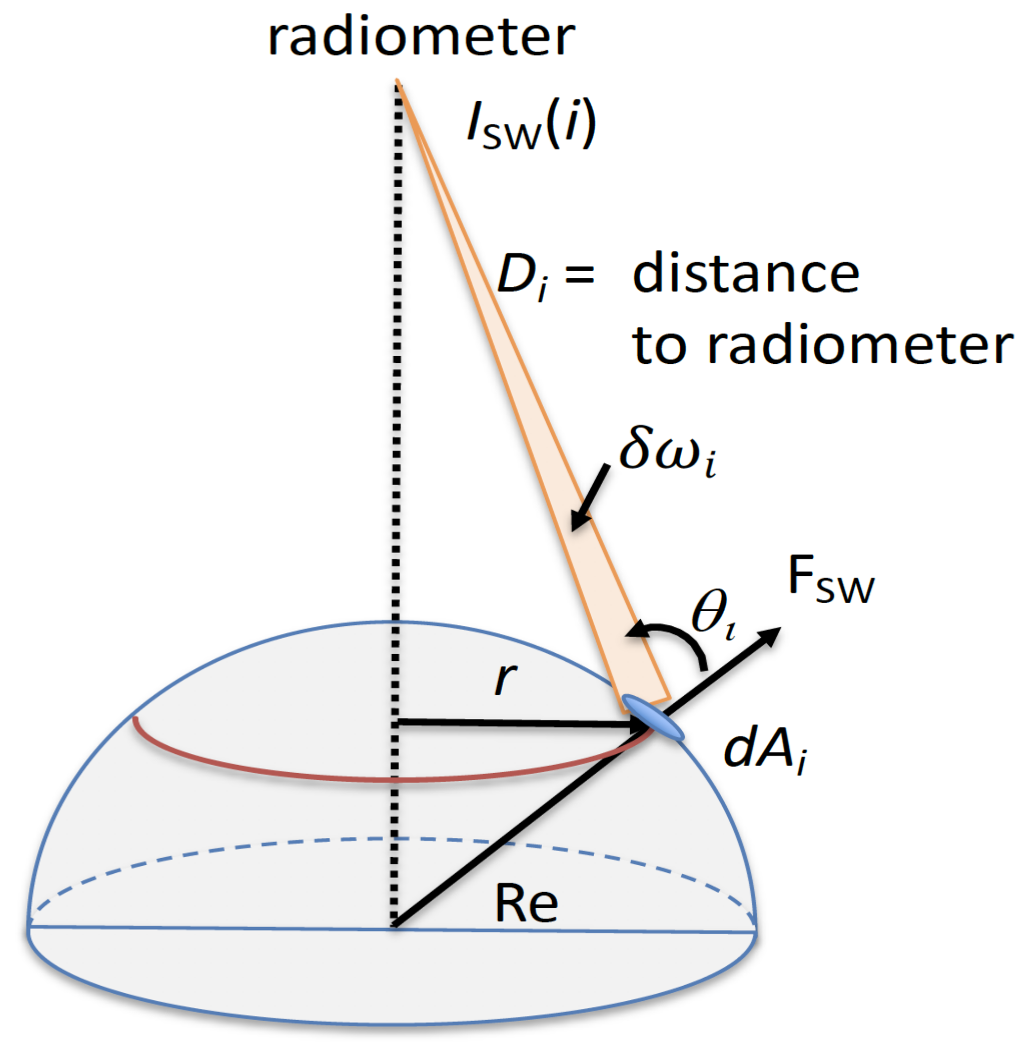
3.1. Conversion of the Upward Shortwave Flux to Radiance

Because the direction of upward SW fluxes from CERES and two reanalyses is normal to the Earth’s surface, we convert them to make their direction identical to narrowband EPIC radiances from 10 channels prior to regressions described in Section 3.2. We assume the Lambertian reflection for Earth’s surface. Although it may not be a perfect assumption, this method is shown to be still effective to understand the SW radiance errors due to reanalysis model deficiencies associated with cloud representations (see Section 4 and Section 5 for details). In addition, the EPIC’s geolocation information is used to take into account the temporal variation of angle (θ) and distance (D) between Earth and EPIC.

The radiance observed by a radiometer at the L-1 point (e.g., DSCOVR) is given by

$$I_{sw}\left(i\right)={\frac{F_{sw}\left(i\right)}{\pi }}_{ }cos{\theta }_i\delta {\omega }_i$$

(1)

$$\delta {\omega }_i=\frac{d{A}_{i}cos{\theta }_i}{D_i^2}$$

(2)

where dA_i is the area of radiation on Earth to radiometer, $\delta {\omega }_i$ is the solid angle of dA_i to radiometer, θ is the angle between radiometer and Earth’s surface normal, F_sw(i) is the TOA upward SW flux at location (i), I_sw(i) is the Earth’s radiance at location (i), and D_i is the distance of dA_i to radiometer. The unit of the I_sw(i) is W/m²/sr, while the unit of F_sw(i) is W/m². The order of magnitude of I_sw(i) is much smaller than F_sw(i) due to $\raisebox{1ex}{$d{A}_i$}\!\left/ \!\raisebox{-1ex}{$D_i^2$}\right.$ factor. Figure 2 illustrates how I_sw(i) is physically related to F_sw(i) based on the Lambertian assumption.

While Earth’s radiances at each location (i) provide horizontal distribution, one needs to integrate all the radiances at each surface location (i) to obtain the Earth irradiance.

$$IR{R}_{sw}=\int \frac{F_{sw}\left(i\right)}{\pi D_i^2}co{s}^2{\theta }_{i}d{A}_i$$

(3)

3.2. Multiple Regression

Multiple regression is used to achieve the best fit for the radiances measured by ten EPIC channels from the radiance field estimated from MERRA-2, ERA5, and CERES for each season. Fitting with smaller residual (regression error) on a global basis indicates a more consistent spatial distribution between two datasets. In this study, we perform the pairwise regression between EPIC and other datasets to produce a quantitative assessment of the TOA SW radiances reported in these data. Before regression, we regrid the EPIC radiance fields onto the spatial resolution of target field. We then set the radiance (I_sw(i)) from MERRA-2, ERA5, or CERES described in Section 3.1 to be predictand and the regridded EPIC radiances from individual 10 channels to be predictors.

$$I_{sw}\left(i\right)=r_0+r_1{E}_1\left(i\right)+r_2{E}_2\left(i\right)+r_3{E}_3\left(i\right)+\cdots +r_{10}{E}_{10}\left(i\right)+ϵ\left(i\right)$$

(4)

where $r_0$ is the interception and $r_1\dots r_{10}$ are regression coefficients from EPIC radiances for each channel ($E_1\dots E_{10}$). From the residuals between target field and regressed field, we assess the consistency of each product (CERES and two reanalyses) in representing the spatial distribution of the broadband EPIC radiances. Because EPIC and CERES are independent observations of the TOA radiances, their differences may be viewed as the observation uncertainty, whereas the differences between EPIC/CERES and MERRA-2/ERA5 may be considered as the observation–model differences. In this study, we focus on the observation–model differences with an amplitude greater than the EPIC–CERES differences in a regional scale at the same location.

4. Results

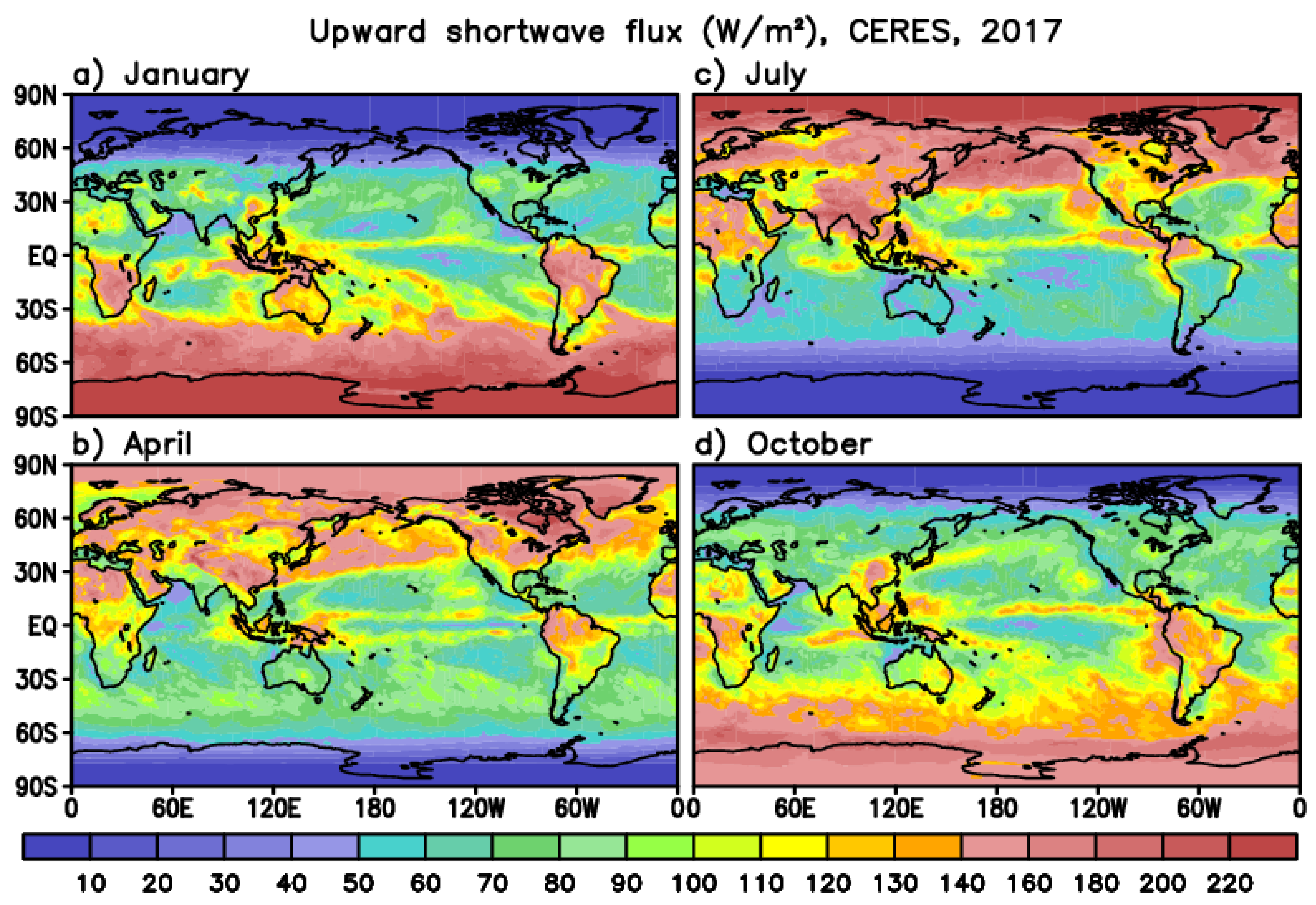
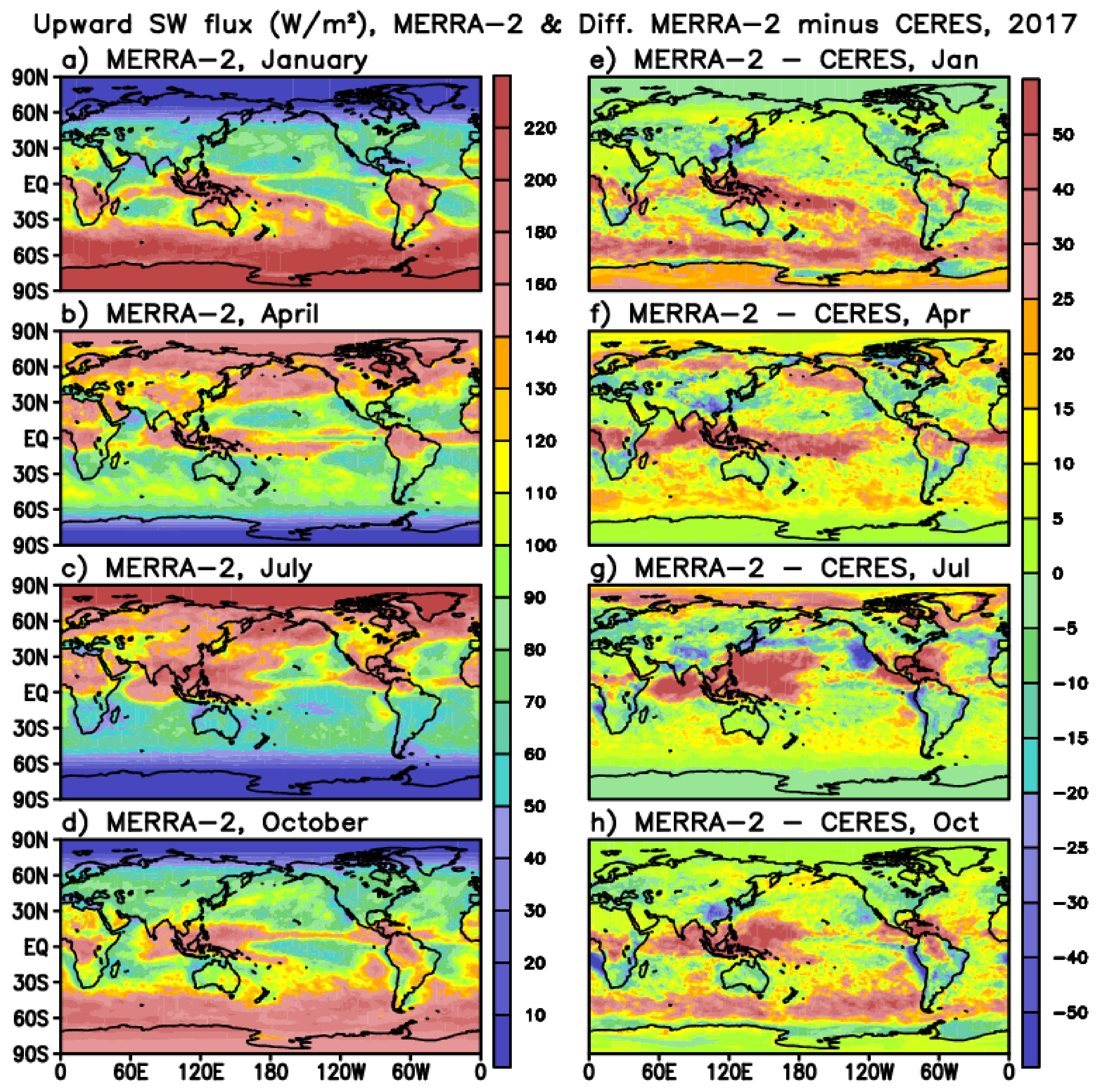
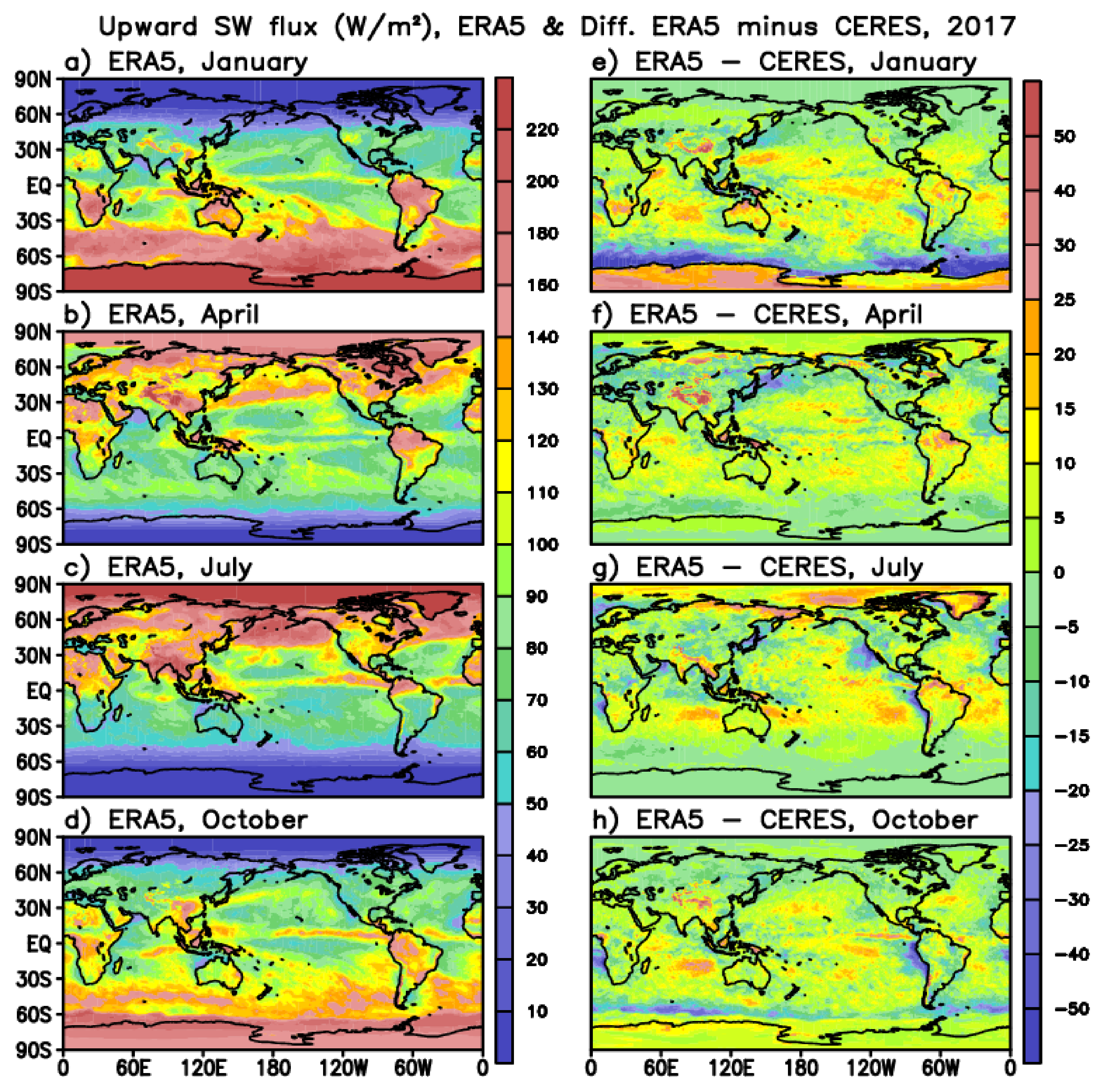
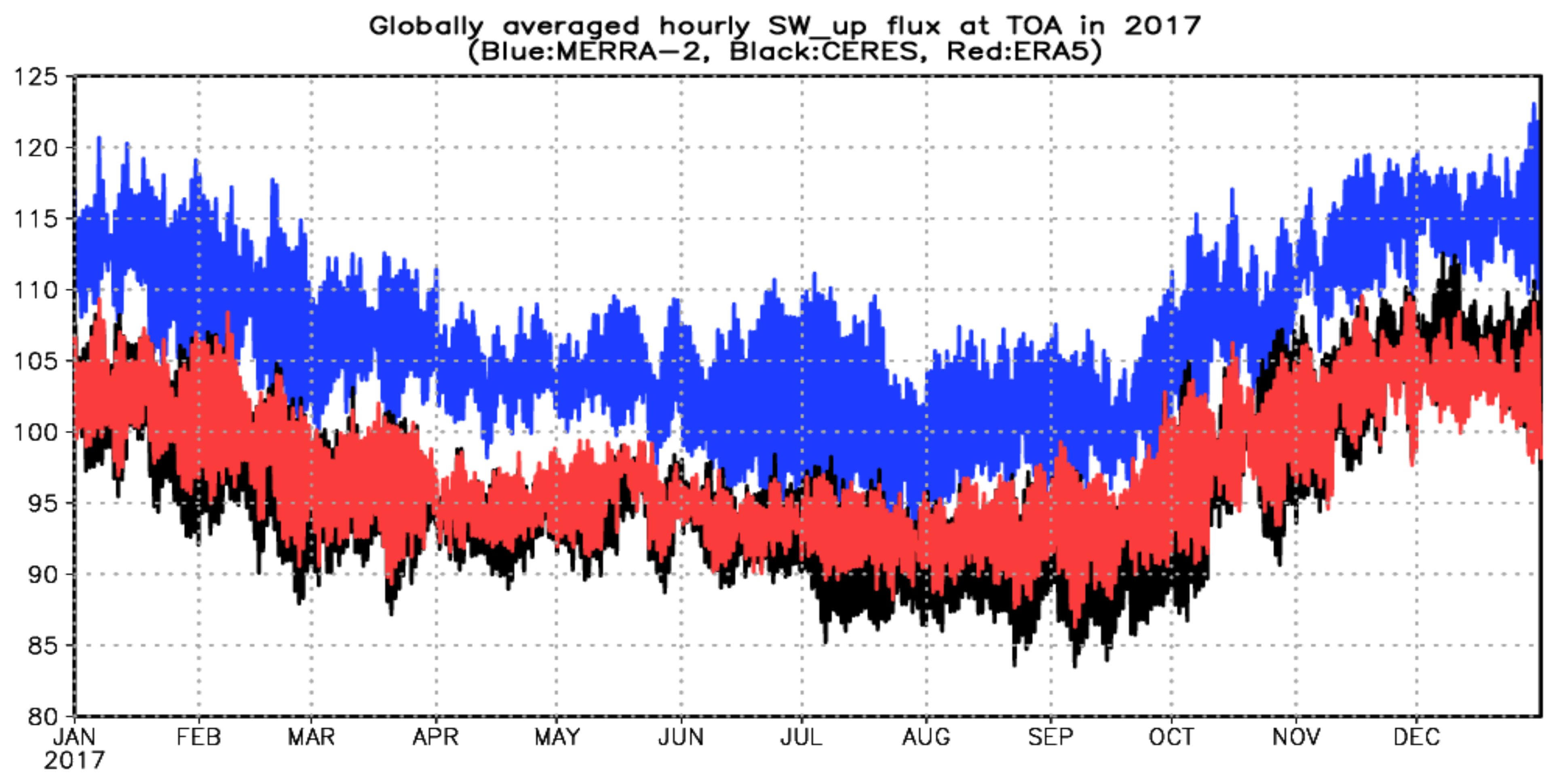
4.1. TOA Upward Shortwave Fluxes from CERES, MERRA-2, and ERA5

Geographical distributions of TOA upward SW fluxes (F_sw) and their seasonal change are compared for CERES, MERRA-2, and ERA5 in 2017. Figure 3 illustrates the horizontal distribution of F_sw from CERES for January, April, July, and October, as a representation of the boreal winter, spring, summer, and fall. It is apparent that the maximum F_sw is located in Antarctica in the boreal winter (January) and in the Arctic region in the boreal summer (July). The area with high F_sw greater than 150 W m⁻² is more broadly expanded in the polar region in January than in July due to a shorter Sun–Earth distance in January. The mid-latitude region also undergoes a strong seasonal change, with the maximum F_sw in January (July) in the Southern (Northern) Hemisphere. Cloudier regions over the ocean (e.g., tropical convective region) show relatively larger F_sw than less-cloudy regions in the subtropical latitudes. The well-known low-tropospheric stratocumulus region over off the western coast of the US has the maximum F_sw in boreal summer (July) and significant reduction in the other three seasons, consistent with seasonal variation of observed stratocumulus cloud [40,41].

The capability of the reanalysis in representing the seasonal F_sw changes is evaluated by comparing the CERES F_sw with that from MERRA-2 (Figure 4) and ERA5 (Figure 5). The left panel in Figure 4 illustrates the F_sw from MERRA-2 for four different seasons. Overall seasonal change, at a glance, is quite similar to that captured from CERES shown in Figure 3. However, the difference map on the right panel clearly highlights the notable overrepresentation of the CERES F_sw by MERRA-2. The tropical western Pacific including the warm pool region has large positive differences throughout the season, with a broader overestimation across the western Pacific and Indian Ocean in July. The excessive SW cloud forcings in the reanalysis model appear responsible for the positive F_sw differences in this region [11,19] (see more detailed discussion in Section 5). Another region where the positive differences are prevalent is the SO in October and January. In contrast, the regions near the west coast of the US and Mexico, and west coast of South America and Africa [41], known to be often characterized by low clouds in the boreal summer and fall, show negative differences in general, implying the underestimation of stratocumulus by MERRA-2 in July and October.

Seasonal F_sw changes for another reanalysis (ERA5) and their comparison with CERES are presented in Figure 5. Positive difference values are distributed widely, though they are generally weak, indicating larger F_sw by ERA5 primarily over low- to mid-latitudes. There are also several local underestimations that require attention. For instance, low-cloud regions of the western coast of North and South America and Africa show negative differences in boreal summer and fall (Figure 5g,h). In addition, unlike the overestimation of CERES F_sw over the SH storm track and SO by MERRA-2, ERA5 produces significantly smaller F_sw than CERES over that region in January and October (Figure 5e,h). Another region that MERRA-2 and ERA5 exhibit opposite signs of differences is Himalaya/Tibet. While the F_sw from MERRA-2 is clearly smaller than CERES in April and July (Figure 4f,g), the opposite is true for ERA5 (Figure 5f,g).

Time evolution of globally averaged F_sw from three products is plotted in Figure 6 to quantify their average values and relative differences. It demonstrates that F_sw obtained from MERRA-2 are larger than those from ERA5 and CERES by ~10 W m⁻², which corresponds to approximately ~10% of F_sw from ERA5 and CERES. The ERA5 exhibits better agreement with CERES in terms of the magnitude of F_sw. Annual average of F_sw from each product is 106.3 W m⁻² for MERRA-2, 97.4 W m⁻² for ERA5, and 96.6 W m⁻² for CERES.

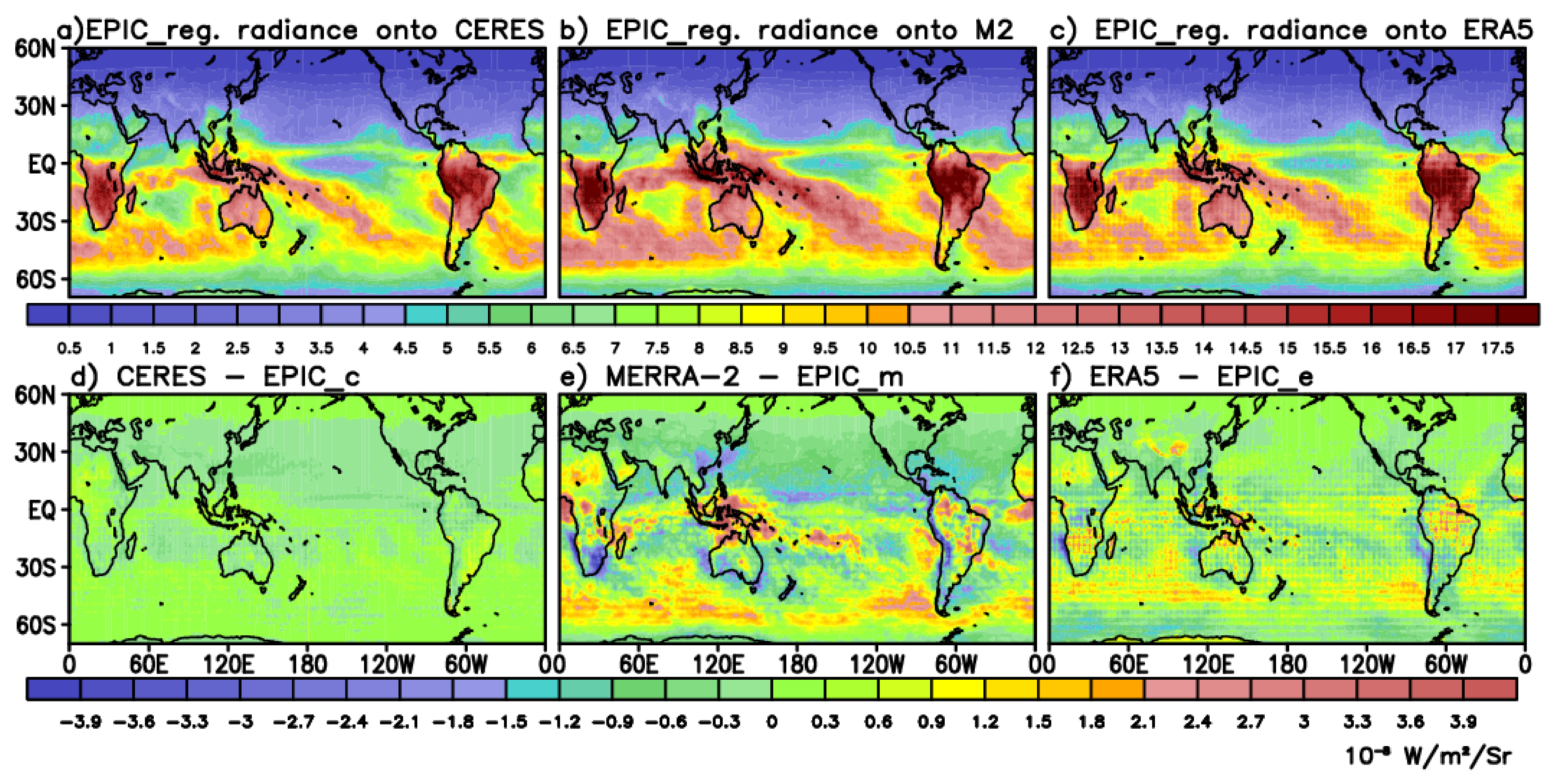
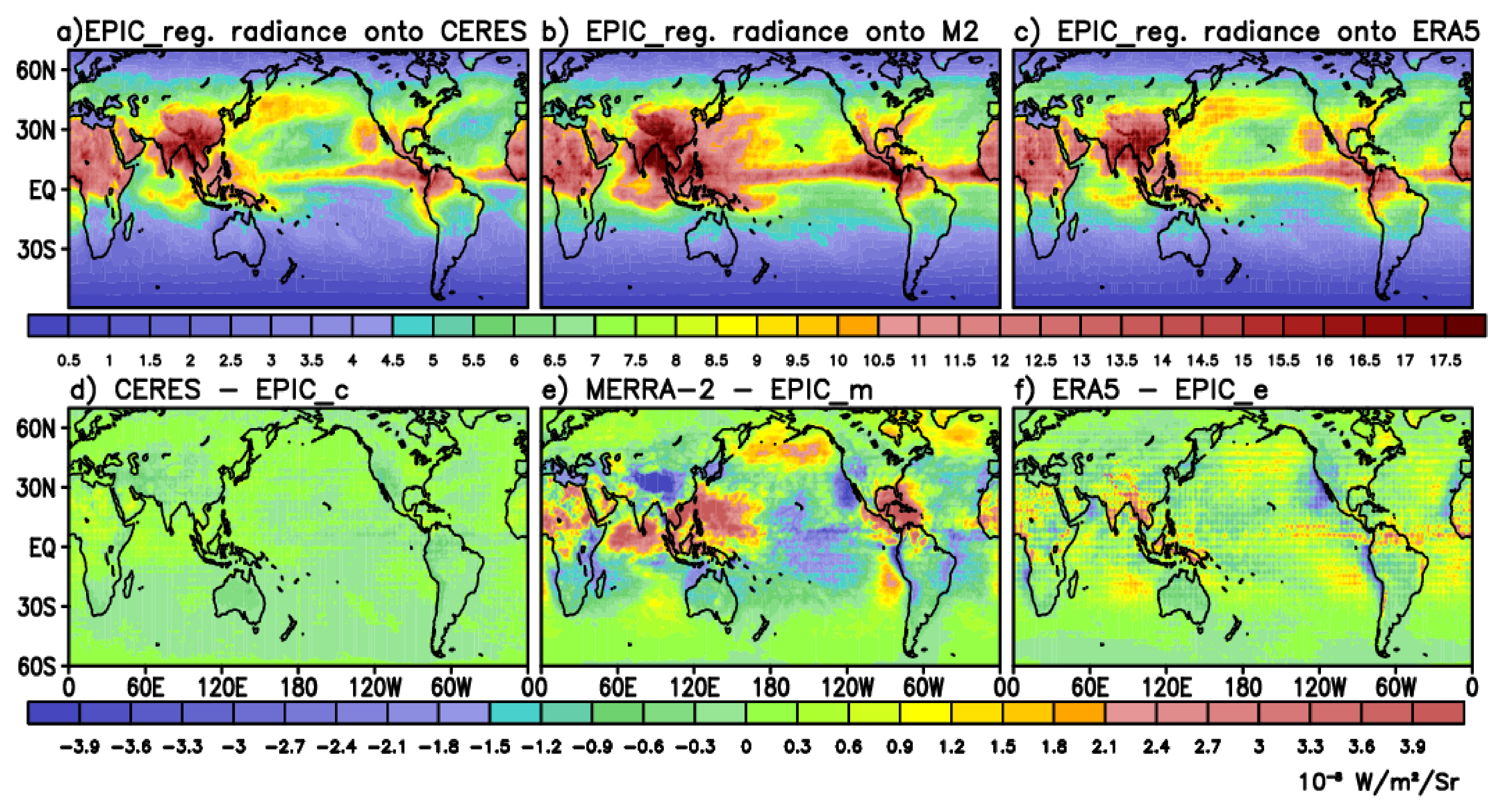
4.2. Regression of the EPIC Radiance onto CERES and Two Reanalyses

Descriptions of CERES in Section 1 suggest that even CERES can have some caveat, though CERES is believed to provide more realistic radiation values than reanalysis. To further address the fidelity of the SW radiations from CERES, MERRA-2, and ERA5, we convert their F_sw to Earth’s radiances and compare them with the EPIC observation. As described in Section 3.2, we regress the radiances measured by EPIC that consist of 10 channels onto the radiance from CERES, MERRA-2, and ERA5, respectively, to identify how reliably the radiances from these three products match well with the EPIC radiance in each season. The regression residuals (errors) can be considered as the SW radiance errors from CERES, MERRA-2, and ERA5.

Figure 7a–c exhibit the distribution of regressed EPIC radiance (no inclusion of contribution from error term in Section 3.2) onto the CERES, MERRA-2, and ERA5 radiance for boreal winter (December, January, and February). Land areas within the 0°–40°S that include southern Africa, Maritime Continent, Australia, and South America have the largest values exceeding 15 × 10⁻⁸ W m⁻² Sr⁻¹. This is associated with the southward displacement of the maximum rainfall region over land. Ocean in the SH shows regional-scale patterns of regressed radiances, while the Northern Hemisphere (NH) from 30°N to high latitudes exhibits a rather uniform distribution of small radiances not greater than 5 × 10⁻⁸ W m⁻² Sr⁻¹. The regions with larger radiance values in the SH ocean can be linked to more cloud fractions. Specifically, the South Pacific Convergence Zone (SPCZ) [42] is characterized by more convective clouds in boreal winter.

To identify how well the EPIC radiance matches with the CERES radiance, differences between the radiance converted from CERES F_sw and the regressed EPIC radiance shown in Figure 7a are plotted in Figure 7d. Difference maps demonstrate that differences are generally not greater than 1 × 10⁻⁸ W m⁻² Sr⁻¹. NH from tropics to midlatitudes (~50°N) tends to show positive differences while the negative differences are dominant in the SH. The spatial average of absolute differences between CERES and EPIC over 0°–360°E and 50°S–0°, where the highest radiances can be seen, is found to be 2.1% of the spatial average of the EPIC radiances (Figure 7a).

It is apparent that the differences in Figure 7d are globally smaller than the case for MERRA-2 (Figure 7e) and ERA5 (Figure 7f). Figure 7e (7f) is the global distribution of differences between the radiances from MERRA-2 (ERA5) and the regressed EPIC radiance onto MERRA-2 (ERA5). The positive differences from MERRA-2 are prevalent over the SH, including the SPCZ and the maximum rainfall regions over land, though some negative differences are seen on a local scale. Over the NH, it does not show regional-scale difference patterns, and differences are weakly negative across the domain. The result for ERA5 in Figure 7f reveals that positive differences prevail over SH ocean from tropics to ~45°S, consistent with the features from CERES and MERRA-2. However, the magnitude of differences is not larger than that for MERRA-2 (Figure 7e). The spatial averages of absolute differences between MERRA-2/ERA5 and EPIC are 9.7% (MERRA-2) and 7.4% (ERA5) of the spatial average of the EPIC radiances.

The same investigation is made for boreal summer (June, July, and August) to identify any seasonality in the spatial pattern of radiance differences between three products and EPIC. Regressed EPIC radiances onto CERES, MERRA-2, and ERA5 radiance in Figure 8a–c show that the region of the maximum has been shifted to the north, compared to boreal winter, spanning the land areas over the NH. The largest radiance from the regressed EPIC radiance is seen over India and Southeast Asia, the region of strong Asian summer monsoon activity. The subtropical region including Sahel in Africa and the Middle East is also characterized by large radiances. These large radiances over the cloud-free region appear to be related to the strong reflectance of incoming SW radiation at the desert surface [43]. In addition, the equatorial eastern Pacific and the southwest of the US region show larger radiances than nearby regions. Comparison of the radiances with EPIC in Figure 8d–f indicates that CERES (Figure 8d) has obviously smaller errors than MERRA-2 (Figure 8e) and ERA5 (Figure 8f). The spatial averages of absolute difference for three products over 0°–360°E and 0°–50°N are 2.6%, 15.5%, and 8.2% of the spatial average of the EPIC radiances, indicating that the performances are not better than boreal winter.

The largest positive differences for MERRA-2, with respect to EPIC, are found over the tropical western Pacific warm pool. It implies that the reanalysis model may overestimate the observed convective cloud, leading to excessive SW radiance (Figure 8e). MERRA-2 and ERA5 show opposite signs of differences that persist from boreal spring (Figure A1) over the Himalaya/Tibet region (Figure 8e,f), as it is also found from comparison of F_sw with CERES in Figure 4 and Figure 5. ERA5 shows negative difference values south of 45°S in the SH (Figure 8f) while the MERRA-2 shows positive differences (Figure 8e). It is also noteworthy that, across the Western Hemisphere, the largest magnitude of negative differences is present over the west of the US from both MERRA-2 and ERA5. They may be attributed to the poor performance of the reanalysis models in representing low-tropospheric stratus and stratocumulus in that region. An earlier study which examined the MERRA-2 indicated that MERRA-2 overestimates the observed cloud over the tropical ocean due to overestimated deep convection and extratropical ocean in the SH, while underestimates the cloud in marine stratocumulus areas such as off the western coast of US/Mexico [19].

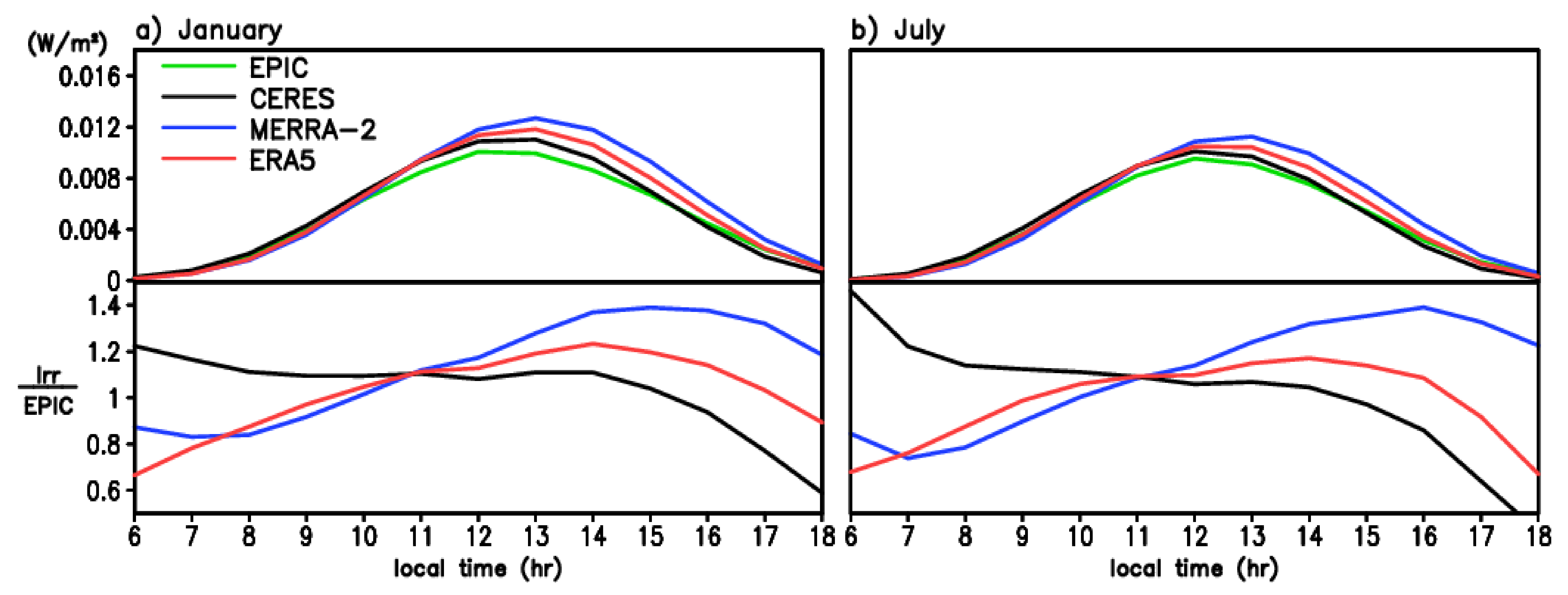
4.3. Diurnal Cycle of Earth’s Reflected Irradiance from EPIC, CERES, MERRA-2, and ERA5

In this section, we investigate shorter timescale (i.e., diurnal cycle) variation of SW radiation from EPIC, CERES, MERRA-2, and ERA5 to quantify their relative differences. Diurnal cycle of Earth’s reflected irradiance (global integral of radiance, see Section 3.1) is plotted in Figure 9 as a function of local solar time to address how realistically the CERES, MERRA-2, and ERA5 reproduce the observed peak time and shape of diurnal cycle revealed by EPIC. Diurnal cycle over the globe from EPIC clearly shows the maximum peak at noon in winter and summer (green lines) due to the high solar elevation that implies a strong solar illumination. It was also found from EPIC observations that cloud cover—a key factor in regulating reflectance—has a daily minimum around local noon [44]. While CERES (black line) produces the diurnal cycle quite close to EPIC in January, two reanalyses (blue and red lines) lag the maximum peak by an hour, along with overestimation (Figure 9a). The exaggeration of diurnal amplitude lasts through afternoon as the ratio of reanalysis irradiance to that from EPIC remains above 1 in the afternoon (lower panel in Figure 9a).

We find that the main features observed in January are still dominant in July. Both EPIC and CERES reach the maximum irradiance at noon followed by gradual decrease in the afternoon (Figure 9b). However, the irradiance at noon from reanalyses remains nearly steady (ERA5) or continues to grow by 1 p.m. (MERRA-2), displaying the ratio greater than 1 in the lower panel. Contrary to afternoon, the ratio is smaller than 1 in the morning, as seen also in January, due to underestimation of EPIC irradiance by ~20% (Figure 9b). This upward trend with time is in contrast to the downward trend identified from CERES that presents the ratio exceeding 1 in the morning and lower than 1 in the afternoon. More precisely, the ratio from CERES is closer to 1 from ~10 a.m. through 2pm than the other hours, possibly due to two CERES measurements that occur at 10:30 a.m. and 1:30 p.m. local time every day. Consistency of CERES irradiance with EPIC is relatively low beyond this time range (10 a.m.–2 p.m.), showing ratios becoming increased with time (backward) before 10 a.m., and lower than 1, and rapidly decreasing with time after 2 p.m.

Although our focus here is to examine the diurnal cycle as a function of local solar time, the diurnal cycle as a function of the Coordinated Universal Time (UTC), reported in earlier studies, has the daily maximum SW flux at 8~9 a.m. UTC, associated with highly reflective Africa near the center of the sunlit Earth disc. It was found that the upward SW fluxes from both CERES and EPIC reach the maximum at 8 a.m. UTC, with the CERES values generally being larger than EPIC during the UTC daytime hours [45].

5. Discussion

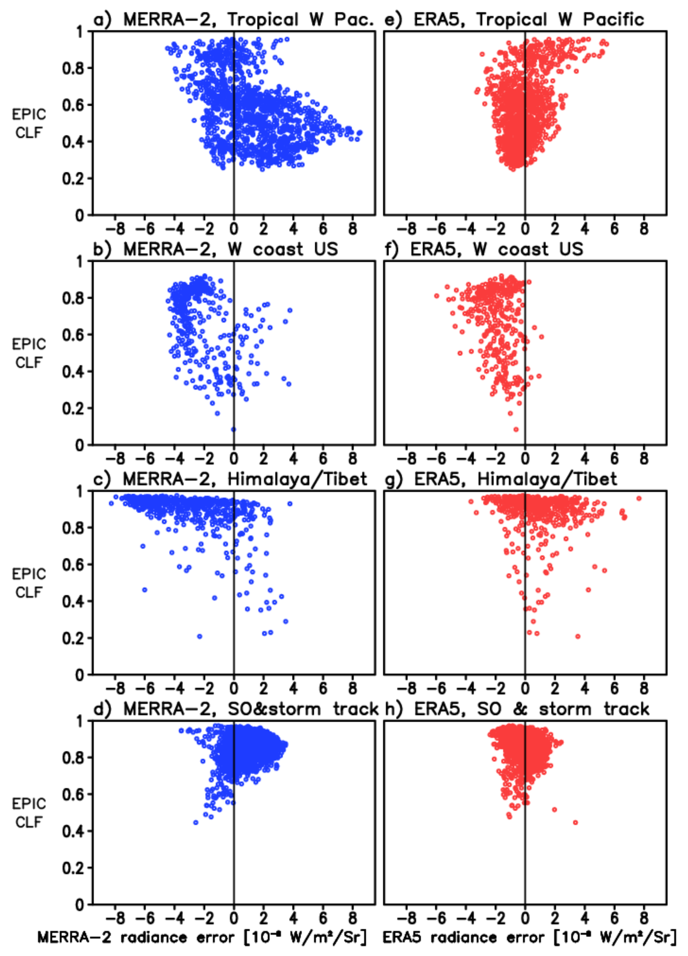
5.1. Radiance Errors versus Observed Cloud Fraction

The radiance errors from two reanalyses may be caused by the model deficiency in representing the observed cloud fraction, based on the understanding of major contributions of cloud fractional coverage and its diurnal variation to SW radiation [46]. Figure 10 compares the reanalyses’ radiance errors (Figure 7 and Figure 8) with the observed cloud fractions obtained from EPIC. Several regions are selected for investigation, including the tropical western Pacific (warm pool), low-cloud region over off the western coast of US and Mexico, Himalaya/Tibet, and SH midlatitudes (storm track and SO). The warm pool is where the positive radiance errors (Figure 7 and Figure 8) are dominant in MERRA-2, while the low-cloud region has the negative errors in both MERRA-2 and ERA5. The last two regions are where the radiance errors from MERRA-2 and ERA5 have opposite signs.

Scatter plots in the upper panel of Figure 10 explain clearly that each reanalysis (x-axis) has the unique relationship with the EPIC cloud fraction (y-axis) in boreal summer over the tropical western Pacific. The main feature is that the large positive errors from ERA5 tend to be found where cloud fractions are above ~0.8 (Figure 10e), but MERRA-2 does not display these large radiance errors over cloud-dense areas (Figure 10a). The largest positive errors from MERRA-2 are found over cloud fraction range of 0.3 to 0.6. This contrasting feature indicates that improvement of positive radiance differences between ERA5 and EPIC is required specifically in the areas of large cloud fraction, while the improvement for MERRA-2 is critical over areas that have the medium level of cloud fractions (0.3–0.6).

The low-cloud region over off the western coast of US/Mexico reveals quite different scatter plot distributions, compared to the tropical western Pacific. The distribution in Figure 10b,f clearly indicates a negative relationship of radiance errors with the observed cloud fractions due to underestimation of low cloud in the reanalysis model [47]: negative radiance errors with large amplitude are found over the high fractional cloud coverage area while the amplitude of error is small over the low fractional coverage area. The result reveals that the realistic representation of clouds in reanalysis models to reduce the negative radiance errors in this region is more particularly required over cloud-dense areas for both reanalyses.

Himalaya/Tibet is the most elevated region in the world and the Tibetan Plateau is especially known to be a heat source in summer, substantially affecting the Asian summer monsoon and climate [48,49,50]. The results for the Himalaya/Tibet region in Figure 10c,g indicate that the observed cloud fractions are generally high, exceeding 0.8 on the majority of grid points. MERRA-2 is characterized more by negative radiance errors, while the opposite is true for ERA5. The high fractional cloud coverages (greater than 0.8) are distributed across the entire range of amplitude in these radiance errors, and the largest amplitudes of positive (negative) radiance errors are found over the area of observed cloud fractions greater than 0.9 for ERA (MERRA-2) (Figure 10c,g). As shown in detail in Figure 11c, the ERA5 may need a decrease in cloud liquid water content at low- to mid-troposphere to reduce this positive radiance errors, while MERRA-2 needs improvement of underestimated cloud liquid water content to decrease the amplitude of negative radiance errors in this region.

The SH midlatitudes that include the storm track and SO are shown to be cloudy, having the cloud fractions greater than ~0.5 (Figure 10d,h). Positive (negative) radiance errors with large (small) cloud fraction are seen from MERRA-2, but that relationship is not clear in ERA5. For MERRA-2, positive radiance error is somewhat more dominant than negative error (Figure 10d), while ERA5 exhibits opposite features (Figure 10h). This contradiction appears associated with significant difference in vertical structure of cloud liquid water content between two reanalyses (e.g., Figure 11d), and overestimation of low cloud in MERRA-2 over this region [19]. We further examine these different characteristics in the next section.

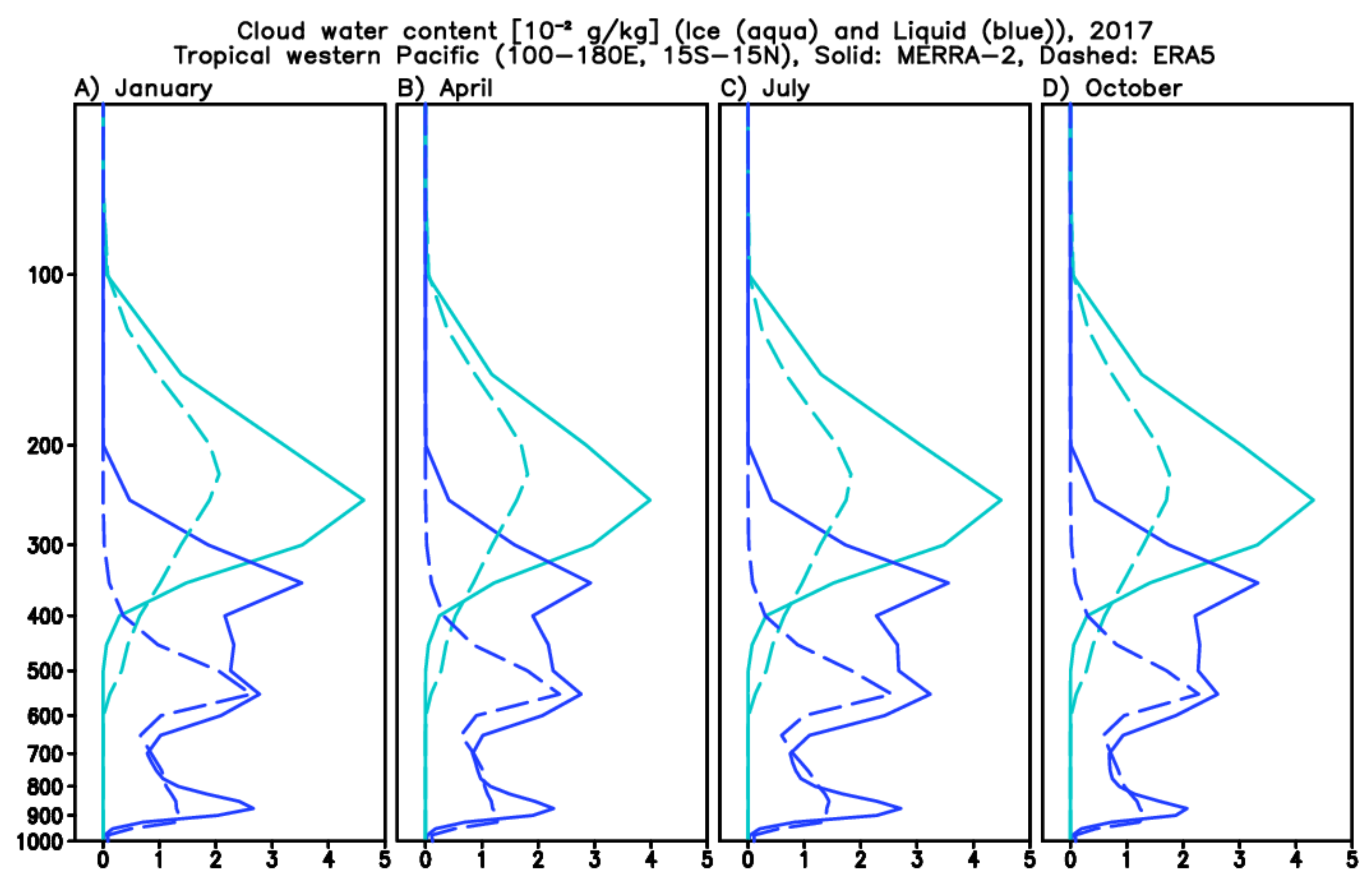
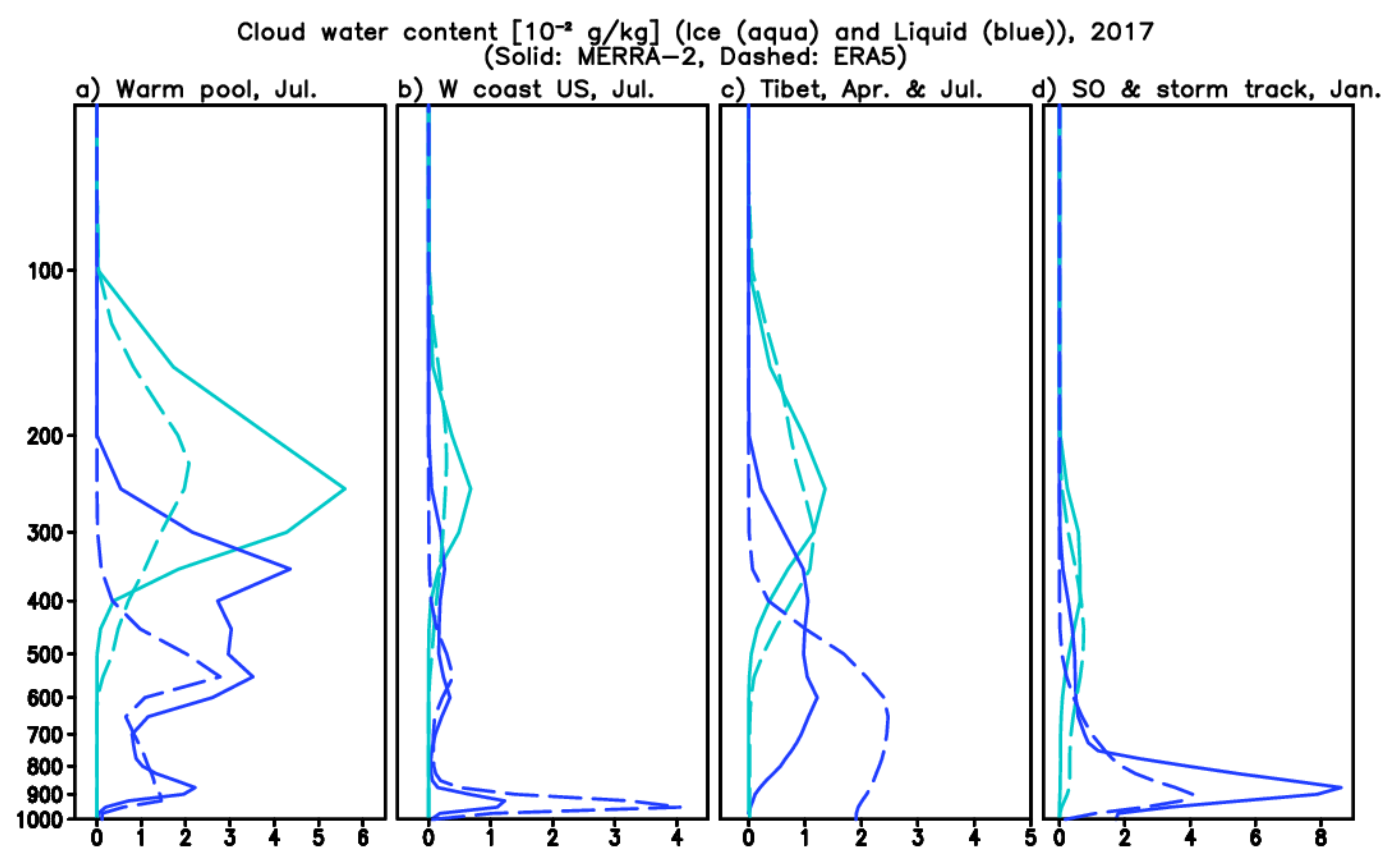
5.2. Vertical Structure of Cloud Ice/Liquid Water Contents from Reanalyses

Different vertical structures of cloud ice/liquid water content from two reanalyses, for the regions selected in Section 5.1, offer some good insights into the close relationship between the SW radiance error and ice/liquid water content, which is a prerequisite for cloud formation. Vertical profiles over the tropical western Pacific (warm pool) in Figure 11a demonstrate that both ice and liquid water content from MERRA-2 are manifestly more than those from ERA5. The largest difference in ice water content is at ~250 hPa, the level of maximum ice water content for both reanalyses. Liquid water content profile indicates the conspicuous difference (more than tripled) at pressure levels of 300−400 hPa, while the difference rapidly decreases from mid- (500 hPa) to low-troposphere. The overall structure is in line with a larger overestimation of Earth’s reflected SW radiance by MERRA-2 in this region. Higher cloud water content at upper troposphere in MERRA-2 than in ERA5 can yield excessive cloud cooling and reflectance to solar insolation, resulting in a higher modeled upward SW flux than observed in this region [11]. ERA5 is shown to have a mix of positive and negative radiance errors, as it is shown earlier in Figure 7, and the magnitude of error is smaller than that for MERRA-2. We also find that the main features from these vertical profiles (Figure 11a) in two reanalyses lasts through the other seasons (Figure A2).

Over off the western coast of US and Mexico, Figure 11b indicates that the largest difference between two reanalyses is pronounced at low-tropospheric 900−1000 hPa pressure levels, where liquid water content from ERA5 is almost three times as much as that from MERRA-2. Difference in ice water content at the upper troposphere is rather small, as the deep convective activity is not typically vibrant in this region [41]. Lack of low-level water content from MERRA-2 indicates that the process involving low-level cloud (e.g., stratus and stratocumulus) formation is weak in the reanalysis model, leading to significantly larger negative error in radiance (Figure 8c) and underestimation of low cloud [19]. As for ERA5, it is not clear yet why we still see the presence of negative radiance errors (Figure 8d), although the low-level liquid water is substantially more than MERRA-2. Note that the large difference in low-level liquid water content in Figure 11b is a seasonally unique event that occurs in boreal summer only. This difference between two reanalyses is shown to be apparently smaller in the other seasons (Figure A3).

The result for the Himalaya/Tibet region indicates that the cloud liquid water content is significantly larger for ERA5, exceeding 0.02 g kg⁻¹ at mid-troposphere, while MERRA-2 has a small amount with the maximum of 0.01 g kg⁻¹ (Figure 11c). Difference in cloud ice water content is not clear between the two reanalyses at the upper troposphere. The smaller amount of cloud liquid water content from MERRA-2 suggests the possibility of underestimated upward SW radiance in this region, consistent with the features in Figure 8c. On the other hand, the result for ERA5 indicates the possibility of larger reflected SW radiance and less incoming solar radiation at the surface, associated with higher fractional cloud coverage than MERRA-2 [14,51].

Another region taken into account is the SH storm track and SO, where MERRA-2 and ERA5 show opposite signs of radiance errors. The positive error from MERRA-2 yet the negative error from ERA5 may be explained by contributions coming from larger (smaller) liquid water content from MERRA-2 (ERA5) at the lower troposphere (Figure 11d). However, contribution by upper-level ice water contents to difference in radiance between two reanalyses appears negligible, as their water contents are tremendously less than those at lower level. Generally, the SW low-cloud feedback plays a more important role with larger amplitude at extra-tropical SH (30°–90°S) than the other latitudes in many models [52]. It suggests that, rather than improvement of upper-level ice water content, better representation of low-level liquid water content is required to alleviate the radiance errors revealed in both reanalyses in this region.

5.3. Improved Representation of the Upward Shortwave Fluxes by Recent Version of NASA Model

Overall, this study reveals that the MERRA-2 tends to have generally larger SW radiation errors than ERA5, compared to the EPIC and CERES observations. In order to reduce those SW radiation errors, a series of upgrades in parameterization have been made in NASA’s Goddard Earth Observing System (GEOS) model, including convection, radiation, and cloud microphysics, since the first release of MERRA-2 data in 2015. The recent versions of the GEOS model have significantly reduced the biases in cloud and upward SW flux in regions such as the tropical western Pacific warm pool, where the biases were positive (see Figure A4). However, the negative bias over the western coast of the US region is yet to be further improved. The next version of MERRA reanalysis (i.e., MERRA-3) is expected to include these upgrades in the reanalysis model.

5.4. Lambertian Assumption

The Earth’s radiance converted from the upward SW flux is based on Lambertian assumption, since the reanalysis models do not have angular distribution models (ADMs) as used by CERES. From the EPIC–CERES and CERES–reanalysis evaluations in this study, we found that the residual errors can be reliably explained by cloud-induced errors, as discussed in Section 5.1 and Section 5.2. Furthermore, on a global scale, the estimated Earth’s reflected irradiance by integral of radiances over solid angles based on the Lambertian assumption is shown to be quite close to the observed EPIC irradiance (Figure 9). Thus, differences in the estimated radiance/irradiance values between Lambertian and the more sophisticated method of ADM appear to be very small, compared to the reanalysis model errors in radiations caused by cloud problems. In addition, the reanalysis model products are all based on Lambertian assumption, rather than ADMs. Therefore, we suggest that the estimated radiance and irradiance from CERES and two reanalyses based on the Lambertian assumption can be relevantly used to study their characteristic patterns and biases and provide credible discussion about need for improvement in cloud properties.

6. Conclusions

In this study, we investigated the Earth’s SW radiances observed at the L-1 point by DSCOVR/EPIC and those converted from the TOA upward SW fluxes from CERES, MERRA-2, and ERA5. Comparison of the TOA upward SW fluxes in each season, before conversion to radiances, reveals that ERA5 exhibits better agreement with CERES than MERRA-2. Globally averaged TOA SW fluxes from MERRA-2 are found to be ~10% greater than those from CERES and ERA5. Then, the spatial distribution and temporal (seasonal and diurnal cycle) variations of the SW radiances converted from the TOA SW fluxes are analyzed to compare to EPIC observations. We regressed the EPIC 10-channel radiance measurements, on a global monthly basis, to a broadband SW radiance of each flux-derived dataset (e.g., CERES, MERRA-2, ERA-5). This study is focused on the evaluation of the geographical distribution of the regression residuals from each SW-flux-converted radiance dataset in comparison with the EPIC observations.

It is evident that global distribution and diurnal cycle of the SW radiances from EPIC observation match better with CERES than with two reanalyses. MERRA-2 has larger radiance error in several regions than ERA5 due to larger cloud biases. For example, MERRA-2 overestimates the cloud ice water content at the upper troposphere over the tropical warm pool, leading to overprediction of the observed Earth’s radiance measured by EPIC. Reanalysis model deficiency from both MERRA-2 and ERA5 shows a lack of low clouds off the western coast of US/Mexico, causing a negative radiance error in the boreal summer. In the SO and Himalaya/Tibet area, the radiance errors from the two reanalyses differ in sign. Low-level cloud liquid water content is higher (lower) for MERRA-2 (ERA5) over the SH storm track and SO, contributing to a positive (negative) radiance error. Conversely, those liquid water contents are higher (lower) for ERA5 (MERRA-2) over the Himalaya/Tibet region, in conjunction with the positive (negative) radiance error. The diurnal cycle of the reflected irradiance as a function of local solar time reveals that reanalyses underestimate the EPIC irradiance in the morning and overestimate in the afternoon. CERES shows an opposite feature, slightly overestimating the observed EPIC irradiance in the morning and underestimating in the late afternoon. Overall features of radiation errors suggest that clouds need to be better represented in the reanalysis model by improving the parameterizations (e.g., convection, radiation, and cloud microphysics) that are critical to determine the cloud distribution.

References

1. Kalnay, E.; Kanamitsu, M.; Kistler, R.; Collins, W.; Deaven, D.; Gandin, L.; Iredell, M.; Saha, S.; White, G.; Woollen, J.; et al. The NCEP/NCAR 40-year reanalysis project. Bull. Amer. Meteor. Soc. 1996, 77, 437–471. [Google Scholar] [CrossRef] [Green Version]
2. Uppala, S.M.; Kållberg, P.W.; Simmons, A.J.; Andrae, U.; Bechtold, V.D.; Fiorino, M.; Gibson, J.K.; Haseler, J.; Hernandez, A.; Kelly, G.A.; et al. The ERA-40 reanalysis. Quart. J. Royal. Meteor. Soc. 2005, 31, 2961–3012. [Google Scholar] [CrossRef]
3. Simmons, A.; Uppala, S.; Dee, D.; Kobayashi, S. ERA-Interim: New ECMWF reanalysis products from 1989 onwards. ECMWF Newslett. 2006, 110, 25–35. [Google Scholar]
4. Onogi, K.; Tsutsui, J.; Koide, H.; Sakamoto, M.; Kobayashi, S.; Hatsushika, H.; Matsumoto, T.; Yamazaki, N.; Kamahori, H.; Takahashi, K.; et al. The JRA-25 Reanalysis. J. Meteorol. Soc. Jpn. 2007, 85, 369–432. [Google Scholar] [CrossRef] [Green Version]
5. Saha, S.; Moorthi, S.; Pan, H.-L.; Wu, X.; Wang, J.; Nadiga, S.; Tripp, P.; Kistler, R.; Woollen, J.; Behringer, D.; et al. The NCEP Climate Forecast System Reanalysis. Bull. Am. Meteorol. Soc. 2010, 91, 1015–1058. [Google Scholar] [CrossRef]
6. Rienecker, M.M.; Suarez, M.J.; Gelaro, R.; Todling, R.; Bacmeister, J.; Liu, E.; Bosilovich, M.G.; Schubert, S.D.; Takacs, L.; Kim, G.K.; et al. MERRA: NASA’s Modern-Era Retrospective analysis for Research and Applications. J. Clim. 2011, 24, 3624–3648. [Google Scholar] [CrossRef]
7. Gelaro, R.; McCarty, W.; Suárez, M.J.; Todling, R.; Molod, A.; Takacs, L.; Randles, C.A.; Darmenov, A.; Bosilovich, M.G.; Reichle, R.; et al. The Modern-Era Retrospective Analysis for Research and Applications, Version 2 (MERRA-2). J. Clim. 2017, 30, 5419–5454. [Google Scholar] [CrossRef]
8. Hersbach, H.; Bell, B.; Berrisford, P.; Hirahara, S.; Horányi, A.; Muñoz-Sabater, J.; Nicolas, J.; Peubey, C.; Radu, R.; Schepers, D.; et al. The ERA5 global reanalysis. Q. J. R. Meteorol. Soc. 2020, 146, 1999–2049. [Google Scholar] [CrossRef]
9. Li, J.-L.F.; Waliser, D.E.; Stephens, G.L.; Lee, S.; L’Ecuyer, T.; Kato, S.; Loeb, N.G.; Ma, H.-Y. Characterizing and understanding radiation budget biases in CMIP3/CMIP5 GCMs, contemporary GCM, and reanalysis. J. Geophys. Res. Atmos. 2013, 118, 8166–8184. [Google Scholar] [CrossRef]
10. Wang, H.; Loeb, N.G.; Su, W.; Rose, F.G.; Kato, S.; Doelling, D.R. Evaluating Radiative Fluxes in Current Reanalyses Using CERES EBAF-TOA and EBAF-Surface Ed4.0. In Proceedings of the 2017 CERES Science Team Meeting, Greenbelt, MD, USA, 26–28 September 2017. [Google Scholar]
11. Bosilovich, M.G.; Akella, S.; Coy, L.; Cullather, R.; Draper, C.; Gelaro, R.; Kovach, R.; Liu, Q.; Molod, A.; Norris, P.; et al. MERRA-2: Initial evaluation of the climate. NASA Tech. Memo. 2015, 43, 145. [Google Scholar]
12. Schwarz, M.; Folini, D.; Yang, S.; Allan, R.P.; Wild, M. Changes in atmospheric shortwave absorption as important driver of dimming and brightening. Nat. Geosci. 2020, 13, 110–115. [Google Scholar] [CrossRef]
13. Smith, S.R.; Legler, D.M.; Verzone, K.V. Quantifying uncertainties in NCEP reanalysis using high-quality research vessel observations. J. Clim. 2001, 14, 4062–4072. [Google Scholar] [CrossRef]
14. Zhang, X.; Liang, S.; Wang, G.; Yao, Y.; Jiang, B.; Cheng, J. Evaluation of the Reanalysis Surface Incident Shortwave Radiation Products from NCEP, ECMWF, GSFC, and JMA Using Satellite and Surface Observations. Remote Sens. 2016, 8, 225. [Google Scholar] [CrossRef] [Green Version]
15. Zhang, Y.; Rossow, W.B.; Lacis, A.A.; Oinas, V.; Mishchenko, M. Calculation of radiative fluxes from the surface to top of atmosphere based on ISCCP and other global data sets: Refinements of the radiative transfer model and the input data. J. Geophys. Res. Space Phys. 2004, 109, D19105. [Google Scholar] [CrossRef] [Green Version]
16. Iacono, M.; Delamere, J.S.; Mlawer, E.J.; Shephard, M.W.; Clough, S.A.; Collins, W. Radiative forcing by long-lived greenhouse gases: Calculations with the AER radiative transfer models. J. Geophys. Res. Space Phys. 2008, 113, D13103. [Google Scholar] [CrossRef]
17. Bodas-Salcedo, A.; Webb, M.J.; Brooks, M.E.; Ringer, M.A.; Williams, K.D.; Milton, S.F.; Wilson, D.R. Evaluating cloud systems in the Met Office global forecast model using simulated CloudSat radar reflectivities. J. Geophys. Res. Atmos. 2008, 113, D00A13. [Google Scholar] [CrossRef] [Green Version]
18. Henderson, P.W.; Pincus, R. Multiyear Evaluations of a Cloud Model Using ARM Data. J. Atmos. Sci. 2009, 66, 2925–2936. [Google Scholar] [CrossRef]
19. Hinkelman, L.M. The Global Radiative Energy Budget in MERRA and MERRA-2: Evaluation with Respect to CERES EBAF Data. J. Clim. 2019, 32, 1973–1994. [Google Scholar] [CrossRef]
20. Loeb, N.G.; Wielicki, B.A.; Doelling, D.R.; Smith, G.L.; Keyes, D.F.; Kato, S.; Manalo-Smith, N.; Wong, T. Toward Optimal Closure of the Earth’s Top-of-Atmosphere Radiation Budget. J. Clim. 2009, 22, 748–766. [Google Scholar] [CrossRef] [Green Version]
21. Loeb, N.G.; Doelling, D.R.; Wang, H.; Su, W.; Nguyen, C.; Corbett, J.; Liang, L.; Mitrescu, C.; Rose, F.G.; Kato, S. Clouds and the Earth’s Radiant Energy System (CERES) Energy Balanced and Filled (EBAF) Top-of-Atmosphere (TOA) Edition-4.0 Data Product. J. Clim. 2018, 31, 895–918. [Google Scholar] [CrossRef]
22. Zelinka, M.D.; Myers, T.A.; McCoy, D.T.; Po-Chedley, S.; Caldwell, P.M.; Ceppi, P.; Klein, S.A.; Taylor, K.E. The ERA-Interim reanalysis: Configuration and performance of the data assimilation system. Q. J. R. Meteorol. Soc. 2011, 137, 553–597. [Google Scholar]
23. Trenberth, K.E.; Zhang, Y.; Fasullo, J.; Taguchi, S. Climate variability and relationships between top-of-atmosphere radiation and temperatures on Earth. J. Geophys. Res. Atmos. 2015, 120, 3642–3659. [Google Scholar] [CrossRef]
24. Marquardt Collow, A.B.; Miller, M.A. The seasonal cycle of the radiation budget and cloud radiative effect in the Amazon rainforest of Brazil. J. Clim. 2016, 29, 7703–7722. [Google Scholar] [CrossRef]
25. Loeb, N.G.; Kato, S.; Loukachine, K.; Manalo-Smith, N. Angular distribution models for top-of-atmosphere radiative flux estimation from the Clouds and the Earh’s Radiant Energy System in-strument on the Terra Satellite. Part I: Methodology. J. Amos. Ocean. Technol. 2005, 22, 338–351. [Google Scholar] [CrossRef]
26. Su, W.; Corbett, J.; Eitzen, Z.; Liang, L. Next-Generation angular distribution models for top-of-atmosphere radiative flux calculation from CERES instruments: Methodology. Atmos. Meas. Tech. 2015, 8, 611–632. [Google Scholar] [CrossRef] [Green Version]
27. Su, W.; Liang, L.; Wang, H.; Eitzen, Z.A. Uncertainties in CERES top-of-atmosphere fluxes caused by changes in accompanying iimager. Remote Sens. 2020, 12, 2040. [Google Scholar] [CrossRef]
28. Hinkelman, L.M.; Marchand, R. Evaluation of CERES and CloudSat Surface Radiative Fluxes Over Macquarie Island, the Southern Ocean. Earth Space Sci. 2020, 7, e2020EA001224. [Google Scholar] [CrossRef]
29. Su, W.; Liang, L.; Myhre, G.; Thorsen, T.J.; Loeb, N.G.; Schuster, G.L.; Ginoux, P.; Paulot, F.; Neubauer, D.; Checa-Garcia, R.; et al. Understanding top-of-atmosphere flux bias in the AeroCom Phase III models: A clear-sky perspective. J. Adv. Model. Earth Syst. 2021, in press. [Google Scholar] [CrossRef]
30. Marshak, A.; Herman, J.; Adam, S.; Karin, B.; Carn, S.; Cede, A.; Geogdzhayev, I.; Huang, D.; Huang, L.-K.; Knyazikhin, Y.; et al. Earth Observations from DSCOVR EPIC Instrument. Bull. Am. Meteorol. Soc. 2018, 99, 1829–1850. [Google Scholar] [CrossRef]
31. Herman, J.R.; Huang, L.; McPeters, R.D.; Ziemke, J.; Cede, A.; Blank, K. Synoptic ozone, cloud reflectivity, and erythemal irradiance from sunrise to sunset for the whole Earth as viewed by DSCOVR spacecraft from the Earth-sun Lagrange 1 orbit. Atmos. Meas. Tech. 2018, 11, 177–194. [Google Scholar] [CrossRef] [Green Version]
32. Jia, B.; Xie, Z.; Dai, A.; Shi, C.; Chen, F. Evaluation of satellite and reanalysis products of downward surface solar radiation over East Asia: Spatial and seasonal variations. J. Geophys. Res. Atmos. 2013, 118, 3431–3446. [Google Scholar] [CrossRef]
33. Coddington, O.M.; Richard, E.C.; Harber, D.; Pilewskie, P.; Woods, T.N.; Chance, K.; Liu, X.; Sun, K. The TSIS-1 Hybrid Solar Reference Spectrum. Geophys. Res. Lett. 2021, 48, e2020GL091709. [Google Scholar] [CrossRef]
34. Geogdzhayev, I.V.; Marshak, A. Calibration of the DSCOVR EPIC visible and NIR channels using MODIS Terra and Aqua data and EPIC lunar observations. Atmos. Meas. Tech. 2018, 11, 359–368. [Google Scholar] [CrossRef] [PubMed] [Green Version]
35. Yang, Y.; Meyer, K.; Wind, G.; Zhou, Y.; Marshak, A.; Platnick, S.; Min, Q.; Davis, A.B.; Joiner, J.; Vasilkov, A.; et al. Cloud products from the Earth Polychromatic Imaging Camera (EPIC) observations: Algorithm description and initial evaluation. Atmos. Meas. Tech. 2019, 12, 2019–2031. [Google Scholar] [CrossRef] [Green Version]
36. GMAO. MERRA-2 instM_3d_asm_Np: 3d, Monthly Mean, Instantaneous, Pressure-Level, Assimilation, Assimilated Meteorological Fields, Version 5.12.4, Global Modeling and Assimilation Office, Goddard Space Flight Center Distributed Active Archive Center (GSFC DAAC), 2015. Available online: https://disc.gsfc.nasa.gov/datasets/M2IMNPASM_5.12.4/summary (accessed on 10 May 2021).
37. GMAO. MERRA-2 tavg1_2d_rad_Nx: 2d, Hourly, Time-Averaged, Single Level, Assimilation, Radiation Diagnostics, Version 5.12.4, Global Modeling and Assimilation Office, Goddard Space Flight Center Distributed Active Archive Center (GSFC DAAC), 2015. Available online: https://disc.gsfc.nasa.gov/datasets/M2T1NXRAD_5.12.4/summary (accessed on 10 May 2021).
38. Chen, M.; Weng, F.; Han, Y.; Liu, Q. Validation of the community radiative transfer model (CRTM) by using CloudSat Data. J. Geophys. Res. 2008, 113, 2156–2202. [Google Scholar]
39. Saunders, R.; Hocking, J.; Turner, E.; Rayer, P.; Rundle, D.; Brunel, P.; Vidot, J.; Roquet, P.; Matricardi, M.; Geer, A.; et al. An update on the RTTOV fast radiative transfer model (currently at version 12). Geosci. Model Dev. 2018, 11, 2717–2737. [Google Scholar] [CrossRef] [Green Version]
40. Klein, S.; Hartmann, D.L. The Seasonal Cycle of Low Stratiform Clouds. J. Clim. 1993, 6, 1587–1606. [Google Scholar] [CrossRef] [Green Version]
41. Wood, R. Stratocumulus clouds. Mon. Wea. Rev. 2012, 140, 2373–2423. [Google Scholar] [CrossRef]
42. Vincent, D.G. The South Pacific Convergence Zone (SPCZ): A Review. Mon. Weather Rev. 1994, 122, 1949–1970. [Google Scholar] [CrossRef] [Green Version]
43. Bonan, G.B. Forests and Climate Change: Forcings, Feedbacks, and the Climate Benefits of Forests. Science 2008, 320, 1444–1449. [Google Scholar] [CrossRef] [PubMed] [Green Version]
44. Delgado-Bonal, A.; Marshak, A.; Yang, Y.; Oreopoulos, L. Daytime Variability of Cloud Fraction from DSCOVR/EPIC Observations. J. Geophys. Res. Atmos. 2020, 125, e2019JD031488. [Google Scholar] [CrossRef]
45. Feldman, D.; Su, W.; Minnis, P. Subdiurnal to Interannual Frequency Analysis of Observed and Modeled Reflected Shortwave Radiation from Earth. Geophys. Res. Lett. 2021, 48, e2020GL089221. [Google Scholar] [CrossRef]
46. Bergman, J.W.; Salby, M.L. The Role of Cloud Diurnal Variations in the Time-Mean Energy Budget. J. Clim. 1997, 10, 1114–1124. [Google Scholar] [CrossRef]
47. Dolinar, E.K.; Dong, X.; Xi, B. Evaluation and intercomparison of clouds, precipitation, and radiation budgets in recent reanalyses using satellite-surface observations. Clim. Dyn. 2015, 46, 2123–2144. [Google Scholar] [CrossRef]
48. Yanai, M.; Li, C.; Song, Z. Seasonal Heating of the Tibetan Plateau and Its Effects on the Evolution of the Asian Summer Monsoon. J. Meteorol. Soc. Jpn. 1992, 70, 319–351. [Google Scholar] [CrossRef] [Green Version]
49. Zhao, P.; Chen, L.X. Interannual variability of atmospheric heat source/sink over the Qinghai-Xizang (Tibetan) Plateau and its relation to circulation. Adv. Atmos. Sci. 2001, 18, 106–116. [Google Scholar]
50. Wang, A.; Zeng, X. Evaluation of multireanalysis products with in situ observations over the Tibetan Plateau. J. Geophys. Res. Atmos. 2012, 117, D05102. [Google Scholar] [CrossRef]
51. Zhang, X.; Lu, N.; Jiang, H.; Yao, L. Evaluation of Reanalysis Surface Incident Solar Radiation Data in China. Sci. Rep. 2020, 10, 3494. [Google Scholar] [CrossRef] [Green Version]
52. Zelinka, M.D.; Myers, T.A.; McCoy, D.T.; Po-Chedley, S.; Caldwell, P.M.; Ceppi, P.; Klein, S.A.; Taylor, K.E. Causes of Higher Climate Sensitivity in CMIP6 Models. Geophys. Res. Lett. 2020, 47, e2019GL085782. [Google Scholar] [CrossRef] [Green Version]
Figure 1. Spectral solar irradiance at the top of atmosphere. Yellow rectangles indicate the wavelengths of the peak spectral response functions in each of the ten EPIC channels.
Remotesensing 13 04595 g001
Figure 2. Schematic diagram that illustrates the shortwave flux (Fsw) and Earth’s radiance (Isw), and the solid angle ( δ ω i ) from the viewpoint of radiometer. The radiometer is DSCOVR/EPIC.
Remotesensing 13 04595 g002
Figure 3. Upward shortwave flux at TOA (W m−2) distributions from CERES in (a) January, (b) April, (c) July, and (d) October in 2017.
Remotesensing 13 04595 g003
Figure 4. Left: Distribution of upward shortwave flux at TOA (W m−2) from MERRA-2 in (a) January, (b) April, (c) July, and (d) October in 2017. Right: Difference in upward shortwave flux between MERRA-2 and CERES (MERRA-2 minus CERES) in (e) January, (f) April, (g) July, and (h) October in 2017. MERRA-2 fields are regridded onto CERES grid to compute the differences.
Remotesensing 13 04595 g004
Figure 5. Left: upward shortwave flux at TOA (W m−2) distributions from ERA5 in (a) January, (b) April, (c) July, and (d) October in 2017. Right: Difference in upward shortwave flux between ERA5 and CERES (ERA5 minus CERES) in (e) January, (f) April, (g) July, and (h) October in 2017. ERA5 fields are regridded onto CERES grid to compute the differences.
Remotesensing 13 04595 g005
Figure 6. Time evolution of globally averaged upward shortwave flux at TOA (hourly, W m−2) from CERES (black), MERRA-2 (blue), and ERA5 (red) in 2017.
Remotesensing 13 04595 g006
Figure 7. Global distribution of the regressed DSCOVR/EPIC shortwave radiance (10−8 W m−2 Sr−1) (no inclusion of contribution from error term) onto (a) CERES, (b) MERRA-2, and (c) ERA5 radiance in boreal winter 2017. Distribution of differences in radiance between (d) CERES and regressed EPIC radiance onto CERES (EPIC_c), (e) MERRA-2 and regressed EPIC radiance onto MERRA-2 (EPIC_m), and (f) ERA5 and regressed EPIC radiance onto ERA5 (EPIC_e). Differences are regridded onto 1° longitude ×1° latitude grid.
Remotesensing 13 04595 g007
Figure 8. The same as Figure 7, but for boreal summer.
Remotesensing 13 04595 g008
Figure 9. Upper panels: Diurnal cycles of Earth’s reflected irradiances (W m−2) that are calculated by global integral of radiances. Green, black, blue, and red lines denote the irradiances from EPIC, CERES, MERRA-2, and ERA5. The left column represents the result for (a) January, while the right column is the result for (b) July. Lower panels: The ratio of irradiance from CERES, MERRA-2, and ERA5 to the EPIC irradiance. The x-axis represents the local solar time in hour.
Remotesensing 13 04595 g009
Figure 10. Scatter plots of radiance errors (Figure 7 and Figure 8) (10−8 W/m2/Sr) from MERRA-2 (left) and ERA5 (right) (x-axes) versus EPIC cloud fraction (y-axis) over (a,e) the tropical western Pacific (140°–180°E, 10°S–20°N) in July (top), (b,f) off the western coast of US/Mexico (130°–110°W, 20°–35°N) in July (second row), (c,g) Himalaya/Tibet region (70°–100°E, 20°–35°N) in July (third row), and (d,h) midlatitude Southern Hemisphere that covers the storm track and Southern Ocean (0°–360°E, 65°–50°S) in January (bottom).
Remotesensing 13 04595 g010
Figure 11. Vertical profile of cloud ice water content (aqua) and cloud liquid water content (blue) over the same regions, (a) tropical western Pacific warm pool, (b) off the western coast of US, (c) Himalaya/Tibet, and (d) Southern Ocean and storm track in midlatitude Southern Hemisphere, selected in Figure 10. Sold lines denote the results from MERRA-2, while dashed lines are the results from ERA5. The unit is 10−2 g kg−1.
Remotesensing 13 04595 g011
Publisher’s Note: MDPI stays neutral with regard to jurisdictional claims in published maps and institutional affiliations.