The Cooling Effect of Urban Green Spaces in Metacities: A Case Study of Beijing, China’s Capital

Abstract

Urban green spaces have many vital ecosystem services such as air cleaning, noise reduction, and carbon sequestration. Amid these great benefits from urban green spaces, the cooling effects via shading and evapotranspiration can mitigate the urban heat island effect. The impact of urban green spaces (UGSs) on the urban thermal environment in Beijing was quantified as a case study of metacities using four metrics: Land surface temperature (LST), cooling intensity, cooling extent, and cooling lapse. Three hundred and sixteen urban green spaces were extracted within the 4th ring road of Beijing from SPOT 6 satellite imagery and retrieved LST from Landsat 8 remote sensing data. The results showed that the cooling intensity of green spaces was generally more prominent in the areas with denser human activities and higher LST in this metacity. Vegetation density is always the dominant driver for the cooling effect indicated by all of the metrics. Furthermore, the results showed that those dispersive green spaces smaller than 9 ha, which are closely linked to the health and well-being of citizens, can possess about 6 °C of cooling effect variability, suggesting a great potential of managing the layout of small UGSs. In addition, the water nearby could be introduced to couple with the green and blue space for the promotion of cooling and enhancement of thermal comfort for tourists and residents. As the severe urban heating threatens human health and well-being in metacities, our findings may provide solutions for the mitigation of both the urban heat island and global climate warming of the UGS area customized cooling service.

1. Introduction

Urban green spaces (UGSs) provide various environmental, ecological, and social benefits to urban communities [1] such as beautifying landscape, freshening air [2], improving urban climate [3], mitigating urban carbon emissions [4], harboring biodiversity [5], boosting social and cultural cohesion [6], etc. Amid these great benefits from UGSs, the cooling effects have received increasing attention in an increasingly warming urban environment, especially in cities with highly-dense residents [7,8,9]. Metacities (with more than 20 million inhabitants) are notable for their size and concentration of economic activity, and consequent enormous challenges [10]. To support the mass residents, metacities have consumed a huge amount of materials and energy consumption and created compound environmental and social problems, such as the strong urban heat island phenomenon and health risks from extreme heat events [11]. It is urgent to find efficient UGSs solutions to urban heat mitigation, heat exposure reduction, and sustainable development of metacities.

Known as cooling islands in urban settings, the UGSs cool urban temperature via shading and evapotranspiration [12]. The cooling effect of UGSs on air temperature has been proven by field measurements [13,14,15,16]. In addition, remote sensing data have confirmed the existence of the cooling effect on land surface temperature (LST) on a larger scale [17,18,19]. Air temperature sites are often limited to their number and spatial range of measurement, whereas remote sensing techniques provide a large spatial coverage, and thus, are widely employed. Many cooling indicators have been developed to quantify the cooling effect of UGSs, including the LST difference with the surroundings, cooling intensity [20], cooling extent [21], cooling efficiency [22], cooling lapse [21], etc. Of note, different cooling indicators can draw very different conclusions. Moreover, previous studies show that the disparities of UGSs’ cooling effect are related to both the internal and external factors. The UGSs’ area and shape complexity have been suggested as important factors of the cooling effect [23,24,25]. Meanwhile, landscape composition and configuration inside and outside UGSs are considered as crucial factors [26]. However, few studies focused on the analysis of UGSs’ cooling effect in metacities. In addition, most of the previous studies selected a very limited number of UGSs. For example, Peng et al. [22] only selected 24 UGSs to quantify the cooling effect of urban parks in Shenzhen, China, that host less residents than metacities. It is critical to find practical strategies for the maximization of UGSs’ cooling service in metacities with severe heating urban climate.

Beijing, China’s capital, is home to 21.5 million urban dwellers (permanent population) in 2019 [27]. With a dense population and prosperous economic activities, Beijing is facing a severe urban heating problem [28]. It is an urgent need for us to seek vivid UGS examples with the best cooling performance and background driving mechanism in Beijing. Therefore, this paper aims: (1) To quantify the cooling effect of UGSs using various indicators in Beijing; (2) identify the driving factors of UGSs’ cooling effect; and (3) maximize the cooling performance of UGSs for urban heating mitigation. This paper would be helpful for the urban planning practice.

2. Materials and Methods

This study consists of several steps, which are shown in a flow chart (Figure 1). The details of the materials and methods are illustrated in the following sections.

2.1. Study Area

The study area (39°50′–39°59′ N, 116°16′–116°29′ E) is located at the core urbanized area of China’s capital—Beijing, encircling 304.7 km². It is delineated by the 4th ring road (Figure 2a), facing metacities’ “diseases” such as traffic congestion, air pollution, and extreme heat events. The study area is flat with elevation <70 m, dominated by a temperate continental monsoon climate, with 542.7 mm mean annual precipitation (MAP) and 13.1 °C mean annual temperature (MAT). The land cover classification process was conducted based on a cloud-free SPOT 6 image (Product ID: L1_SPOT6_20141015_00000332_074_58_2118), which was acquired at 10:47 a.m. (local time) on 15 October 2014. With a fine spatial resolution of 6 m and a near infrared band that can help recognize vegetation, SPOT 6 images are therefore an ideal choice for urban land cover classification. Radiometric calibration and geometric correction were conducted before land classification. The land cover of the study area was classified into four categories: Impervious surface, vegetation, water body, and bare soil, under an object-based interpretation method via the eCognition Developer 8.7. The impervious surface consisted of urban land surface made by impervious materials, including buildings, roads, and other construction land. Vegetation represented urban vegetation with its canopy covering the land, such as trees, shrub, and grass, including vegetation in parks, between buildings or upon roads. Water body included rivers and lakes inside the study area. Bare soil was defined as unconstructed land with a bare soil, without vegetation covering. The land cover classification process was object-based with the help of the normalized difference vegetation index (NDVI):

$$\mathrm{NDVI}=\frac{NIR-R}{NIR+R}$$

(1)

where NIR and R refer to the surface reflectance of near infrared and red bands. The scale factor of segmentation was set to 15 and a threshold of 0.3 in NDVI was applied to extract vegetation. A careful manual visual interpretation was conducted after the preliminary object-based segmentation and classification on the image, in order to guarantee the accuracy. One hundred and fifty random points were created and used for land cover validation, with Google Earth images in the nearby time period as a reference. The Kappa coefficient of the classification is 0.816, suggesting a good classification quality. The study area is covered by 205.2 km² (67.4%) of impervious surface, 94.5 km² (31.0%) of vegetation, 4.7 km² (1.5%) of water body, and 0.3 km² (0.1%) of bare soil, indicating the potential role of UGSs in mitigating urban heat (Figure 2c).

UGSs in this study are defined as vegetation patches (adjacent vegetated pixels) greater than 5.0 ha [29]. In total, 316 UGSs were extracted in the study area (Figure 2b), which averaged at 15.4 ha, maximized at 228.1 ha, and minimized at 5.0 ha. Among these UGSs, 50 green spaces were located within the 2nd ring road, 107 green spaces were distributed between the 2nd and 3rd ring road, and 159 green spaces between the 3rd and 4th ring road. Although there is no significant difference for the UGSs area among the different rings, the UGSs within the 2nd ring are the largest averaged area among the three rings and the largest UGS, which is the Temple of Heaven located within the 2nd ring. These 316 UGSs were qualitatively distinguished by compositions into three categories: 287 tree-based UGSs, three shrub/grass-based UGSs, and 26 tree/grass/shrub mixture-based UGSs through visual interpretation, using Google Earth images for further analysis.

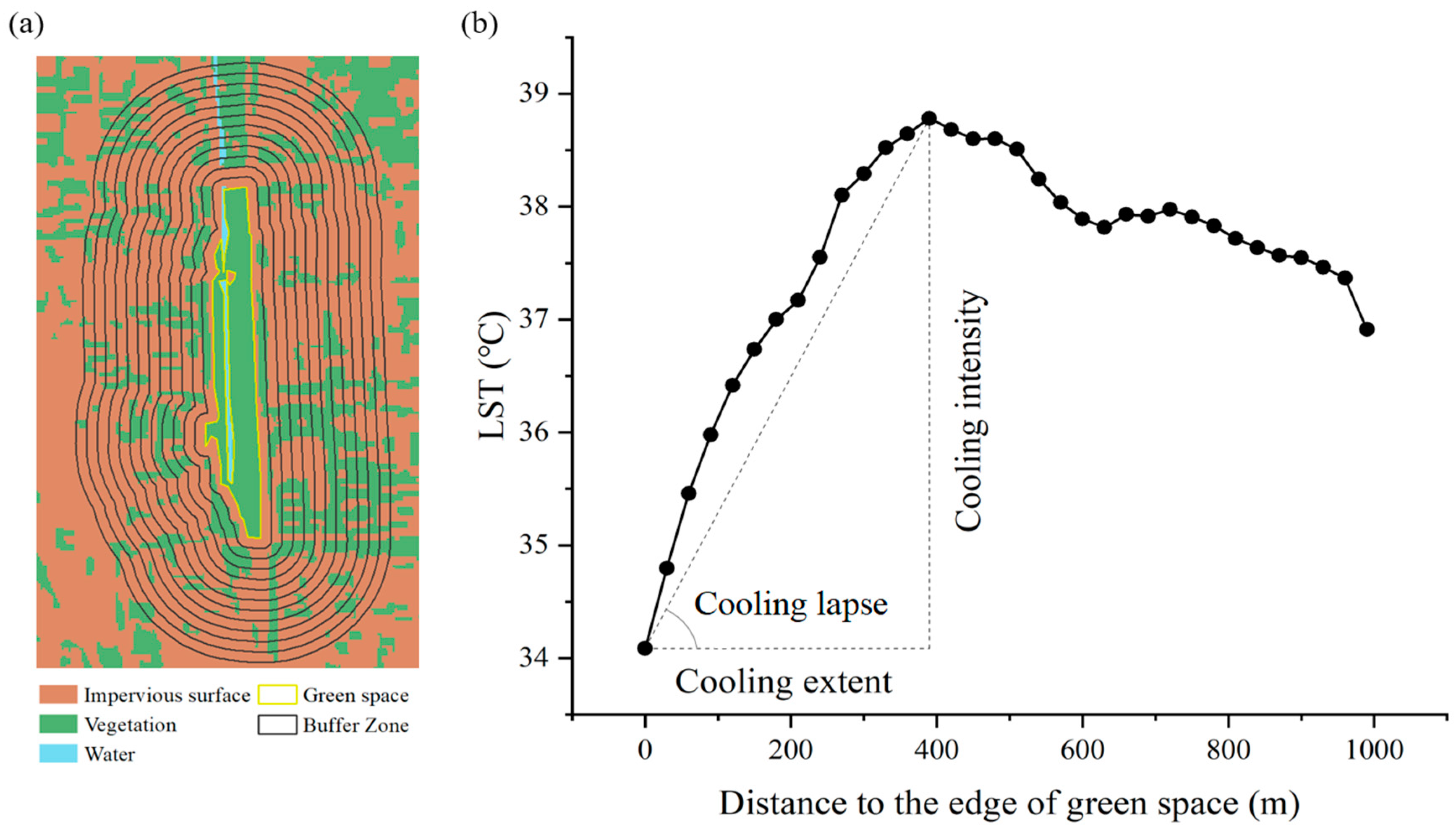
2.2. Quantification of UGSs’ Cooling Effect

UGSs’ cooling effect was quantified based on LST at 10:53 a.m. local time on 19 August 2014, retrieved from the Landsat 8 Operational Land Imager (OLI) and Thermal InfraRed Sensor (TIRS) Level-1 datasets (https://earthexplorer.usgs.gov/ accessed on 11 November 2021, Path 123, Row 32, Product ID: LC08_L1TP_123032_20140819_20170420_01_T1, with 2.5% cloud cover for the tile and zero cloud cover for study area). On this day, the maximum air temperature was 32.4 °C, the minimum air temperature was 21.3 °C, the mean air temperature was 26.6 °C, the average humidity degree was 62%, the rainfall was 0 mm, and the maximum wind speed was 4.4 m/s, suggesting that the breeze had little impact on the spatial distribution of LST (climate station ID-54511, 39°48′, 116°28′, Beijing, http://data.cma.cn/ accessed on 11 November 2021). Landsat 8 OLI bands are with a 30 m spatial resolution and the two TIRS thermal infrared bands are with a 100 m spatial resolution, which were resampled to match the resolution of OLI bands before the release of Landsat Level-1 data. Atmospheric correction was conducted via the Second Simulation of the Satellite Signal in the Solar Spectrum (6S) [30] for the acquisition of the surface reflectance of red and near infrared bands. Due to the meteorological conditions on that day (mean air temperature of 26.6 °C, cloud-free day with no rainfall), the atmospheric model of mid-latitude summer was adopted. The aerosol optical depth (AOD) was derived based on the dark-object method, with the help of blue, red, and short-wave infrared (2.1 μm) bands of Landsat data [31,32], serving as input of atmospheric correction. LST was retrieved via a practical split-window algorithm, with an accuracy better than 1.0 °C [33,34]. To be specific, LST was retrieved as:

$$\mathrm{LST}= c_0+\left(c_1+c_2\frac{1-\epsilon }{\epsilon }+c_3\frac{\Delta \epsilon }{{\epsilon }^2}\right)\frac{T_1+T_2}{2}+\left(c_4+c_5\frac{1-\epsilon }{\epsilon }+c_6\frac{\Delta \epsilon }{{\epsilon }^2}\right)\frac{T_1-T_2}{2}+c_7{\left(T_1-T_2\right)}^2$$

(2)

where $T_1$ and $T_2$ are the top of atmosphere (TOA) brightness temperatures in thermal band 1 (band 10 of Landsat 8) and in thermal band 2 (band 11 of Landsat 8), respectively; $c_0, c_1,\dots ,c_7$ refer to the coefficients derived from water vapor (wv) and the simulated dataset [33]; and ε and ∆ε are the mean value and the difference value (∆ε = ${\epsilon }_1-{\epsilon }_2$) of the emissivity in the two thermal bands. Moreover, wv was estimated as [34]:

$$wv=-9.674{\left(\frac{{\tau }_2}{{\tau }_1}\right)}^2+0.653\frac{{\tau }_2}{{\tau }_1}+9.087$$

(3)

$$\frac{{\tau }_2}{{\tau }_1}\approx \frac{{{\displaystyle \sum }}_{k=1}^N\left(T_{1,k}-\overline{T_1}\right)\left(T_{2,k}-\overline{T_2}\right)}{{{\displaystyle \sum }}_{k=1}^N{\left(T_{2,k}-\overline{T_2}\right)}^2}$$

(4)

where ${\tau }_1$ and ${\tau }_2$ are the upward atmospheric transmittances of the two thermal bands; N is the total number of pixels in the applied moving window (N = n ∗ n and n = 10 in this algorithm); $T_{1,k}$ and $T_{2,k}$ are the TOA brightness temperatures of the two thermal bands for the kth pixel; and $\overline{T_1}$ and $\overline{T_2}$ are the average TOA brightness temperatures of the two thermal bands in the given moving window. In addition, the emissivity ε was calculated as:

$$\epsilon ={\epsilon }_{v}f+{\epsilon }_g\left(1-f\right)+4\langle d\epsilon \rangle f\left(1-f\right)$$

(5)

$$f=\{\begin{array}{cc}\hfill 1,& \mathrm{NDVI}\ge {\mathrm{NDVI}}_v \hfill \\ \hfill {\left(\frac{\mathrm{NDVI}-{\mathrm{NDVI}}_s}{{\mathrm{NDVI}}_v-{\mathrm{NDVI}}_s}\right)}^2,& {\mathrm{NDVI}}_s<\mathrm{NDVI}<{\mathrm{NDVI}}_v\hfill \\ \hfill 0,& \mathrm{NDVI}\le {\mathrm{NDVI}}_s\hfill \end{array}$$

(6)

where ${\epsilon }_v$ and ${\epsilon }_g$ are the emissivity of vegetation and background, respectively, derived from the spectrum dataset; $\langle d\epsilon \rangle$ refers to the parameters of cavity effect; f is the vegetation fraction; NDVI is the normalized difference vegetation index derived from Landsat OLI bands; ${\mathrm{NDVI}}_v$ and ${\mathrm{NDVI}}_s$ are NDVI of bare soil and dense vegetation, set as 0.86 and 0.2, separately. The retrieval of LST was conducted in a software integrating the algorithms above [33].

The cooling effect of UGSs was quantified by three metrics (Figure 3): Green spaces’ cooling intensity (CI), cooling extent (CE), and cooling lapse (CL) [35]. CE (unit: m) is expressed as the maximum distance between the edge of UGS and the first turning point of the temperature curve. CI (unit: °C) is the LST difference between the green space and the first turning point. CL (unit: °C/km) is the LST drop with unit distance. These metrics have been widely used in previous relevant studies and have been proven as effective to quantify the cooling effect of green spaces [21,36,37].

2.3. Potential Factor Analysis

Both the internal and external factors were considered for each green space (Table 1). The internal factors are (1) the area, (2) the shape index characterized by the landscape shape index (LSI), and (3) the quality of vegetation indicated by the normalized difference vegetation index (NDVI) based on SPOT 6 images.

The external factors are mainly from two sources: One is from the external green patches, the other is from the adjacent water. The first kind of external factor includes: (1) Distance to the external green patches, indicated by the area-weighted mean Euclidean nearest-neighbor distance (ENN_AM), (2) quantity of external vegetation patches within CE, indicated by the percentage of vegetation area (PLAND), and (3) distribution pattern for the external green patches within CE, indicated by the mean fractal dimension index (FRAC_MN) [38]. The second kind of external factor originated from the adjacent water, including (4) distance to the nearest water patch (W_DIST) and (5) adjacent water quantity indicated by the water proximity index (W_PROX). W_PROX was calculated as: The sum of water body area within a certain distance divided by the nearest edge-to-edge distance squared between each water body and the specific green space. Earlier research suggested that the water body’s cooling extent was within 600 m in Beijing [39]. Therefore, for each green space, whether there was water within 600 m of the space was examined and W_PROX within 600 m was calculated.

The analysis of variance (ANOVA) is used to test the significant difference of UGSs among different groups such as locations within the 2nd, 3rd, and 4th ring or with a different dominant vegetation. Moreover, multivariable stepwise regressions were used to analyze the driving factors of green spaces’ thermal characteristics, with LST, CI, CE, and CL as dependent variables and the internal and external factors as independent variables. All of the variables were standardized before the regression. Furthermore, the correlation analyses were conducted between the thermal characteristics of UGS (LST, CI, CE, and CL) and the potential factors among UGSs in different area groups.

Table 1. Potential factors included in this study.

Factors	Abbreviations	Formula	Descriptions
Area of green space	Area	-	The area of each green space.
Landscape shape index	LSI	$\frac{P}{2\sqrt{\pi A}}$ [40]	A standardized measure of edge density adjusting for the size of green space and a circle standard. P and A refer to the perimeter and area of UGS, separately.
Normalized difference vegetation index	NDVI	$\frac{NIR-R}{NIR+R}$ [41]	A normalized measure of vegetation growth or its density. NIR and R refer to the UGS surface reflectance of near-infrared and red bands, separately.
Area-weighted mean Euclidean Nearest-Neighbor distance	ENN_AM	${{\displaystyle \sum }}_{i=1}^n{d}_i\frac{a_i}{{{\displaystyle \sum }}_{j=1}^n{a}_j}$ [38]	The area-weighted mean distance of every vegetation patch to its nearest vegetation patch neighbor within the cooling extent of UGS. In the formula, a and d refer to the area of vegetation patch and distance to its nearest vegetated neighbor patch, and n refers to the number of vegetation patches.
Percentage of landscape (vegetation) area	PLAND	$\frac{{{\displaystyle \sum }}_{i=1}^n{a}_i}{A}$ [38]	The area proportion of vegetation within the UGS cooling extent, with a referring to the area of single vegetation patch of n patches within the cooling extent that has an area of A.
Mean fractal dimension index	FRAC_MN	$\frac{{{\displaystyle \sum }}_{i=1}^{n}2\ln \left(0.25p_i\right)/\ln a_i}{n}$ [38]	The average fractal dimension of vegetation patches within the cooling extent of UGS, which reflects shape complexity. For vegetation patches with a number of n, patch i has a perimeter of pi and an area of ai.
Distance to the nearest water patch	W_DIST	-	The distance between the UGS and its nearest water patch.
Water proximity	W_PROX	${{\displaystyle \sum }}_{i=1}^n\frac{a_i}{d_i^2}$ [38]	Adjacent water quantity indicated by a proximity index. The area a of a water body divided by the square of distance d between the UGS and water body is a single part of water proximity. The final water proximity is the sum of every single water proximity of n water bodies within a 600-m range from a given UGS.

Table 1. Potential factors included in this study.

Factors	Abbreviations	Formula	Descriptions
Area of green space	Area	-	The area of each green space.
Landscape shape index	LSI	$\frac{P}{2\sqrt{\pi A}}$ [40]	A standardized measure of edge density adjusting for the size of green space and a circle standard. P and A refer to the perimeter and area of UGS, separately.
Normalized difference vegetation index	NDVI	$\frac{NIR-R}{NIR+R}$ [41]	A normalized measure of vegetation growth or its density. NIR and R refer to the UGS surface reflectance of near-infrared and red bands, separately.
Area-weighted mean Euclidean Nearest-Neighbor distance	ENN_AM	${{\displaystyle \sum }}_{i=1}^n{d}_i\frac{a_i}{{{\displaystyle \sum }}_{j=1}^n{a}_j}$ [38]	The area-weighted mean distance of every vegetation patch to its nearest vegetation patch neighbor within the cooling extent of UGS. In the formula, a and d refer to the area of vegetation patch and distance to its nearest vegetated neighbor patch, and n refers to the number of vegetation patches.
Percentage of landscape (vegetation) area	PLAND	$\frac{{{\displaystyle \sum }}_{i=1}^n{a}_i}{A}$ [38]	The area proportion of vegetation within the UGS cooling extent, with a referring to the area of single vegetation patch of n patches within the cooling extent that has an area of A.
Mean fractal dimension index	FRAC_MN	$\frac{{{\displaystyle \sum }}_{i=1}^{n}2\ln \left(0.25p_i\right)/\ln a_i}{n}$ [38]	The average fractal dimension of vegetation patches within the cooling extent of UGS, which reflects shape complexity. For vegetation patches with a number of n, patch i has a perimeter of pi and an area of ai.
Distance to the nearest water patch	W_DIST	-	The distance between the UGS and its nearest water patch.
Water proximity	W_PROX	${{\displaystyle \sum }}_{i=1}^n\frac{a_i}{d_i^2}$ [38]	Adjacent water quantity indicated by a proximity index. The area a of a water body divided by the square of distance d between the UGS and water body is a single part of water proximity. The final water proximity is the sum of every single water proximity of n water bodies within a 600-m range from a given UGS.

3. Results

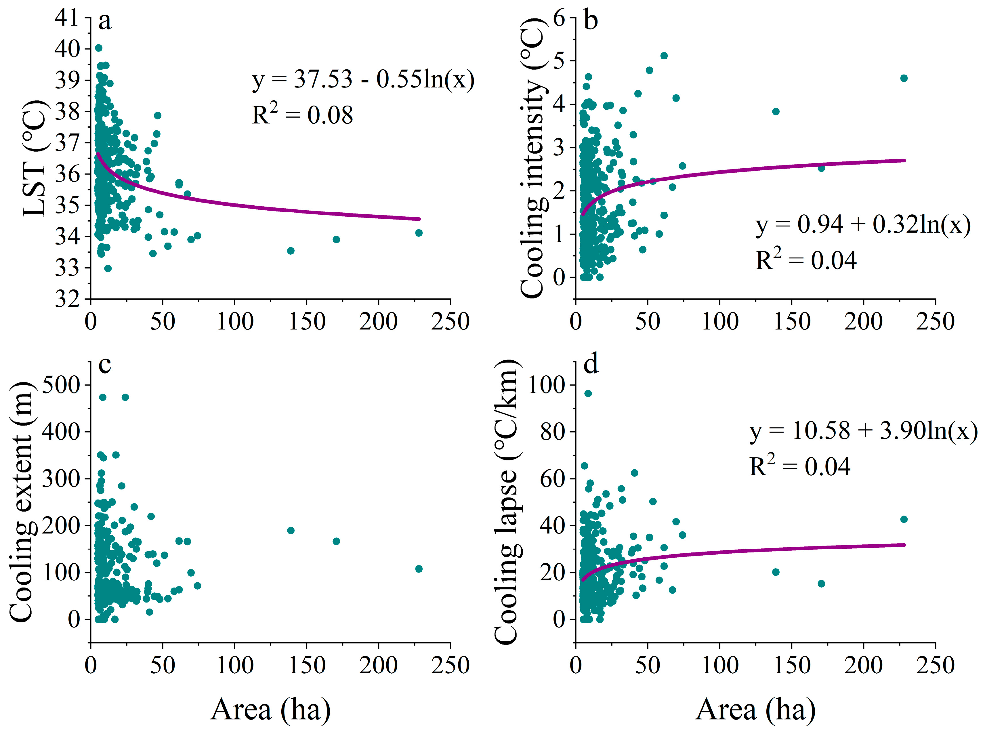
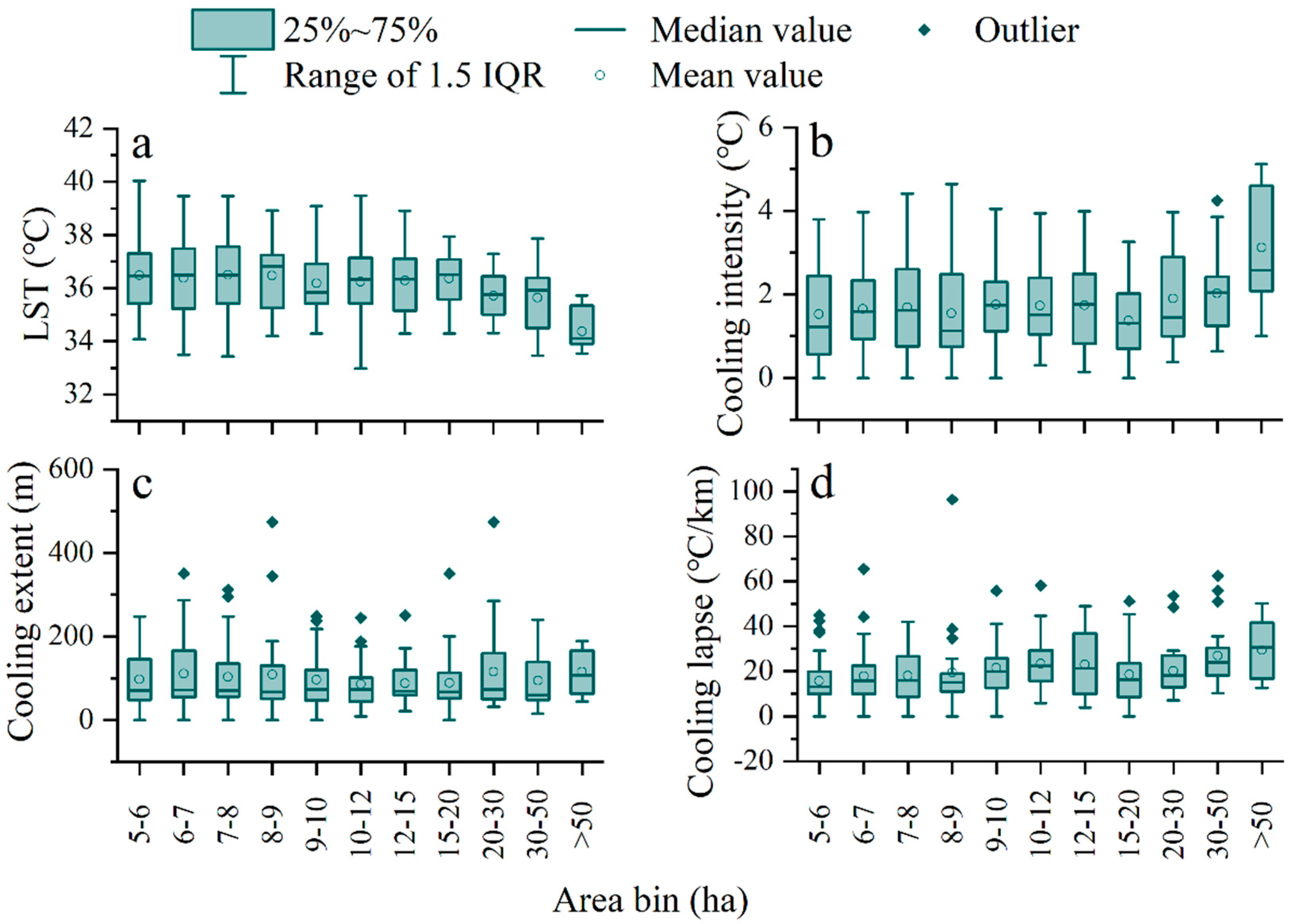
3.1. UGSs’ Cooling Effect Using Various Indicators in Beijing

The average LST of 316 UGSs was 36.2 ± 1.4 °C (Figure 4a), a 2.0 °C cooler difference than the average thermal condition of impervious surface (i.e., 38.2 °C). The minimum and maximum UGSs’ LST were 32.9 and 40.0 °C, respectively. Overall, 294 (93.0%) UGSs were with a lower LST than 38.2 °C. Three metrics of UGSs’ cooling effect were shown in Figure 3b–d: UGSs’ CE averaged at 100.0 ± 74.4 m, with a maximum value of 474.0 m; CI averaged at 1.7 ± 1.1 °C, maximized at 5.1 °C; and CL was 20.0 ± 12.9 °C/km, maximized at 96.3 °C/km. Ten UGSs lacked the cooling effect with zero CE, CI, and CL, whereas 306 (96.8%) UGSs were with a significant cooling island effect. ANOVA showed that the CE of UGSs within the 2nd ring (averaged at 132.0 m) was significantly larger than the 3rd ring (averaged at 87.3 m) and 4th ring (averaged at 98.3 m, p < 0.05). Moreover, the CI is significantly larger for UGSs within the 2nd ring (averaged at 1.97 °C) than UGSs within the 3rd ring (averaged at 1.53 °C). This indicates that UGSs closer to the city center have a better cooling effect. The urban core area with less vegetation cover and more active human activities has a higher LST, where the cooling effect of UGSs is more prominent.

With respect to dominant vegetation, ANOVA also showed that there was no significant difference among UGSs with different types of dominant vegetation (the tree-based, grass-based, and mixture green spaces) for the four cooling metrics. In this study, however, only few UGSs are not dominated by trees. This characteristic of our samples could not draw conclusions of the effect of vegetation type on the cooling effect of UGSs.

3.2. Identify the Driving Factors of UGSs’ Cooling Effect

The statistics analysis proved that the area of green spaces is negatively correlated with LST (Figure 5a, p < 0.01), positively correlated with CI (Figure 5b, p < 0.01), and CL (Figure 5d, p < 0.01). Although larger green spaces were with a lower LST, higher CI, and larger CL, the area is not a determining factor of UGSs’ cooling effect. Green spaces with a large area (>50 ha) generally have a good performance on cooling. Small area green spaces (<50 ha) have a larger range of the four cooling indicators, suggesting the large potential for urban warming mitigation.

The result of multiple regression shows that the four cooling indicators are all highly significantly correlated with NDVI (p < 0.001), and NDVI is the primary driver for all of the four indicators (

Table 2. Standardized regression coefficient in the multiple linear regression results with LST, CI, CE, and CL as dependent variables and the internal and external factors as independent variables (Note: NDVI and LSI are internal factors; ENN_AM (area-weighted mean Euclidean nearest-neighbor distance to external vegetation patches), PLAND (percentage of landscape occupied by external vegetation patches), FRAC_MN (mean fractal dimension index), and W_DIST (distance to the nearest water patch)). The internal and external factors that are not significant among all of the four dependent variables are not shown in this table.

Cooling Effect	Internal Factors		External Factors				Adj-R2
	NDVI	LSI	ENN_AM	PLAND	FRAC_MN	W_DIST
LST	−0.561					0.208	0.40
Cooling intensity	0.470	−0.206		−0.408			0.35
Cooling extent	0.138	−0.150			−0.191		0.07
Cooling lapse	0.369		0.202				0.17

). NDVI and W_DIST are the first two primary drivers for LST variation (Adj-R² = 0.40). The increase in the water body nearby could lead to a lower LST inside the green space. The CI is negatively correlated with PLAND and LSI (p < 0.001), which indicates that the less complicated shape of the green spaces and lower PLAND of the external vegetation patches lead to a greater CI. NDVI, PLAND, and LSI explain 35% of the variation of CI. In addition to NDVI, CE is highly significantly correlated with FRAC_MN and LSI at the 0.001 level, showing that a less complicated shape of the green spaces or outside the green spaces leads to a greater CE. NDVI, FRAC_MN, and LSI explain the little variation (7%) of CE. In addition to NDVI, the area-weighted mean Euclidean nearest-neighbor distance to external vegetation patches (ENN_AM) is the primary driver for CL, showing a positive correlation with CL (p < 0.001).

3.3. Maximize the Cooling Performance of UGSs within the Limited Green Space Area

UGSs were grouped into 11 levels according to their area bins (5–6, 6–7, 7–8, 8–9, 9–10, 10–12, 12–15, 15–20, 20–30, 30–50, and >50, in unit of ha, Figure 6). Despite the difference in the UGS area, no significant difference is shown among the different area bins except for UGS, which is larger than 50 ha. UGSs in the same area bins could own a LST variability of ~6 °C. UGSs’ cooling effect shows a large variance for each area bin, which indicates the potential (the optimization for each bin) of the cooling effect when the area of UGS is restricted.

The variation of UGSs’ cooling effect is strongly correlated with NDVI, LSI, and landscape structure. However, the significance of the relationship changed greatly with the area bins and the specific indicators (Figure 7). Generally, LSI and NDVI are significantly correlated with LST. In addition, the three cooling effect metrics reached the greatest correlation at area 8–9 ha. As for the external factors, PLAND and FRAC_MN are negatively correlated with LST at area 8–9 ha, indicating that the increasing quantity and fragmented distribution of vegetation around the green space promote cooler green spaces. Moreover, LST is positively correlated with W_DIST and negatively correlated with W_PROX, in particular, at area bins ranging from 6–20 ha. In these area bins, UGSs with the cooler LST are often near water, whereas the hottest UGSs are far from water and with a lower water proximity. CI and CL are positively correlated with ENN_AM and negatively correlated with PLAND, in particular, at area 5–7 ha and 12–20 ha, which indicate that the increasing quantity and closer external vegetation would hide UGSs’ cooling intensity and lapse. Meanwhile, FRAC_MN is positively correlated with CL at area 12–30 ha, suggesting that the fragmented external vegetation would increase CL more than the aggregated ones. CE is positively correlated with ENN_AM in specific bins of 5–6 ha and 20–30 ha, indicating that the distance to the nearest-neighboring patch of green space would influence the turning point of temperature curve.

4. Discussion

4.1. The Cooling Effect of UGSs in the Metacity Beijing

Of the 316 UGSs (96.8%), 306 have a significant cooling island effect. The average LST of 316 green spaces is 36.2 ± 1.4 °C, with a cooling extent of 100.0 ± 74.4 m, 1.7 ± 1.1 °C cooling intensity, and a resultant 20.0 ± 12.9 °C/km cooling lapse. Lin et al. [42] reported that CI ranges from 2.3 to 4.8 °C and CE ranges from 85–284 m in Beijing. Naeem et al. [26] found an average cooling intensity of 2.98 °C among 22 green space samples in Beijing. The slight difference in magnitude might be due to the difference in the selected UGSs. Generally, UGSs in metacities have shown a stronger cooling effect. As for the other metacity (Shanghai) in China, Du et al. [21] found CI of 3.0 °C and CE of 570 m on average in UGSs of Shanghai. Comparably, UGSs in cities with a population less than 20 million have CI less than 2 °C, such as 1.78 °C in Fuzhou, China [23], 1.6 °C in Milan, Italy [43], and 1.3 °C in Nagoya, Japan [44]. On the other hand, the maximum CI in metacities is not necessarily greater than in the smaller cities. UGSs in Beijing have a maximum CI of 5.1 °C, whereas those in Nagoya have a maximum CI of 6.8 °C [44]. Denser human activities and a higher LST result in a greater average CI in metacities in general, while the maximum CI, which is more dependent on the block-scale condition, can reach a higher level regardless of the city scale.

Most of the earlier studies selected a very limited number of UGSs with a relatively large area. For example, Peng et al. [22] only selected 24 UGSs larger than 600 ha in Shenzhen, China, whereas this study chose 316 UGSs with a variety of areas in Beijing. The UGSs in this study included many small and irregular-shaped ones, which would lower the average CI and CE in Beijing. The UGSs area and rank fit the Pareto distribution (with 0.71 Pareto coefficient and R² = 0.98), indicating that mass UGSs are small, whereas large UGSs are rare. Green spaces with a larger area usually have a better ability to mitigate that heat effect, as there is more vegetation inside the green space and NDVI is larger. However, as urbanization is nearly an irreversible progress around our globe, the vegetated area in the urban environment is limited and cannot be enlarged easily. It is impractical to mitigate the urban heat problem and heat wave effect by only enlarging the green space. Small and dispersive green spaces are rarely discussed. However, they spread all over the metacities, many of whom are distributed inside or between blocks, and are therefore, more accessible for urban residents and closely linked to the well-being of numerous citizens. Regardless of the area, green spaces can maintain a ~6 °C LST difference and a ~5 °C CI difference between the best and the worst situations (Figure 6a,b). Green spaces with small sizes have a great potential to reach the best cooling situation.

4.2. Landscape Structure Drivers of UGSs’ Cooling Effect

For the four cooling indicators of UGSs, LST indicates thermal condition under certain green space context, whereas the other three particularly emphasize the cooling effect of the surroundings. For the internal factors, NDVI has significant coefficients with LST and the other cooling effect indicators. The higher NDVI corresponding to a denser vegetation, leads to a lower LST in UGSs, due to the evapotranspiration process of vegetation, and consequently, the stronger cooling effect (CI, CE, and CL). Vegetation density plays a significant role in both cooling the UGS itself and cooling the surroundings. As for LSI, which suggests the edge complexity of vegetation patch, the UGS with a higher LSI has a more complex edge. This promotes the heat exchange between the UGS and the surrounding environment and results in a higher LST, and thus, lower CI. Du et al. [21] found that a high LSI will improve the cooling intensity of green spaces, but the selected green spaces were limited by numbers, leading to a result that all of the LSI values are lower than 4. In this study, there are more than 200 green spaces with an LSI value higher than 4. Different LSI ranges may lead to different conclusions. There might be a trade-off between keeping the cooler temperature inside the green space and cooling down the surroundings through the heat exchange.

In addition, the surrounding vegetation and water influence UGSs’ cooling effect. The water body (W_DIST and W_PROX) shows a strong effect only on LST (Figure 7a), suggesting that the water body nearby is helpful for the reduction of LST for UGSs. This is due to the fact that the water body has a higher heat capacity and a stronger effect of evaporation than vegetation or impervious surface, which results in a great heat storage in the daytime and causes considerable cooling effects. Moreover, it can be found that the water body has a more significant effect on LST than on the three cooling effect metrics. On the one hand, this may be due to the fact that the water body cools itself and the surroundings. On the other hand, it weakens part of the independence of the cooling effects of the adjacent green space.

As for the metrics reflecting the surrounding vegetation, PLAND mainly shows a negative correlation with CI, CE, and CL, indicating that more surrounding vegetation might veil the cooling effect of UGS to the surroundings. The positive correlation between ENN_AM and CI indicates that more vegetation in a close spatial range weakens CI by decreasing the temperature difference between UGSs and the surroundings. The correlation between CL and FRAC_MN is significantly negative for 6–7 ha UGSs, but it turns positive for 12–30 ha UGSs. FRAC_MN reveals the average shape complexity of the surrounding vegetation, which is similar to LSI in that it has a positive correlation with LST. The correlation between CL and FRAC_MN may suggest that when the shape of the surrounding vegetation is more regular, which indicates a lower LST in the surrounding vegetation, a UGS with at least 12 ha can integrate the cooling effect of itself and the surrounding vegetation to make a much gentle cooling lapse with a longer cooling extent (considering the negative correlation between CE and FRAC_MN for UGSs of 12–30 ha).

Generally, it can be found that the internal factors (NDVI and LSI) have stronger effects on UGSs’ cooling effect than the external factors, which suggest that the quality of the green space may be more important than the surrounding landscape configuration with regards to UGSs’ cooling effect. Moreover, it is shown that CE is less likely to be influenced by the potential factors and remained relatively stable among the area groups (Figure 6 and Figure 7). Furthermore, previous studies found cooling extents of ~100 m, with a maximum CE of no more than 300 m [23,42,45]. This may be due to the fact that the complicated 3D structure in the urban area blocks the flow of heat and disturbs the detection of LST.

4.3. Implications for Urban Planning and Climate Mitigation

This study may provide practical strategies for the maximization of the cooling performance of UGSs for different purposes in urban heating mitigation. Generally, vegetation density, represented by NDVI, is a key factor for UGSs’ cooling effects. Green spaces with a denser vegetation have a greater cooling effect, which is consistent with the previous studies [45,46]. A denser vegetation not only prevents the land surface from being heated directly, but also increases the amount of evapotranspiration cooling. A larger size of green space would benefit from a better cooling effect, i.e., lower LST, higher CI, and larger CL. However, when the size is limited, which is a usual scene in metacities, a regular and compact shape would lead to lower LST and higher CI efficiently, which provide a cooling service for the UGSs users directly. Moreover, similar results are found in other cities, e.g., Nagoya in Japan, Nanjing and Fuzhou in China [44,47,48]. Our study suggests that an UGS, which is more compact in shape and vegetation indicating a less complicated boundary and denser vegetation, has a better cooling effect. Many earlier researches have quantified the threshold size for the best size of blue-green space to achieve the best cooling effect [24]. Using 316 UGSs in Beijing, China, this study found that UGSs with the same area bin varied in providing the cooling service. This indicates that the present UGSs have a large cooling potential without enlarging their area, which is essential for actionable planning to alleviate the urban heating climate.

Moreover, this study explored the external factors of UGSs, which have their influences on the cooling effects under certain conditions. Specifically, when designing a green space with a lower LST, it is best to introduce the water nearby to couple the green and blue space together for tourists and residents. Furthermore, it is shown that small UGSs (<8 ha) could be influenced easily by the external vegetation PLAND. In order to release the potential of CI and CL, UGSs with an area smaller than 8 ha should be first placed in areas with little vegetation cover. The farther distance to the external vegetation helps in the enlargement of CE and acceleration of CL. For UGSs with an area of 12~30 ha, UGSs can create a more effective CL, considering FRAC_MN with irregular vegetation patches around. Our findings may be helpful for urban planners of different area customized cooling services of UGSs, in order to mitigate both the urban heat island and global climate warming.

4.4. Limitations and Suggestions

This study has several limitations. There is no universal standard to define the urban green space. While some earlier studies define green spaces artificially using regular and large patches with water or pavements, this study defines green spaces as all of the vegetated patches greater than 5 ha. Of note, much smaller UGSs (<5 ha) such as street trees and pocket parks also have an important cooling effect. Therefore, more attention should be paid to urban small UGSs in further studies. Meanwhile, SPOT 6 data provide finer spatial details than Landsat data with a 30 m resolution. The finer resolution remote sensing data allow us to discover more details of the UGSs inside the blocks. Compared to the method of selecting relatively large green spaces [21,22], which ensure green space completeness in the human-defined area, the method of this study pays more attention to the spatial location and distribution of vegetated pixels that are adjacent or nearby, regardless of whether they correspond to human-defined boundaries. Other possible factors that may affect the green spaces’ cooling effect, such as vegetation species, UGSs’ irrigation, urban morphology, and 3D structure of buildings, are worth studying in future studies [13,49]. As for LST, the derived LST has a rough spatial resolution, which is sourced from the TIR sensor. In addition, the LST derived through remote sensing still has large disparities with the air temperature. Air temperature not only reflects the heat exchange between UGSs and the surroundings directly, but also influences the residents’ outdoor thermal comfort [50]. Future researches combining both the surface and air temperature are needed to elucidate the mechanisms of UGSs’ cooling effect. Additionally, the elevation factor was not taken into consideration, since the urban core area of Beijing enjoys a flat terrain. Nonetheless, it should be included in the analysis when evaluating the cooling effect of the green spaces in other metacities with a hilly topography, since elevation is an important factor that influences LST.

5. Conclusions

One of the greatest benefits from UGSs is the cooling effect, which helps mitigate the urban heating climate. The impact of 316 UGSs on the urban thermal environment in Beijing is quantified as four metrics: LST, CI, CE, and CL with SPOT 6 and Landsat images. The average LST of 316 green spaces, which is larger than 5 ha, is 36.2 ± 1.4 °C, with a cooling extent of 100.0 ± 74.4 m, 1.7 ± 1.1 °C cooling intensity, and a resultant 20.0 ± 12.9 °C/km cooling lapse. UGSs surrounded by areas with denser human activities and a higher LST are with a higher CI. The multiple regression result shows that LST, CI, CE, and CL are significantly correlated to NDVI. In addition, CI and CE are negatively significantly correlated to LSI, while external landscape factors have various influences on LST and the cooling effects. Furthermore, UGSs smaller than 9 ha own a LST variability of ~6 °C, suggesting the great potential of cooling effects from these UGSs. The correlation analysis among the same area bins of UGSs confirms the key role of NDVI and LSI, while external factors have a significant correlation with the cooling effects in specific area bins. CE is less likely to be affected by the landscape structure. To provide advice on urban planning, it is clear that UGSs that are compact in shape or with a denser vegetation, have a better cooling effect. As for the external factors, the water body nearby could be introduced to couple the green and blue space for better cooling and thermal comfort. As human health and well-being are threatened by severe urban heating, our finding may provide solutions for the mitigation of both the urban heat island and global climate warming of the UGS area customized cooling service.

References

1. Mullaney, J.; Lucke, T.; Trueman, S.J. A Review of Benefits and Challenges in Growing Street Trees in Paved Urban Environments. Landsc. Urban Plan. 2015, 134, 157–166. [Google Scholar] [CrossRef]
2. Chen, M.; Dai, F.; Yang, B.; Zhu, S. Effects of Neighborhood Green Space on PM2.5 Mitigation: Evidence from Five Megacities in China. Build. Environ. 2019, 156, 33–45. [Google Scholar] [CrossRef]
3. Wouters, H.; Ridder, K.D.; Demuzere, M.; Lauwaet, D.; Van Lipzig, N.P.M. The Diurnal Evolution of the Urban Heat Island of Paris: A Model-Based Case Study during Summer 2006. Atmos. Chem. Phys. 2013, 13, 8525–8541. [Google Scholar] [CrossRef] [Green Version]
4. Weissert, L.F.; Salmond, J.A.; Schwendenmann, L. A Review of the Current Progress in Quantifying the Potential of Urban Forests to Mitigate Urban CO2 Emissions. Urban Clim. 2014, 8, 100–125. [Google Scholar] [CrossRef]
5. Beninde, J.; Veith, M.; Hochkirch, A. Biodiversity in Cities Needs Space: A Meta-Analysis of Factors Determining Intra-Urban Biodiversity Variation. Ecol. Lett. 2015, 18, 581–592. [Google Scholar] [CrossRef] [PubMed]
6. Jennings, V.; Larson, L.; Yun, J. Advancing Sustainability through Urban Green Space: Cultural Ecosystem Services, Equity, and Social Determinants of Health. Int. J. Environ. Res. Public Health 2016, 13, 196. [Google Scholar] [CrossRef] [Green Version]
7. Jia, W.; Zhao, S. Trends and Drivers of Land Surface Temperature along the Urban-Rural Gradients in the Largest Urban Agglomeration of China. Sci. Total Environ. 2020, 711, 134579. [Google Scholar] [CrossRef]
8. Ward, K.; Lauf, S.; Kleinschmit, B.; Endlicher, W. Heat Waves and Urban Heat Islands in Europe: A Review of Relevant Drivers. Sci. Total Environ. 2016, 569–570, 527–539. [Google Scholar] [CrossRef]
9. Zhou, D.; Zhao, S.; Zhang, L.; Sun, G.; Liu, Y. The Footprint of Urban Heat Island Effect in China. Sci. Rep. 2015, 5, 11160. [Google Scholar] [CrossRef] [PubMed]
10. United Nations Department for Economic and Social Affairs. World Urbanization Prospects 2018; United Nations Department for Economic and Social Affairs: New York, NY, USA, 2018. [Google Scholar]
11. Peng, J.; Xie, P.; Liu, Y.; Ma, J. Urban Thermal Environment Dynamics and Associated Landscape Pattern Factors: A Case Study in the Beijing Metropolitan Region. Remote Sens. Environ. 2016, 173, 145–155. [Google Scholar] [CrossRef]
12. Su, Y.; Liu, L.; Liao, J.; Wu, J.; Ciais, P.; Liao, J.; He, X.; Liu, X.; Chen, X.; Yuan, W. Phenology Acts as a Primary Control of Urban Vegetation Cooling and Warming: A Synthetic Analysis of Global Site Observations. Agric. For. Meteorol. 2020, 280, 107765. [Google Scholar] [CrossRef]
13. Doick, K.J.; Peace, A.; Hutchings, T.R. The Role of One Large Greenspace in Mitigating London’s Nocturnal Urban Heat Island. Sci. Total Environ. 2014, 493, 662–671. [Google Scholar] [CrossRef] [PubMed]
14. Hamada, S.; Ohta, T. Seasonal Variations in the Cooling Effect of Urban Green Areas on Surrounding Urban Areas. Urban For. Urban Green. 2010, 9, 15–24. [Google Scholar] [CrossRef]
15. Oliveira, S.; Andrade, H.; Vaz, T. The Cooling Effect of Green Spaces as a Contribution to the Mitigation of Urban Heat: A Case Study in Lisbon. Build. Environ. 2011, 46, 2186–2194. [Google Scholar] [CrossRef]
16. Ziter, C.D.; Pedersen, E.J.; Kucharik, C.J.; Turner, M.G. Scale-Dependent Interactions between Tree Canopy Cover and Impervious Surfaces Reduce Daytime Urban Heat during Summer. Proc. Natl. Acad. Sci. USA 2019, 116, 7575–7580. [Google Scholar] [CrossRef] [Green Version]
17. Qiu, K.; Jia, B. The Roles of Landscape Both inside the Park and the Surroundings in Park Cooling Effect. Sustain. Cities Soc. 2020, 52, 101864. [Google Scholar] [CrossRef]
18. Wang, J.; Zhou, W.; Jiao, M.; Zheng, Z.; Ren, T.; Zhang, Q. Significant Effects of Ecological Context on Urban Trees’ Cooling Efficiency. ISPRS J. Photogramm. Remote Sens. 2020, 159, 78–89. [Google Scholar] [CrossRef]
19. Yao, L.; Li, T.; Xu, M.; Xu, Y. How the Landscape Features of Urban Green Space Impact Seasonal Land Surface Temperatures at a City-Block-Scale: An Urban Heat Island Study in Beijing, China. Urban For. Urban Green. 2020, 52, 126704. [Google Scholar] [CrossRef]
20. Liao, W.; Cai, Z.; Feng, Y.; Gan, D.; Li, X. A Simple and Easy Method to Quantify the Cool Island Intensity of Urban Greenspace. Urban For. Urban Green. 2021, 62, 127173. [Google Scholar] [CrossRef]
21. Du, H.; Cai, W.; Xu, Y.; Wang, Z.; Wang, Y.; Cai, Y. Quantifying the Cool Island Effects of Urban Green Spaces Using Remote Sensing Data. Urban For. Urban Green. 2017, 27, 24–31. [Google Scholar] [CrossRef]
22. Peng, J.; Dan, Y.; Qiao, R.; Liu, Y.; Dong, J.; Wu, J. How to Quantify the Cooling Effect of Urban Parks? Linking Maximum and Accumulation Perspectives. Remote Sens. Environ. 2021, 252, 112135. [Google Scholar] [CrossRef]
23. Yu, Z.; Guo, X.; Zeng, Y.; Koga, M.; Vejre, H. Variations in Land Surface Temperature and Cooling Efficiency of Green Space in Rapid Urbanization: The Case of Fuzhou City, China. Urban For. Urban Green. 2018, 29, 113–121. [Google Scholar] [CrossRef]
24. Yu, Z.; Yang, G.; Zuo, S.; Jørgensen, G.; Koga, M.; Vejre, H. Critical Review on the Cooling Effect of Urban Blue-Green Space: A Threshold-Size Perspective. Urban For. Urban Green. 2020, 49, 126630. [Google Scholar] [CrossRef]
25. Zhou, W.; Shen, X.; Cao, F.; Sun, Y. Effects of Area and Shape of Greenspace on Urban Cooling in Nanjing, China. J. Urban Plan. Dev. 2019, 145, 04019016. [Google Scholar] [CrossRef]
26. Naeem, S.; Cao, C.; Qazi, W.; Zamani, M.; Wei, C.; Acharya, B.; Rehman, A. Studying the Association between Green Space Characteristics and Land Surface Temperature for Sustainable Urban Environments: An Analysis of Beijing and Islamabad. ISPRS Int. J. Geo-Inf. 2018, 7, 38. [Google Scholar] [CrossRef] [Green Version]
27. Beijing Municipal Bureau of Statistics. Available online: http://tjj.beijing.gov.cn/ (accessed on 5 October 2021).
28. Meng, Q.; Zhang, L.; Sun, Z.; Meng, F.; Wang, L.; Sun, Y. Characterizing Spatial and Temporal Trends of Surface Urban Heat Island Effect in an Urban Main Built-up Area: A 12-Year Case Study in Beijing, China. Remote Sens. Environ. 2018, 204, 826–837. [Google Scholar] [CrossRef]
29. Taylor, L.; Hochuli, D.F. Defining Greenspace: Multiple Uses across Multiple Disciplines. Landsc. Urban Plan. 2017, 158, 25–38. [Google Scholar] [CrossRef] [Green Version]
30. Vermote, E.F.; Tanré, D.; Deuze, J.L.; Herman, M.; Morcette, J.-J. Second Simulation of the Satellite Signal in the Solar Spectrum, 6S: An Overview. IEEE Trans. Geosci. Remote Sens. 1997, 35, 675–686. [Google Scholar] [CrossRef] [Green Version]
31. Kaufman, Y.J.; Tanré, D.; Remer, L.A.; Vermote, E.F.; Chu, A.; Holben, B.N. Operational Remote Sensing of Tropospheric Aerosol over Land from EOS Moderate Resolution Imaging Spectroradiometer. J. Geophys. Res. Atmos. 1997, 102, 17051–17067. [Google Scholar] [CrossRef]
32. Ångström, A. The Parameters of Atmospheric Turbidity. Tellus 1964, 16, 64–75. [Google Scholar] [CrossRef] [Green Version]
33. Du, C.; Ren, H.; Qin, Q.; Meng, J.; Zhao, S. A Practical Split-Window Algorithm for Estimating Land Surface Temperature from Landsat 8 Data. Remote Sens. 2015, 7, 647–665. [Google Scholar] [CrossRef] [Green Version]
34. Ren, H.; Du, C.; Liu, R.; Qin, Q.; Yan, G.; Li, Z.-L.; Meng, J. Atmospheric Water Vapor Retrieval from Landsat 8 Thermal Infrared Images. J. Geophys. Res. Atmos. 2015, 120, 1723–1738. [Google Scholar] [CrossRef]
35. Du, H.; Song, X.; Jiang, H.; Kan, Z.; Wang, Z.; Cai, Y. Research on the Cooling Island Effects of Water Body: A Case Study of Shanghai, China. Ecol. Indic. 2016, 67, 31–38. [Google Scholar] [CrossRef]
36. Yu, Z.; Xu, S.; Zhang, Y.; Jørgensen, G.; Vejre, H. Strong Contributions of Local Background Climate to the Cooling Effect of Urban Green Vegetation. Sci. Rep. 2018, 8, 6798. [Google Scholar] [CrossRef]
37. Fan, H.; Yu, Z.; Yang, G.; Liu, T.Y.; Liu, T.Y.; Hung, C.H.; Vejre, H. How to Cool Hot-Humid (Asian) Cities with Urban Trees? An Optimal Landscape Size Perspective. Agric. For. Meteorol. 2019, 265, 338–348. [Google Scholar] [CrossRef]
38. McGarigal, K. FRAGSTATS Help; University of Massachusetts: Amherst, MA, USA, 2015; p. 182. [Google Scholar]
39. Yu, K.; Chen, Y.; Liang, L.; Gong, A.; Li, J. Quantitative Analysis of the Interannual Variation in the Seasonal Water Cooling Island (WCI) Effect for Urban Areas. Sci. Total Environ. 2020, 727, 138750. [Google Scholar] [CrossRef]
40. Patton, D.R. A Diversity Index for Quantifying Habitat “Edge”. Wildl. Soc. Bull. (1973–2006) 1975, 3, 171–173. [Google Scholar]
41. Rouse, J.W. Monitoring the Vernal Advancement of Retrogradation of Natural Vegetation; Type III, Final Report; NASA/GSFC: Greenbelt, MD, USA, 1974; Volume 371. [Google Scholar]
42. Lin, W.; Yu, T.; Chang, X.; Wu, W.; Zhang, Y. Calculating Cooling Extents of Green Parks Using Remote Sensing: Method and Test. Landsc. Urban Plan. 2015, 134, 66–75. [Google Scholar] [CrossRef]
43. Mariani, L.; Parisi, S.G.; Cola, G.; Lafortezza, R.; Colangelo, G.; Sanesi, G. Climatological Analysis of the Mitigating Effect of Vegetation on the Urban Heat Island of Milan, Italy. Sci. Total Environ. 2016, 569–570, 762–773. [Google Scholar] [CrossRef]
44. Cao, X.; Onishi, A.; Chen, J.; Imura, H. Quantifying the Cool Island Intensity of Urban Parks Using ASTER and IKONOS Data. Landsc. Urban Plan. 2010, 96, 224–231. [Google Scholar] [CrossRef]
45. Feyisa, G.L.; Dons, K.; Meilby, H. Efficiency of Parks in Mitigating Urban Heat Island Effect: An Example from Addis Ababa. Landsc. Urban Plan. 2014, 123, 87–95. [Google Scholar] [CrossRef]
46. Zhou, W.; Huang, G.; Cadenasso, M.L. Does Spatial Configuration Matter? Understanding the Effects of Land Cover Pattern on Land Surface Temperature in Urban Landscapes. Landsc. Urban Plan. 2011, 102, 54–63. [Google Scholar] [CrossRef]
47. Kong, F.; Yin, H.; James, P.; Hutyra, L.R.; He, H.S. Effects of Spatial Pattern of Greenspace on Urban Cooling in a Large Metropolitan Area of Eastern China. Landsc. Urban Plan. 2014, 128, 35–47. [Google Scholar] [CrossRef]
48. Yu, Z.; Guo, X.; Jørgensen, G.; Vejre, H. How Can Urban Green Spaces Be Planned for Climate Adaptation in Subtropical Cities? Ecol. Indic. 2017, 82, 152–162. [Google Scholar] [CrossRef]
49. Li, X.; Yang, B.; Xu, G.; Liang, F.; Jiang, T.; Dong, Z. Exploring the Impact of 2D/3D Building Morphology on the Land Surface Temperature: A Case Study of Three Megacities in China. IEEE J. Sel. Top. Appl. Earth Obs. Remote Sens. 2021, 14, 4933–4945. [Google Scholar] [CrossRef]
50. Zhang, J.; Gou, Z. Tree Crowns and Their Associated Summertime Microclimatic Adjustment and Thermal Comfort Improvement in Urban Parks in a Subtropical City of China. Urban For. Urban Green. 2021, 59, 126912. [Google Scholar] [CrossRef]
Figure 1. Methodology flowchart.
Remotesensing 13 04601 g001
Figure 2. (a) Location of the study area depicted by the 4th ring road of Beijing, (b) green spaces’ distribution, and (c) the land cover. The ring road from inner to outside is the 2nd, 3rd, and 4th ring road.
Remotesensing 13 04601 g002
Figure 3. The sketch map of cooling metrics (cooling intensity, cooling extent, and cooling lapse): (a) The buffer zones around a given urban green space, and (b) the temperature curve, where the average LSTs were extracted from each 30-m buffer.
Remotesensing 13 04601 g003
Figure 4. Spatial distribution of UGS’ four cooling metrics: (a) LST, (b) cooling intensity, (c) cooling extent, and (d) cooling lapse for Beijing’s core urbanized area on 19 August 2014.
Remotesensing 13 04601 g004
Figure 5. The varying patterns of 316 urban green spaces’ four cooling metrics along their sizes for Beijing on 19 August 2014: (a) LST, (b) cooling intensity, (c) cooling extent, and (d) cooling lapse. Each green point represents one individual green space. Purple lines are logarithmic regression curves with p < 0.05.
Remotesensing 13 04601 g005
Figure 6. Box plot of urban green spaces’ four cooling metrics’ among the different area bins for Beijing on 19 August 2014: (a) LST, (b) cooling intensity, (c) cooling extent, and (d) cooling lapse.
Remotesensing 13 04601 g006
Figure 7. The Pearson correlation coefficients between green spaces’ LST and influencing factors for each area bin, among the different area bins for Beijing on 19 August 2014: (a) LST, (b) cooling intensity, (c) cooling extent, and (d) cooling lapse. *, **, and *** represent significance at the 0.05, 0.01, and 0.001 level.
Remotesensing 13 04601 g007