Article

Remote Sensing Imagery Segmentation: A Hybrid Approach

1
Faculty of Engineering and Information Technolgy, School of Computer Science, University of Technology Sydney, Sydney 2007, Australia
2
Department of Computer Science Engineering and IT, Jaypee Institute of Information Technology, Noida 201309, India
3
Department of Computer Science, Aligarh Muslim University, Aligarh 202001, India
4
Department of Mathematics, South Asian University, New Delhi 110021, India
5
Department of Computer Science and IT, Guru Ghashidash University, Bilashpur 495009, India
6
Design and Technology Vertical, Torrens University, Sydney 2007, Australia
7
Department of Electrical and Computer Engineering, University of Alberta, Edmonton, AB T6G2R3, Canada
*
Author to whom correspondence should be addressed.
Remote Sens. 2021, 13(22), 4604; https://doi.org/10.3390/rs13224604
Submission received: 26 September 2021 / Revised: 9 November 2021 / Accepted: 11 November 2021 / Published: 16 November 2021
(This article belongs to the Special Issue Remote Sensing and IoT for Smart Learning Environments)

Abstract

:
In remote sensing imagery, segmentation techniques fail to encounter multiple regions of interest due to challenges such as dense features, low illumination, uncertainties, and noise. Consequently, exploiting vast and redundant information makes segmentation a difficult task. Existing multilevel thresholding techniques achieve low segmentation accuracy with high temporal difficulty due to the absence of spatial information. To mitigate this issue, this paper presents a new Rényi’s entropy and modified cuckoo search-based robust automatic multi-thresholding algorithm for remote sensing image analysis. In the proposed method, the modified cuckoo search algorithm is combined with Rényi’s entropy thresholding criteria to determine optimal thresholds. In the modified cuckoo search algorithm, the Lévy flight step size was modified to improve the convergence rate. An experimental analysis was conducted to validate the proposed method, both qualitatively and quantitatively against existing metaheuristic-based thresholding methods. To do this, the performance of the proposed method was intensively examined on high-dimensional remote sensing imageries. Moreover, numerical parameter analysis is presented to compare the segmented results against the gray-level co-occurrence matrix, Otsu energy curve, minimum cross entropy, and Rényi’s entropy-based thresholding. Experiments demonstrated that the proposed approach is effective and successful in attaining accurate segmentation with low time complexity.

1. Introduction

Image segmentation comprises the partitioning of an image into homogenous and non-overlapping regions based on the similarity among image features such as color, intensity value, and regional statistics. Generally, it is a pre-processing step in pattern recognition and computer vision problems such as object detection, biomedical imaging, traffic control system, classification, and video surveillance. On the basis of the principle of segmentation, we built a taxonomy of various segmentation techniques that differentiates segmentation techniques based on region, edge, and thresholding.

1.1. Background

Considering the existing segmentation techniques discussed in the literature review by Sezgin and Sankur [1], the histogram-based thresholding segmentation technique holds a prime position in terms of simplicity, accuracy, and robustness. Furthermore, entropy-based approaches for thresholding are extremely popular in research due to their solid theoretical foundation in physics. Thus, entropy-based thresholding techniques have great implications in real-world applications with effective performance [2,3]. Furthermore, Otsu [4] presented a method that chooses the best thresholds based on the maximum inter-class variance of gray-levels. Another subsequent work in this direction was based on the optimization of the Bayes risk factor [5], wherein the entropy was maximized using a histogram to determine the best thresholds. Later on, other entropy-based thresholding techniques based on Tsalli’s method [6], the minimum cross-entropy function [7], and fuzzy clustering [8] were developed and were quite successful in the segmentation of grayscale or multichannel images. Generally, Otsu, and Kapur’s fitness functions are commonly used to identify optimal thresholds because of their high accuracy and robustness. However, most research works have also implemented Rényi’s method [9]. To deal with the constraint of multilevel image segmentation, this method incorporates local information with global information of the histogram. Rényi’s entropy tries to maximize the entropy sum method [3] and the entropic correlation method [10] to produce optimal or near-optimal threshold values.
Further, existing bi-level thresholding techniques have been extended for multilevel thresholding to assist in the segmentation of multichannel images. Because of the multimodality and intrinsic nature of multichannel images, multiple regions or objects are required to be identified. Hence, multilevel thresholding has gained increased popularity when used to attain the expected segmentations. However, multilevel thresholding has a high time complexity, which exponentially grows with the large number of threshold values and leads to an exhaustive search to find the best threshold values, especially in the case of color image segmentation. To overcome this, metaheuristic algorithms have gained significant attention in the efficient search for optimal solutions. In optimization, multi-level thresholding can be formulated as a non-convex complex problem. The objective function of metaheuristic algorithms is a criterion used to determine the optimality of the obtained solutions. Over the last decade, the use of entropy as an objective function has attracted much attention [11,12,13,14,15,16]. These parametric approaches attempt to estimate the parameters of distribution that will best fit the given histogram. This typically leads to a nonlinear optimization problem in which the solution is computationally expensive and time-consuming. The performance of metaheuristic algorithms greatly relies on the control parameters of the considered algorithm. The use of high number of control parameters produces premature convergence. In contrast, with a low number of control parameters, there are more chances of becoming trapped in local optima. A number of metaheuristic algorithms have been applied to multilevel thresholding [17,18], such as the modified artificial bee colony (MABC) [19] algorithm, the cuckoo search algorithm (CS) [20], improved particle swarm optimization (IPSO) [21], the fuzzy adaptive gravitational search algorithm (FAGSA) [22], hybrid Harris Hawks optimization (HHHO) [23], the improved electromagnetism optimization algorithm (IEMO) [24], wind-driven optimization (WDO) [25], the crow search algorithm (CSA) [26], the improved flower pollination algorithm (IFPA) [27], the improved harmony search algorithm (IHSA) [28], and improved emperor penguin optimization (IEPO) [29]. The main feature of these algorithms is their derivative-free behavior to obtain optimal solutions, which enhances the quality of previous solutions on the basis of exploitative and exploratory inclinations.
Despite having complex multimodality features, these algorithms have successfully optimized entropy-based objective functions. In the past years, the CS algorithm, inspired by the egg-laying behavior of cuckoo birds in nature [30], has appeared as a popular metaheuristic algorithm. Moreover, CS has proven to be a better algorithm for solving several complex and practical optimization problems such as feature selection [31], numerical optimization [32], and data clustering [33]. The better performance of CS is due to its fewer parameter settings and robustness. Despite having advantages in solving non-convex optimization problems, CS still needs to be improved in terms of achieving better accuracy and convergence speed. Improvements of the algorithm have been mainly based on the control parameters used to balance exploration and exploitation. In the literature, the CS algorithm has been categorized according to different parameter control strategies, such as hybridized, self-adaptive, and adaptive strategies [34].

1.2. Related Work

Remote sensing imageries represent a wealth of information in geoscience and geographical studies such as marine environment and agriculture, climate survey, the monitoring and mapping of forest resources, military, and metrology. The segmentation of such images has become important to attain better analysis. However, segmenting remote sensing images is a very complex task due to low illumination and dense characteristics [35]. To deal with this, researchers have presented numerous histogram-based multilevel thresholding techniques in the literature [22,23,24,25]. These techniques have performed quite well for higher levels of thresholding but with increased time complexity. A context-sensitive thresholding-based segmentation technique using an energy curve instead of an image histogram has been used to formulate the popular Kapur’s entropy, Tsalli’s entropy, and Otsu methods [36,37,38], and meta-heuristic algorithms have been employed to improve the segmentation process. These methods work with the context-sensitive information of the image. Hence, there is an increase in the quality of the segmentation at the cost of high computational complexities. In [39], a gray-level co-occurrence matrix (GLCM) was integrated with spatial correlation among the image pixels to improve the segmentation efficiency. GLCM can more steadily and consistently run because it has a low computation cost and uses second-order statistics and correlation between intensities. Later, the authors of [40,41] performed histogram-based multichannel remote sensing image segmentation using a novel modified fuzzy entropy function (MFE) and meta-heuristic algorithms. The methods have shown good outcomes compared to other similar approaches in the literature. However, the methods have attained poor performance in terms of image quality—e.g., PNSR, MSE, and FSIM—for the lower level of thresholding, whereas the computational time was satisfactory. In the literature, Rényi’s entropy has been a successful approach and has not been considered much for remote sensing image segmentation. This entropy model has high computation complexity in solving multi-dimensional image segmentation problems. In [42,43], the authors showed the use of two-dimensional Rényi’s entropy for the segmentation of general RGB images. In [44], the authors explored two-dimensional Rényi’s entropy for image compression. In [45], the authors presented multilevel thresholding techniques using a 2D histogram with Tsalli’s and Rényi’s entropy for gray-scale regular test images. The major drawback of these 2D entropy models is that the probabilities of object pixels and background pixels tend to be ignored in the second and third regions of two-dimensional histograms, which results in poor image segmentation.
Although the above-discussed methods have promising outcomes, the development of an automatic algorithm with low computation complexity and high robustness is still an open research area in remote sensing. Remote sensing technology has many advantages (e.g., fast update cycle, fewer interference factors, and saving manpower and material resources), and it is still a challenge to extract boundaries, locate objects, and separate regions in high-resolution satellite images [35]. Furthermore, segmenting remote sensing images is a very complex task due to low illumination and dense characteristics. Consequently, the reliable thresholding of such images could act as a fast indicator in further remote sensing image assessment for various geoscience and geographical research areas. The development of a high-resolution remote sensing image segmentation technique is of utmost significance and can give reliable theoretical support for engineering practices.

1.3. Contribution

To solve the above problems, a hybrid model was adopted with the thresholding technique and optimization algorithm for satellite image segmentation. The authors of this paper propose a Rényi’s entropy and MCS-based robust automatic multi-thresholding algorithm for remote sensing image analysis. In the proposed method, a new hybrid representation is used to allow particles to contain different threshold numbers within a given range defined by the minimum and maximum threshold numbers. In this paper, the modified cuckoo search (MCS) was used to reduce the time-complexity to improve the efficiency and applicability of Rényi’s entropy. Rényi’s entropy was used to produce a perfect threshold value on the basis of the intensities, thus reducing the offset. This entropy model combines the maximum entropy and entropic correlation methods. Furthermore, its integration permits us to deal with the drawbacks of multilevel thresholding, i.e., circumventing failure with sub-optimal values. MCS has a number of benefits such as easy execution, fewer parameters, and low computational cost, and it is also effective for parallel processing. The exploration capability as enhanced by opposition-based learning and an escaping strategy. To justify the performance of the proposed algorithm, the modified firefly algorithm (MFA) [46], modified bacterial foraging optimization (MBFO) [47], modified differential evolution (MDE) [48], modified particle swarm optimization (MPSO) [49], and modified artificial bee colony (MABC) [50] algorithms were compared using multilevel Rényi’s entropy as a fitness function. It is important to note that, as argued by the no-free-lunch (NFL) concept, not all evolutionary computation methods can be employed for all similar looking problems. Hence, it was worth determining whether MFA, MBFO, MDE, MABC, or MCS could offer better multilevel thresholding outcomes for image segmentation. In order to show the better performance of the proposed Rényi’s entropy–MCS (REMCS) technique, other existing thresholding methods such as the EC-based Otsu method, GLCM, and MCE entropy based on the above-mentioned meta-heuristic algorithms were compared. Experiments were performed using multiple natural and remote sensing color images at different segmentation levels. A comparison of the algorithms proved that the proposed method had the best efficiency, accuracy, and robustness for the optimal multilevel thresholding of color remote sensing images.

2. Multilevel Thresholding Functions

Consider an image I of size m × n with L distinct gray-levels. L was considered to be 256 in this paper. Multilevel thresholding determines the multiple thresholds and develops an output image with multiple groups as follows [12]:
C 1 p   if   0 p < t h 1 C 2 p   if   t h 1 p < t h 2 C i p   if   t h i p < t h i + 1 C k p   if   t h k p < L 1
where C1,C2,…,Cn represents the distinct classes separated by pixel p belonging to image I; th1, th2,.., thk are the different threshold values; and k is the number of classes in which the image is segmented. In this section, different entropy-based objective functions that were used to compute the optimum threshold values are discussed.

2.1. Energy Curve—Otsu Method

Otsu’s method is a non-parametric process for segmentation that computes between-class variance to divide an image into various segments (classes) [4]. Assume k many thresholds represented by vector TH = { th1, th2,…….,thk}. These thresholds partition the original image I into k+1 segments. Let P be the probability distribution. Then, at intensity level g (0 ≤ gL−1) of image I, the energy function value is calculated. The energy function can be expressed as [11,12]:
E g f = i = 1 M j = 1 N p q N i j 2 b i j b p q + C f = { 1 , 2 , 3 if   RGB   or   Multispectral   image 1 if   Gray   level   image
Each of the elements of the 2D binary matrix, Bg, is indicated by bij, Bg = {bij, 1 ≤ iM, 1 ≤ jN}. If gij > g, then bij = −1, and if gijg, then bij = 1. The pixel locations are indicated as i and j. The additional constant C in Equation (2) confirms that energy is always positive, i.e., Eg > 0. The neighborhood system N for order d at spatial position (i, j): N i j d = {(i+u, j+v), (u,v) єNd} shows the spatial correlation between the neighboring pixels of image I. Different configurations can be assumed by the neighborhood system in accordance with the value of d. The authors of this paper considered second-order neighborhood systems—i.e., (u,v)ϵ{(±1, 0), (0, ±1), (1, ±1), (−1, ±1)}—for every pixel in I.
Now, if the total mean intensity of I is μ T c = i = 0 L 1 i P i c , then the image variance is computed as:
σ B 2 c = i = 0 L 1 σ i c = i = 0 L 1 w i c ( μ i c μ T c ) 2
where the probability for every class is w i c and mean of every class is μ i c :
w i c = i = 0 t h k 1 P i c , μ i c = i = t h k t h k 1 i P i c w i c ,
The optimal threshold values are obtained when the fitness function, fotsu, is maximized:
f o t s u ( t h 1 c , t h 2 c , , t h k c ) = a r g m a x { σ B 2 c ( t h 1 c , t h 2 c , , t h k c ) }  

2.2. Multilevel Minimum Cross Entropy

The cross entropy among the original and the segmented images is minimized in the MCE function to determine the optimal thresholds [7].

2.2.1. Cross Entropy

If F= {f1, f2,…., fN} and G= {g1, g2,…, gN} shows two probability distributions over the same set, then:
D ( F , G ) = i = 1 N f i c log f i c g i c   ; c = { 1 , 2 , 3 if   Multispectral   or   RGB   image   1 if   Gray   scale   image  
Equation (6) indicates cross entropy between F and G, where c = 1 for gray-scale images and c = 3 for an RGB image. Now, the thresholded image Ith can be computed using:
I t h = { μ c ( 1 , t h ) I ( x , y ) < th μ c ( t h , L + 1 ) I ( x , y ) t h
where th represents the selected threshold to segment the image into two distinct regions (foreground and background) and μ c ( a , b ) = i = a b 1 i h c ( i ) / i = a b 1 h c ( i ) . hc(i) represents the histogram of an input image I. The intensity values are represented with a and b.
D ( t h ) = i = 1 t h 1 i h c ( i ) log ( i μ c ( 1 , t ) ) + i = t h L i h c ( i ) log ( i μ c ( t h , L + 1 ) )
The MCE function searches for the optimal threshold by minimizing the cross entropy D (th) in Equation (8) to compute optimal thresholds th*:
t h * = a r g m i n t D ( t h )
The evaluation of all possible threshold values in the range [1, L−1] is considered for the computation of the optimal threshold. For bi-level thresholding, the complexity in locating th* is O(L2), which increases in the case of n level thresholding, i.e., O(Ln+1).

2.2.2. Recursive MCE

To decrease the computational complexity, the objective function uses a recursive programming approach that is represented as:
D ( t h ) = i = 1 L i h c ( i ) log ( i ) i = 1 t h 1 i h c ( i ) log ( μ ( 1 , t h ) ) i = t h L i h c ( i ) log ( μ ( t h , L + 1 ) )
η ( t h ) = i = 1 t h 1 i h c ( i ) log ( μ ( 1 , t h ) ) i = t h L i h c ( i ) log ( μ ( t h , L + 1 ) ) = ( i = 1 t h 1 i h c ( i ) ) log ( i = 1 t h 1 i h c ( i ) i = 1 t h 1 h c ( i ) ) ( i = t h L i h c ( i ) ) log ( i = t h L i h c ( i ) i = t h L h c ( i ) ) = m c 1 ( 1 , t h ) log ( m c 1 ( 1 , t h ) m c 0 ( 1 , t h ) ) m c 1 ( t h , L + 1 ) log ( m c 1 ( t h , L + 1 ) m c 0 ( t h , L + 1 ) )
Over the partial range of the image histogram, m c 0 ( a , b ) = i = a b 1 h c ( i ) shows the zero-moment and m c 1 ( a , b ) = i = a b 1 i h c ( i ) shows the first-moment.
To divide the image into more than two classes, multilevel MCE can be used. For image I with L gray levels, k thresholds th1, th2…, thk have to be chosen to partition the original image into k+1 segments. Two dummy thresholds th0 = 0 and thk+1 = L were chosen such that th0 < th1 < … < thk < thk+1 to illustrate the problem. Multilevel MCE with recursive programming can be represented by:
f M C E ( t h 1 c , t h 2 c , , t h k c ) = m c 1 ( t h i 1 , t h i ) log ( m c 1 ( t h i 1 , t h i ) m c 0 ( t h i 1 , t h i ) )
So, the objective criterion in Equation (12) can be minimized to obtain the best threshold values
[ t h 1 * , t h 2 * , , t h k 1 * ] = arg   min {   f M C E ( t h 1 c , t h 2 c , , t h k c ) }
subjected to the following constraints:
t h 1 * < t h 2 * < < t h k 1 * < L 1

2.3. Gray-Level Co-Occurrence Matrix

The relative orientation (φ) between a pair of pixels and the relative distance (d) between those pixels are two parameters used to compute GLCM [51]. The relative pixel coordinates that border the central pixel are (0, d), (−d, d), (−d, 0), (−d, −d), where d is the distance. Consider d = (a, b), where a and b are the integer values; then, d shows a displacement vector that indicates the relative pixel positions for coordinates (x, y) and (x + a, y + b). Let C be an L × L matrix and (i, j) elements of the matrix represent the pixel pair count of image I at relative position d and orientation φ, where the gray level for the first pixel (i) and gray level for the second pixel (j) are in a spatial linear relationship. GLCM is computed by taking the average of all directions [51]:
G L C M = 1 4 ( [ C d , 0 0 ] + [ C d , 45 0 ] + [ C d , 90 0 ] + [ C d , 135 0 ] )
GLCM uses the pixel pair frequency to compute image features. In this paper, the edge magnitude q was considered. Other features, such as correlation, contrast, variance, energy, inverse difference moment, and entropy, can also be computed using GLCM. Information regarding the edge magnitude is obtained by contrast computation to determine threshold values. Let the multiple threshold values be [T1, T2,…,Tk−1] in GLCM for multilevel thresholding [52]:
T 1 = arg   max ( 1 η 1 m = 0 q 1 n = q 1 + 1 q 2 m + n 2 G L C M ( m , n ) )
T 2 = arg   max ( 1 η 2 m = q 1 + 1 q 2 n = q 2 + 1 q 3 m + n 2 G L C M ( m , n ) )
T k 1 = arg   max ( 1 η k 1 m = q k 2 + 1 q k 1 n = q k 1 + 1 L 1 m + n 2 G L C M ( m , n ) )
where:
η 1 = m = 0 q 1 n = q 1 + 1 q 2 G L C M ( m , n )
η 2 = m = q 1 + 1 q 2 n = q 2 + 1 q 3 G L C M ( m , n )
η k 1 = m = q k 2 + 1 q k 1 n = q k 1 + 1 L 1 G L C M ( m , n )
The threshold values correspond to edge magnitudes shown by q1, q2,.., qk−1 and can be represented as:
[T1, T2,…,Tk−1]= arg max {f (q1,q2,…,qk−1)}
To obtain the optimal thresholds, Equation (22) has to be maximized.

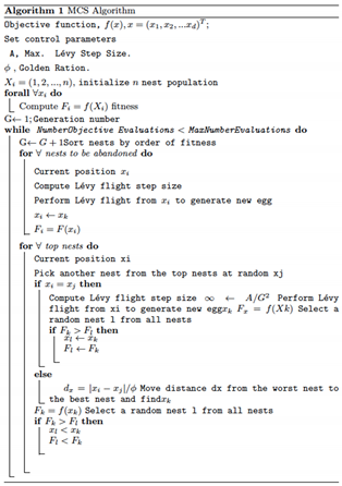
3. Modified Cuckoo Search Algorithm

Metaheuristics have been most generally applied to non-parametric problems and to other combinatorial optimization problems for which a polynomial-time solution exists but is not practical. Since their first appearance, metaheuristics have proven their efficiency in solving complex and intricate nonlinear optimization problems arising in various fields [10]. One of the most popular and used approaches is the CS algorithm. The CS algorithm is based on the cuckoo bird’s parasitic breeding behavior. This meta-heuristic is inspired by the cuckoo’s lifestyle, and it is a population-oriented stochastic global search algorithm [30]. A single egg laid by the cuckoo bird is dumped into a host bird’s nest, which is randomly selected. The host bird fails to find the cuckoo’s eggs if they show high similarity with the egg of the host bird, and then these eggs are carried to next generation. Otherwise, the host bird either abandons the nest or kills the eggs. The suitability of the nest is based on the high surviving rate of eggs.
x i ( t + 1 ) = x i ( t ) + α L é v y ( λ )
where step size α (α > 1) is related to the size of the problem. In Equation (23), xi (t+1) is created by the Lévy flight of the CS algorithm for cuckoo i [34] and ⊕ represents entry-wise multiplications. The Lévy flight-based random walk carries a very long step length which in turn explores a larger search space. Random step lengths using the Lévy distribution are represented by:
L é v y ( λ ) = t λ   where   1 < λ 3
The basic CS algorithm has two complications: premature convergence and high computational complexity. In order to improve the performance of the CS algorithm on the basis of the above analysis, Walton et al. [53] introduced the Modified Cuckoo Search (MCS) algorithm. Lévy flight modeling plays a significant role in the convergence rate control of the CS algorithm. MCS uses a new hybrid representation to take different threshold numbers from a given range, which are defined by the minimum and maximum threshold numbers. In Lévy flight CS, a faster convergence cannot be guaranteed because the search entirely depends on random walks. Consequently, to increase the convergence rate, the Lévy flight step size α must be modified. The value of α is kept either constant or 1 in the CS algorithm [37], whereas in MCS, α is decreased with the increase in the number of generations. Initially, a Lévy flight step size A of 1 is chosen, and at every generation, α = A / G is used to compute a new Lévy flight step, where G represents the generation number.
Secondly, the exchange of information does not happen between individuals, i.e., independent searches are performed in the CS algorithm. This has been modified in MCS, where information exchange among the eggs has been added to increase the speed of convergence to reach the minimum. Unlike CS, a fraction of the eggs that show the best fitness are placed into a group of best eggs. For every best egg, a second egg within the group is randomly chosen. Then, on the line that connects the above two best eggs, a new egg is generated. The inverse of the golden ratio ϕ = ( 1 + 5 ) / 2 is used to compute the distance along the line over which the new egg is positioned in such a way that it becomes closer to the egg with the best fitness. When both eggs hold the same fitness, the new egg is created at the midpoint. The use of the golden ratio shows much better performance compared to the random fraction used in CS. A local Lévy flight search carried out with a randomly picked nest has a step size of α = A / G 2 when the same egg is picked twice. Setting the fraction of nests positioned in the top nest group to 0.25 and the fraction of nests to be abandoned pa to 0.75 produces superior outcomes over various test functions. The pseudo code of the MCS algorithm is presented as Algorithm 1.
Remotesensing 13 04604 i001

4. Proposed Algorithm

A remote sensing image consists of multiple channels, where each color component carries L number of grey-levels and N number of pixels. The best threshold values are be located in [0, L−1]. Every gray level is linked to the image histogram h(i) that is a plot of the frequency of the occurrence of the ith gray pixel. The proposed algorithm represents a hybrid model formed between two stratified methods by Rényi’s entropy function and MCS. The proposed method randomly searches in the histogram as a candidate; then, the quality is evaluated using Rényi’s objective function. MCS operators are evolved on candidate strings until the optimal solutions are determined.

4.1. Multilevel Rényi’s Entropy

Consider an image I with L gray levels with values in the range 0–255. Let
p = ( p 1 , p 2 , , p n ) Δ n
Δ n = { ( p 1 , p 2 , , p n ) | p i 0 ,   i = 1 , 2 , , n ,   n 2 ,   i = 1 n p i = 1 } , which shows a set of discrete probability distributions p [9] in Equation (25). Rényi entropy is defined as [9]:
H α [ P ] = 1 1 α log 2 ( i = 1 n p i α )
for additively independent events. Here, entropy order is a positive integer α. The limiting case of Rényi entropy is when α reaches unity. The a priori Rényi entropy for each distribution [9,42,43] is represented as:
H α [ C 1 ] = 1 1 α [ ln i = 0 t 1 ( P ( i ) P ( C 1 ) ) α ] , H α [ C 2 ] = 1 1 α [ ln i = t 1 + 1 t 2 ( P ( i ) P ( C 2 ) ) α ] , , H α [ C k ] = 1 1 α [ ln i = t N + 1 L 1 ( P ( i ) P ( C k ) ) α ] ,
where
P ( C 1 ) = i = 0 t 1 P ( i ) , P ( C 2 ) = i = t 1 + 1 t 2 P ( i ) , P ( C k ) = i = t k + 1 L 1 P ( i )
The normalized histogram is represented by P(i). The best threshold values (t*= {t1, t2,..,tN}) can be obtained by the maximization of HR:
H R = H [ C 1 ] + H [ C 2 ] + + H [ C k ]
t * = a r g m a x ( H [ C 1 ] + H [ C 2 ] + + H [ C k ] )
The exhaustive search process involved in maximizing the objective function limits the application of the multilevel Rényi’s entropy as the computation complexity becomes O(LN−1). In the case of color images, Rényi’s entropy is computed for every channel of the color image. This in turn increases the computation complexity. Rényi’s entropy incorporates local information embedded in the weights and global information obtained from the gray-level histogram. Thus, Rényi’s entropy is better than the entropic correlation method or maximum entropy sum method. The objective function assesses the band subsets and provides the degree of their goodness. The performance of the system is influenced by the objective function; therefore, it needs careful determination. Consequently, an appropriate optimization algorithm needs to be selected to escape out of the local optimum and converge to the optimal global solution.

4.2. Steps for Rényi’s Entropy–MCS-Based Multilevel Thresholding

Rényi’s entropy serves as the objective criterion to reduce the complexity issues, and the MCS algorithm is implemented. The objective criterion finds the initial solution quality. At the initial step, random threshold values are generated for every candidate solution. Then, the MCS search generates new candidate solutions by exploiting solutions with objective criteria. The pre-determined rule of the MCS algorithm generates a better segmentation quality by determining the best threshold values by optimizing Rényi’s entropy. MCS avoids easy trap local optimization and causes premature convergence. Moreover, the MCS algorithm requires fewer control parameters than other meta-heuristics optimization processes. Using the operators that mimic the behavior of CS with an improved Lévy flight step size and information-exchange process, the MCS evolves solutions until it finds the optimal one. The obtained best solution is chosen and applied for image segmentation at the end of the iterative process. Below are the steps for the proposed algorithm:
Algorithm 2 Proposed Algorithm
Input:
  • Color test image to be segmented, step size (α), mutation probability value (pa), and scale factor (β), population size, number of iterations (stopping criterion), and threshold levels.
  • Step 1: Determine the optimal thresholds by maximizing the objective criterion following the MCS algorithm steps:
  • Step a: Initialize population and define the control parameters.
  • Step b: Evaluate the fitness for each nest.
  • Step c: Adjust the adaptive control parameters α and pa.
  • Step d: Generate a cuckoo egg (xi) by taking a Lévy flight from random nest.
  • Step e: Abandon some worst nests with probability pa.
  • Step f: Build new nests at new locations via Lévy flights to replace nests lost.
  • Step g: Evaluate fitness of new nests and rank all solutions.
  • Step h: If the stopping criteria is satisfied, return the best solution and finish the algorithm; otherwise, repeat again from step b.
  • Step 2: The best solutions are shown by the nests that have the best quality eggs. The set of optimal threshold values (TR, TG, and TB,) corresponds to the current best solution associated with the maximum fitness function value. The individual segmentation of each color channel leads to the corresponding threshold. The segmented image is then created by concatenating the segmented color channels.
Output:
  • A segmented color image.

5. Experimental Results and Comparison of Performances

To evaluate the performance of the proposed hybrid REMCS algorithm for the multilevel thresholding of remote sensing images, experiments were performed. The five 512 × 512 remote sensing color images shown in Figure 1 were considered for the evaluation of the proposed algorithm with different multilevel thresholding algorithms. A comprehensive evaluation of the segmentation results is presented in this section. For the analysis of the segmentation results on the test images, Rényi’s entropy, MCE, EC-Otsu, and GLCM were considered as fitness functions and evaluated using meta-heuristic optimization algorithms: MFA, MBFO, MPSO, MABC, and JADE. The remote sensing images used to evaluate the performance of the algorithms were taken from https://landsat.visibleearth.nasa.gov/ (accessed date: 1 February 2021). Multidimensional colored remote sensing images have an inherent multimodal nature because of their different bands—red (R), green (G), and blue (B). Besides, accurate and sophisticated multilevel thresholding algorithms are required for the detection and identification of the regions of interest in remote sensing images with very dense and complex features. The four thresholding levels of 2-level, 5-level, 8-level, and 12-level were used to test the robustness of the proposed REMCS and other compared algorithms. All the algorithms were implemented using MATLAB R2019b on a personal computer with a 3.4 GHz Intel core-i7 CP and 8 GB of RAM running on a Windows 10 system. The experiments were executed 30 independent times to avoid any stochastic discrepancy because of the optimization algorithm’s random nature. Since the performance of any optimization algorithm depends on the choice of the parameters, the best parametric values adopted for MFA [45], MBFO [46], JADE [47], MPSO [48], and MABC [49] from the respective literature of the algorithm are listed in Table 1. The population size was set as 25 and the number of iterations was set as 100 to keep fairness when comparing the performances among MCS and other bio-inspired algorithms.

5.1. Fidelity Parameters for Quantitative Evaluation of the Results

As the segmentation level increases, more classes with distinct characteristics are acquired. These characteristics maintain the local features within the original image. It is impossible to determine the performance of each algorithm with the human eye for the same segmentation level, especially when a complex image with multiple objects is used. Consequently, the segmented image quality requires evaluation using some specific metrics. To carry out a comprehensive assessment of the performance of the algorithms, computation time (in seconds), mean square error (MSE), peak signal-to-noise ratio (PSNR), structural similarity (SSIM), and feature similarity (FSIM) indexes are reported in Table 2, Table 3, Table 4, Table 5, Table 6, Table 7, Table 8, Table 9, Table 10 and Table 11. The values represent averages computed over four levels (2, 5, 8, and 12) for each of the five different test images shown in Figure 1. Table 12 shows the Wilcoxon statistical test used to judge the significance of the proposed algorithm.

5.1.1. Computation Time (in Seconds)
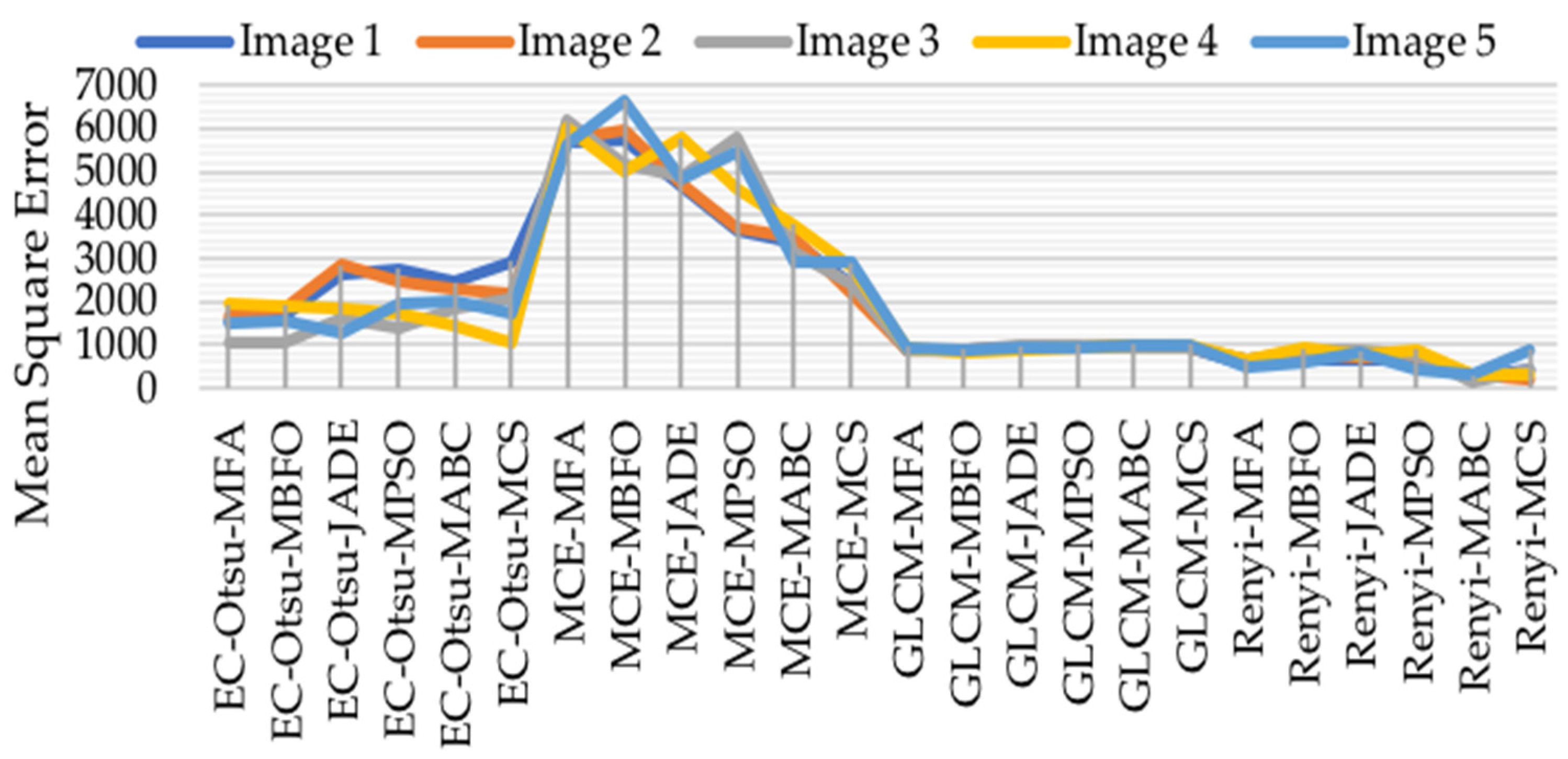
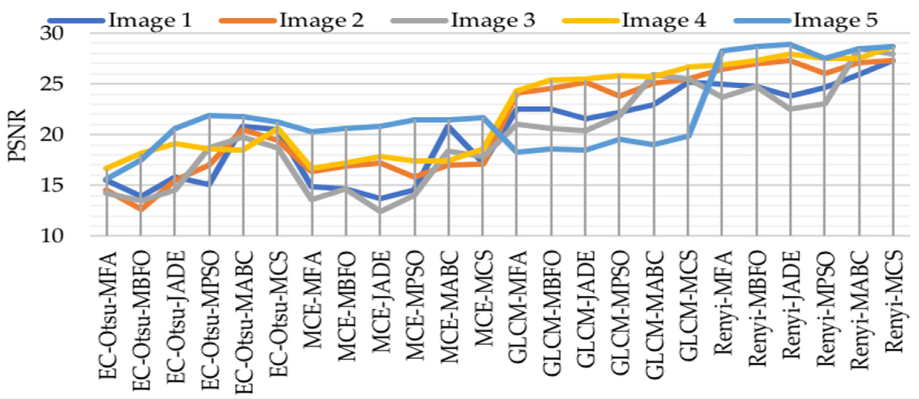
The complexity of any algorithm influences its computation time. The mathematical structure of any algorithm and the objective function used defines the complexity of that algorithm. As a result, computation time becomes an essential factor to determine the efficiency of an algorithm. The time involved to generate the segmented image is directly proportional to the algorithm’s complexity.

5.1.2. PSNR and MSE

PSNR and MSE determine the accuracy of the segmentation algorithm, defined as:
M S E = 1 M N i = 1 M j = 1 N [ I ( i , j ) I ˜ ( i , j ) ] 2
P S N R = 10 log 10 ( 255 2 M S E )
where M and N represent the image size, I is the input image to be segmented, and Ĩ is the output image at pixel position (i,j) after segmentation at a given thresholding level. A high PSNR and a low MSE are desired to indicate the good performance of an algorithm.

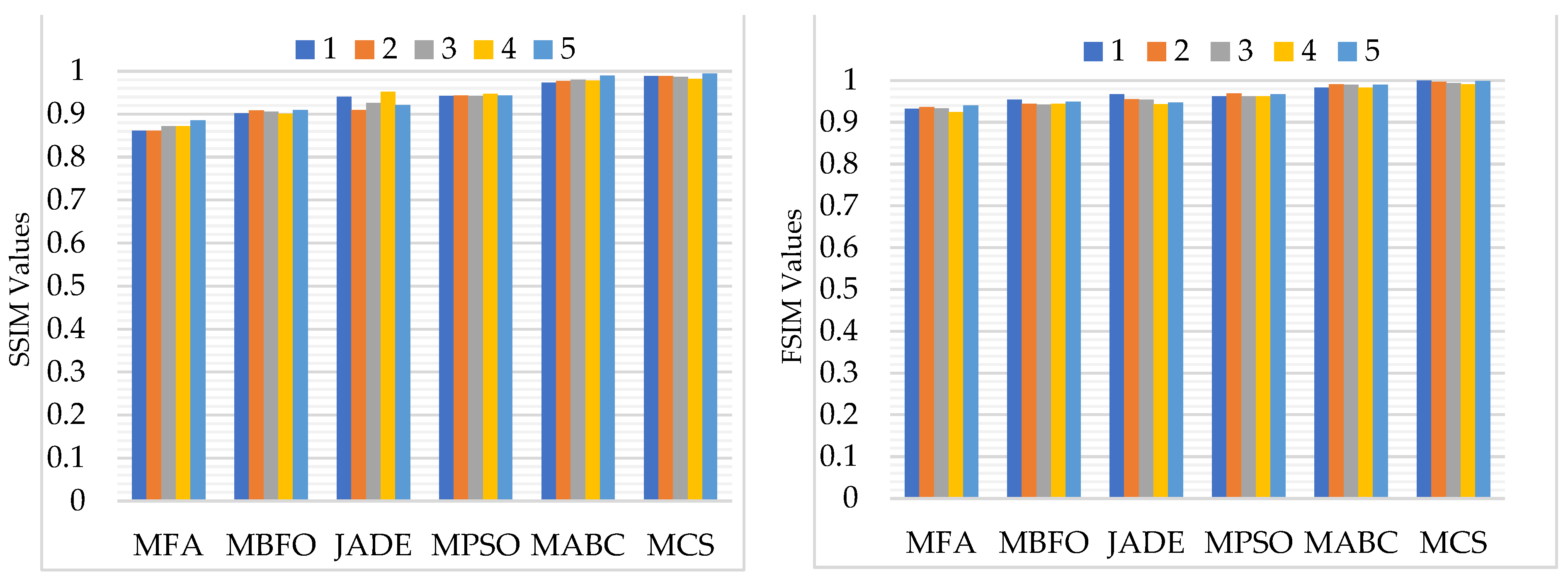
5.1.3. SSIM and FSIM

The global similarity between the input and the segmented output image can be measured by using two parameters: SSIM and FSIM. FSIM indicates how well the features are preserved after the processing of the image. This is significant in the classification systems for remote sensing images. SSIM indicates the visible structures of the test image that are likely to be passed over the segmented image. SSIM is a parameter used to assess the quality of the segmented image and is based on structural information degradation. The SSIM compares the input and segmented output structures using [15,39]:
SSIM ( x , y ) = ( 2 μ x μ y + U 1 ) ( 2 σ x y + U 2 ) ( μ 2 x + μ 2 y + U 1 ) ( σ 2 x + σ 2 y + U 2 )
The mean intensity of image x and y is given by µx and µy, respectively. The standard deviations of x and y are given by σx and σy, respectively. The local sample correlation coefficient between x and y is given by σxy. The constants—U1 = U2 = 0.065—are used to circumvent any instability closer to zero. For multichannel images,
SSIM = c SSIM ( x c , y c )
where xc and yc represent the cth channel of the input image and segmented output image, respectively, where c (i.e., c = 1, 2, 3 in true color RGB images) shows the channel number.
FSIM computes the feature similarity between the input and segmented images [39] as follows:
FSIM = X Ω S L ( X ) P U m ( X ) X Ω P U m ( X )
where the entire image is indicated by Ω and SL(x) shows the similarity between the segmented output image and input image. For multichannel images,
FSIM = c FSIM ( x c , y c )
SSIM and FSIM vary between 1 and 0, where 1 indicates the maximum similarity or a high segmentation quality and 0 represents the minimum similarity or a poor segmentation quality of the output. The fidelity parameters for each channel of the multichannel images are computed separately, and their averages can be taken as the final values.

5.2. Comparison Using the Otsu Energy (EC-Otsu) Method as an Objective Function

The results obtained by using the MFA [45], MBFO [46], JADE [47], MPSO [48], MABC [49], and MCS [29] with the EC-Otsu method as a fitness function are shown in Table 2, Table 3 and Table 4, and Figure 2, Figure 3 and Figure 4 show their graphical representations. Figure 5 shows a visual comparison of the results. Detailed tables indicating the results computed over each of the segmentation levels (2, 5, 8, and 12) are shown in Appendix Table A1, Table A2 and Table A3. The analysis of the algorithms is discussed below.

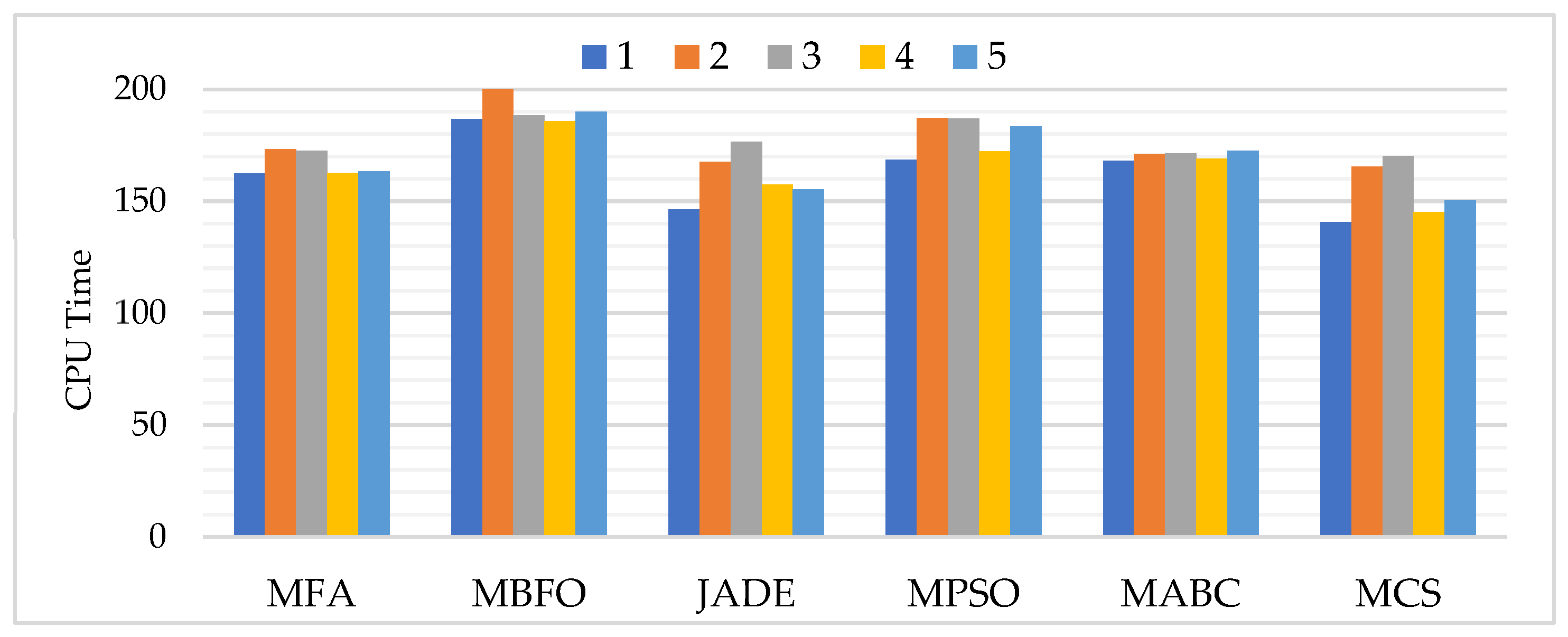
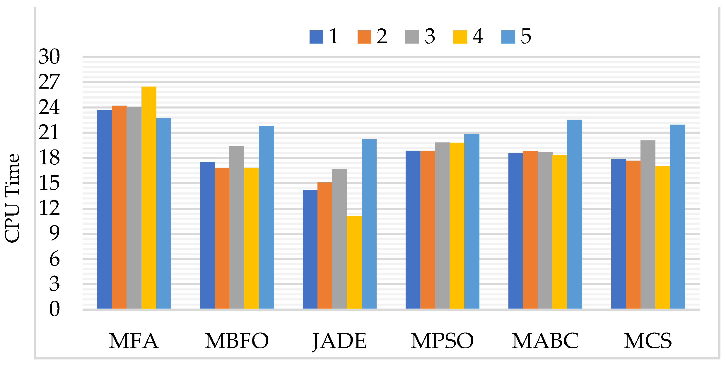
5.2.1. Assessment Based on Computation Time (CPU Time)

Figure 2 shows the graphical analysis of average CPU time computed using the EC-Otsu-based algorithms. Table 2 shows the quantitative results. The MCS algorithm presented the best computation time. In terms of efficiency, MBFO took the largest time due to its complex strategy of searching the optimal solutions. The complexity of this method depends on the mathematical modeling of the objective function, as well as the architecture and search strategy of the optimization algorithms. Therefore, different algorithms lead to different results. For EC-Otsu, the optimization algorithms in terms of increasing time complexity could be arranged as MCS < JADE < MFA < MABC < MPSO < MBFO.

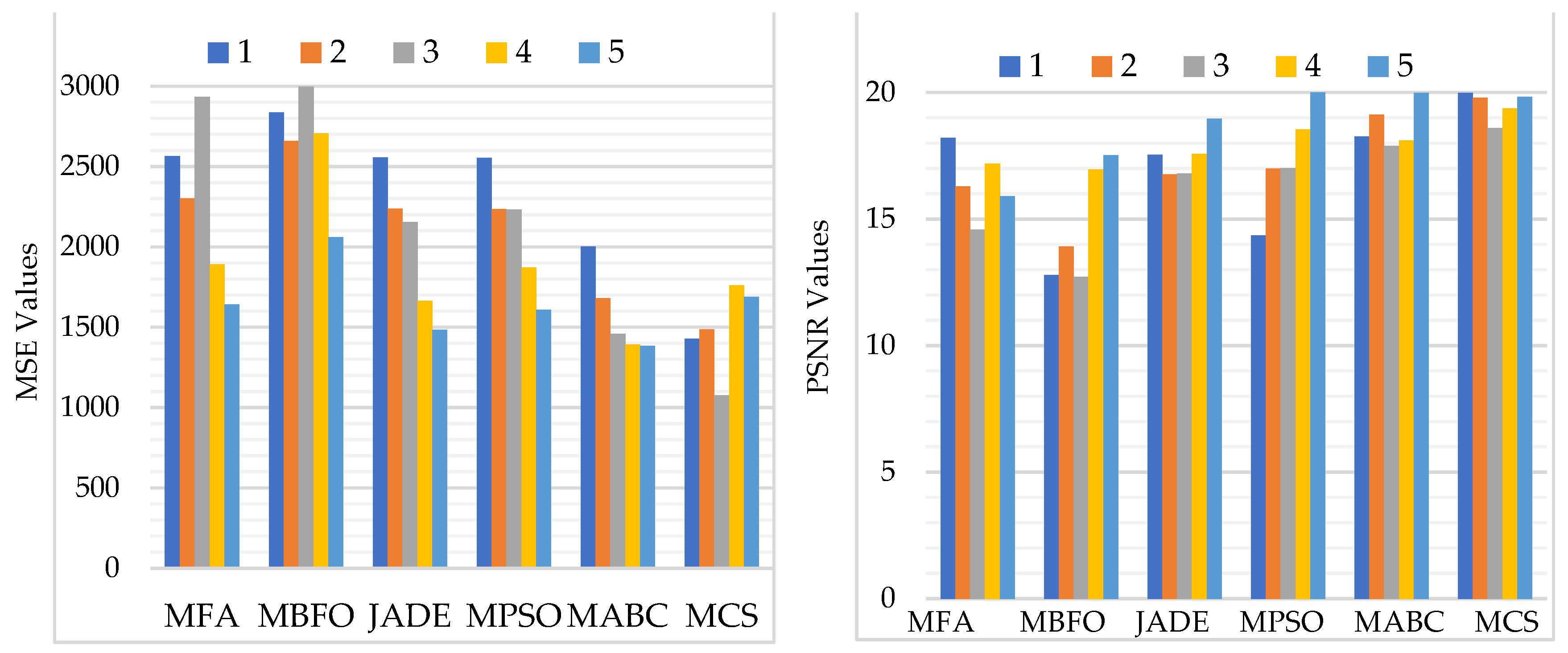
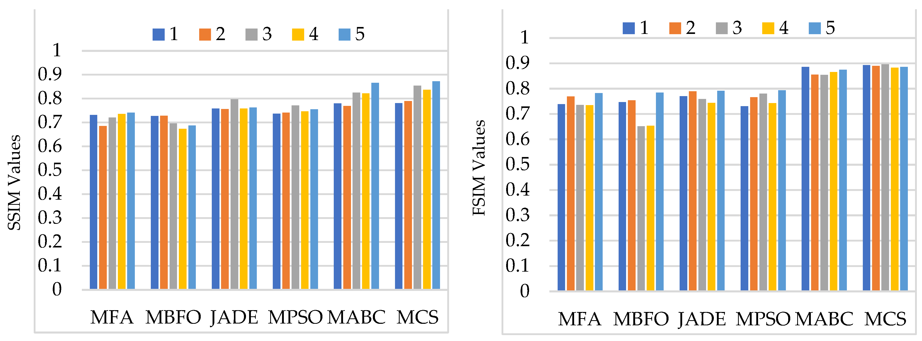
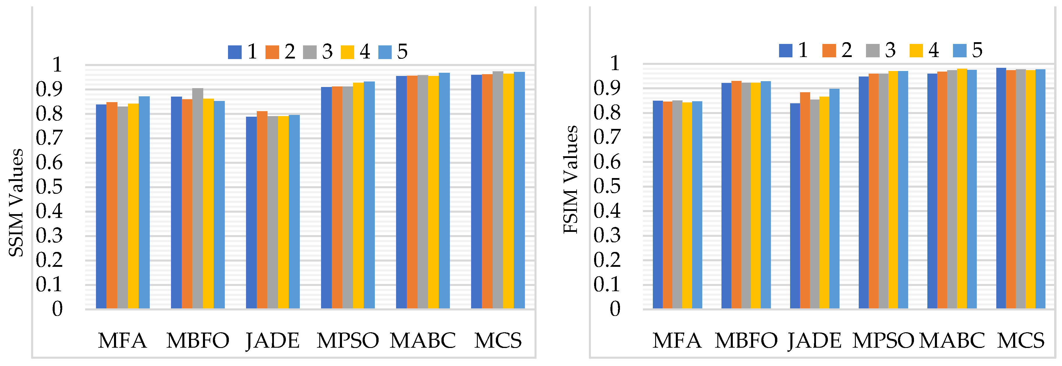
5.2.2. Assessment Based on PSNR, MSE, SSIM, and FSIM

Figure 3 shows a graphical comparison of the average PSNR and MSE computed using EC-Otsu-based algorithms. Table 3 shows a quantitative comparison. According to the results, the average PSNR and MSE values for the MCS algorithm were the best. In other algorithms, JADE obtained somewhat better values, while the results of MABC and MPSO were nearly equal. MBFO obtained the lowest PSNR values. In terms of increasing PSNR and decreasing MSE values, the order of the algorithms was MBFO < MPSO < JADE < MABC < MFA < MCS.
Figure 4 shows a graphical comparison of the average SSIM and FSIM computed using EC-Otsu-based algorithms. Table 4 shows the quantitative results. The maximum SSIM and FSIM were obtained in the case of MCS, followed by JADE, MABC, MPSO, MFA, and MBFO, which indicates the excellent optimization ability of MCS in comparison to the other metaheuristic approaches. The substantial difference between the performances indicates that the segmentation performance obtained by the MBFO, JADE, and MPSO algorithms deteriorated due to the randomness introduced in the selection of the initial population. Moreover, the Lévy flight strategy of MCS had a greater influence on the optimization ability of the algorithm. In terms of increasing SSIM and FSIM values, the order of the algorithms was MBFO < MFA < MPSO < JADE < MABC < MCS.

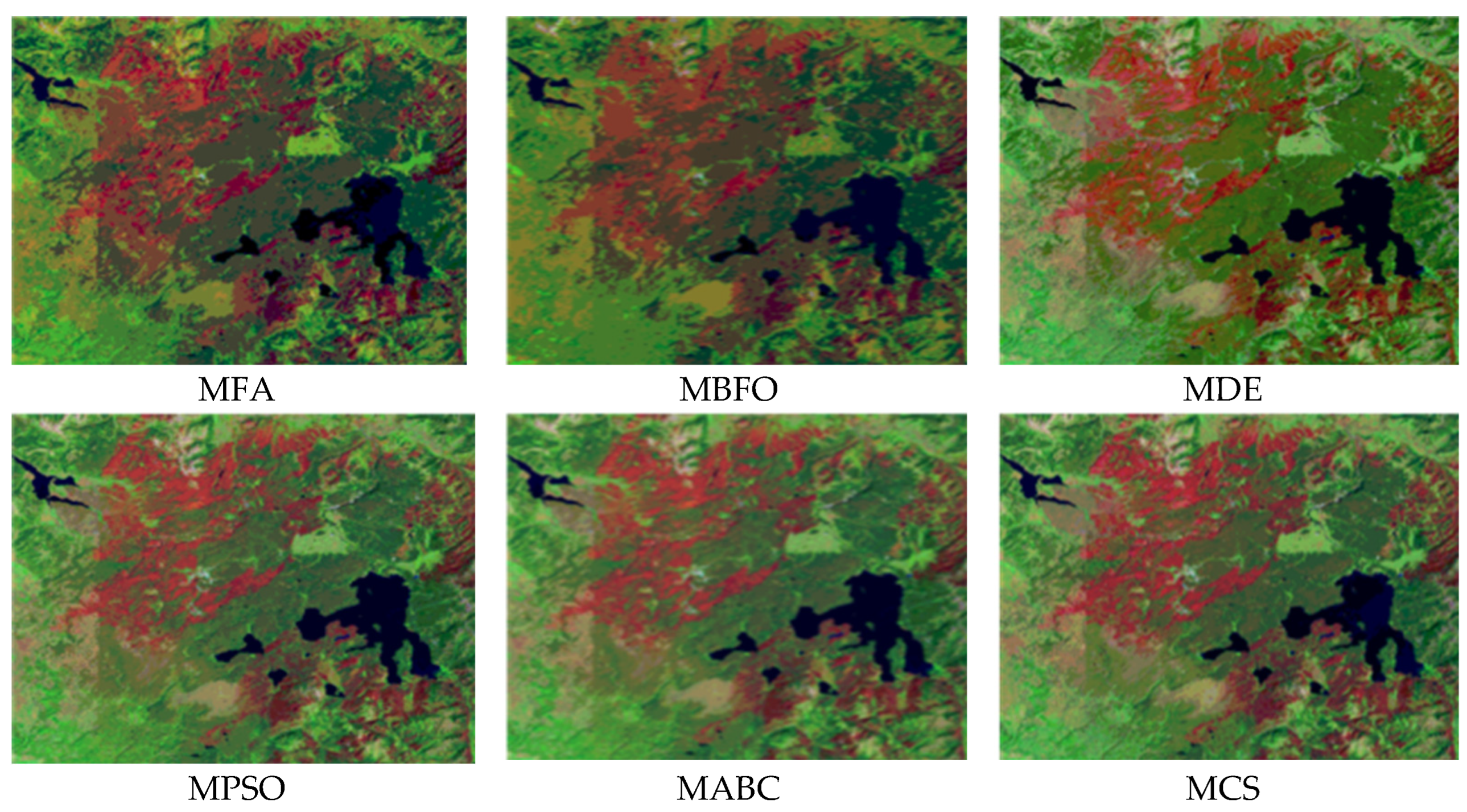
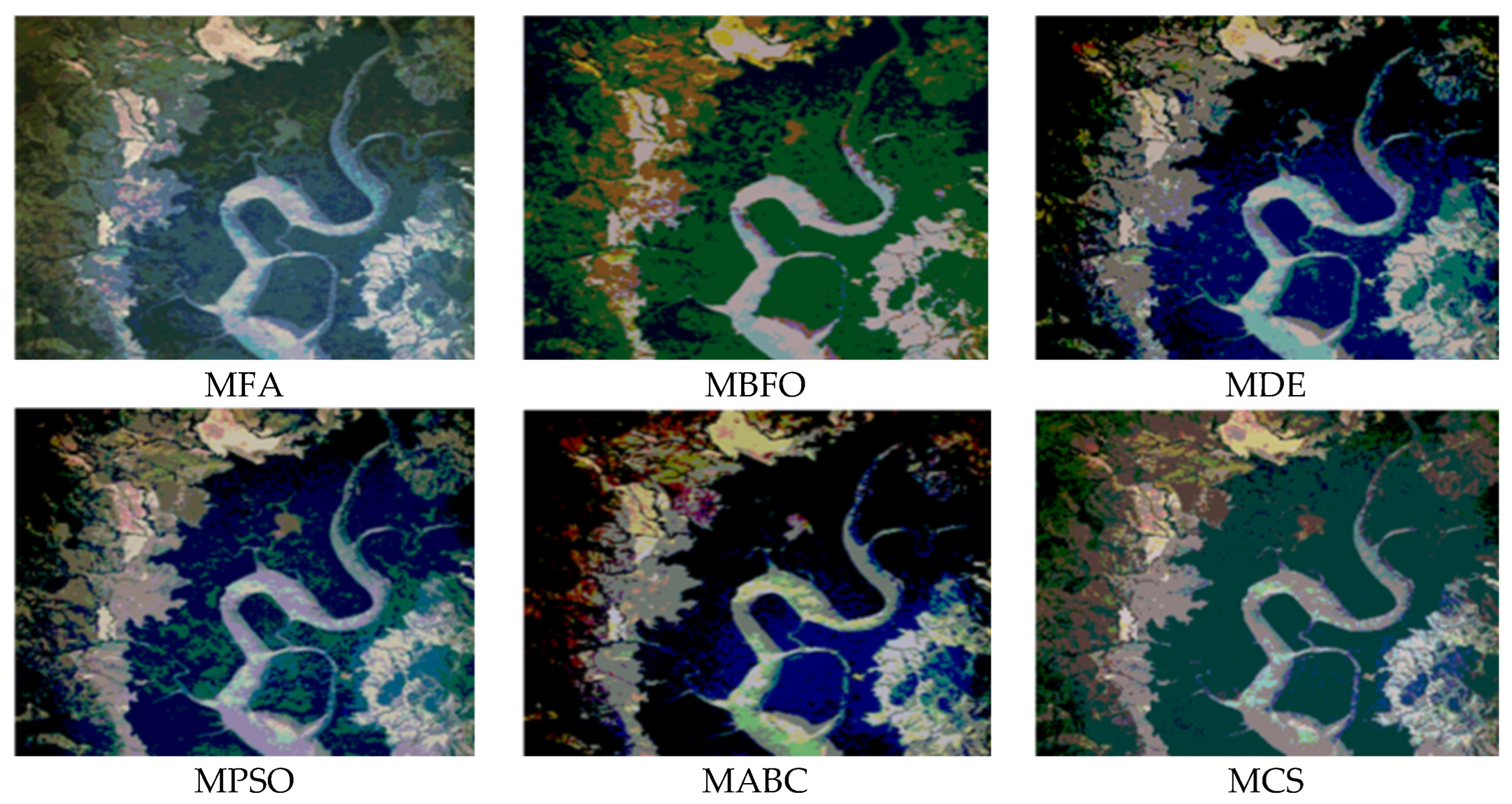
5.2.3. Visual Analysis of the Results

Figure 5 shows the segmented outputs using the EC-Otsu method. MCS obtained the best segmented output, but MBFO was not able to properly distinguish the pixels among different classes based on their gray levels. The obtained results were not satisfactory. The rest of the algorithms obtained good results at higher thresholding levels. At lower thresholding levels, the segmented output was not very satisfying when using MFA. Generally, as the thresholding level increased, the image quality also improved. From the figure, it can be seen that MCS exhibited excellent optimization performance and searching ability, making it the best choice to solve the segmentation problem.

5.3. Comparison Using MCE Method as an Objective Function

The results obtained using MABC, MPSO, JADE, MFA, MBFO, and MCS using the MCE method as a fitness function are shown in Table 3, Table 5 and Table 6, and Figure 6, Figure 7 and Figure 8 show the average values computed over four different threshold levels (2, 5, 8, and 12). Figure 9 shows a visual comparison of the results. Detailed tables indicating the results computed over each of the segmentation levels (2, 5, 8, and 12) are shown in Table A1, Table A4, and Table A5. The analysis of the algorithms is discussed below.

5.3.1. Assessment Based on Computation Time (in Seconds)

Multilevel MCE was maximized using different optimization algorithms to obtain a segmented image. Figure 6 shows the graphical comparison of the average CPU time computed using MCE-based algorithms. Table 3 shows the quantitative results. According to the obtained results, the MCS algorithm was the fastest due to the use of few tuning parameters. JADE also obtained faster results than the MABC and MPSO, which were trapped into local minima. Other algorithms also performed well in the case of MCE. For MCE, the optimization algorithms in terms of increasing time complexity could be arranged as MCS < JADE < MFA < MPSO < MABC < MBFO.

5.3.2. Assessment Based on PSNR, MSE, SSIM, and FSIM

Figure 7 shows a graphical comparison of the average MSE and PSNR computed using the MCE-based algorithms. Table 5 shows the quantitative values. The best results were obtained using the MCS algorithm, followed by ABC and DE. The PSNR and MSE values computed using MBFO were nearly the same as those obtained using MFA, whereas the JADE outputs followed those of the MCS. The high PSNR indicated the better segmentation quality. In terms of increasing PSNR and decreasing MSE values, the order of the algorithms was JADE < MPSO < MFA < MBFO < MABC < MCS.
Figure 8 shows a graphical comparison of the average SSIM and FSIM computed using MCE-based algorithms. Table 6 shows the quantitative results. Both SSIM and FSIM are the essential parameters in the analysis of the segmentation quality of any algorithm. In the case of MCE, SSIM and FSIM were at maximum when using MCS. The other algorithms showed fair results. JADE obtained good results. The performance of MBFO and MFA was good at lower threshold levels. In terms of increasing SSIM and FSIM values, the order of the algorithms was JADE < MPSO < MFA < MBFO < MABC < MCS.

5.3.3. Visual Analysis of the Results

From Figure 9, it can be seen that the MBFO and MFA failed to be efficient in accurately finding the threshold values. This led to poor segmentation in some of the cases. The average computed values show that MCS resulted in good outputs. Furthermore, the searching ability of the CS algorithm was improved by adaptively adjusting the Lévy flight step size. An adaptive step size led to significantly improved solution quality, overcame premature convergence, and helped the algorithm to come out of local optima. This resulted in more reliable and stable optimization performance.

5.4. Comparison Using GLCM as an Objective Function

The average segmentation results by using MABC, MPSO, MDE, MFA, MBFO, and MCS with GLCM methods as a fitness function are quantitatively shown in Table 7, Table 8 and Table 9 and graphically shown in Figure 10, Figure 11 and Figure 12. Figure 13 shows a visual comparison of the results. Detailed tables indicating the results computed over each of the segmentation level (2, 5, 8, and 12) are shown in Table A6, Table A7 and Table A8. The analysis of the algorithms is discussed below.

5.4.1. Assessment Based on Computation Time (in Seconds)

The GLCM objective criterion is based on second-order statistics. This method was maximized to achieve thresholding results. Figure 10 shows a graphical analysis of the average CPU time. Table 7 shows a quantitative comparison of the average values. The results obtained using GLCM showed the efficiency of most of the optimization algorithms, as shown in Figure 10 and Table 7. In GLCM, in terms of increasing computation time, the algorithms could be arranged as JADE < MBFO < MCS < MABC < MPSO < MFA.

5.4.2. Assessment Based on PSNR, MSE, SSIM, and FSIM

Based on the average PSNR and MSE values in Figure 11 and Table 8, MCS had the best performance so far. In terms of the accuracy measured using PSNR, MABC, MBFO, JADE, and MFA showed satisfying performance. MPSO, however, was trapped into local minima, which affected its searching efficiency. MSE was the worst with the MCS algorithm. For GLCM, in terms of increasing PSNR and decreasing MSE values, the algorithms could be arranged as JADE < MBFO < MFA < MPSO < MABC < MCS.
Figure 12 and Table 9 report the average computed SSIM and FSIM. The complete analysis of the GLCM-based optimization techniques shows that MCS achieved optimal average values in comparison to other cases for most of the considered images. In terms of increasing SSIM and FSIM, the algorithms could be arranged as JADE < MFA < MBFO < MPSO < MABC < MCS.

5.4.3. Visual Analysis of the Results

A comparison of the segmented images in Figure 13 shows that MCS had the best segmented outputs, even though the segmented image looked under-segmented in some cases. MPSO resulted in poorly segmented images at lower and higher threshold levels. JADE was better; however, it was not as good as MCS. JADE showed the same results as the MCS for some cases. MBFO also presented poorly segmented results in a few cases.

5.5. Comparison Using Rényi’s Entropy as an Objective Function

In this section, the quantitative analysis of different optimization algorithms using Rényi’s entropy as a fitness function is shown. The performance was evaluated using the average values of the metrics over four segmentation levels (2, 5, 8, and 12), as shown in Table 7, Table 8 and Table 9 and Figure 14, Figure 15 and Figure 16. Figure 17 shows a visual comparison of the results for each segmentation technique. Detailed tables indicating the results computed over each of the segmentation levels (2, 5, 8, and 12) are shown in Table A6, Table A9, and Table A10. The analysis of the algorithms is discussed below.

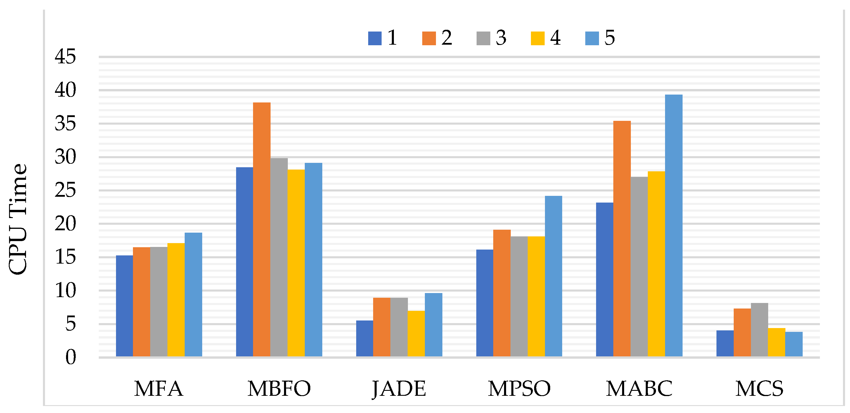
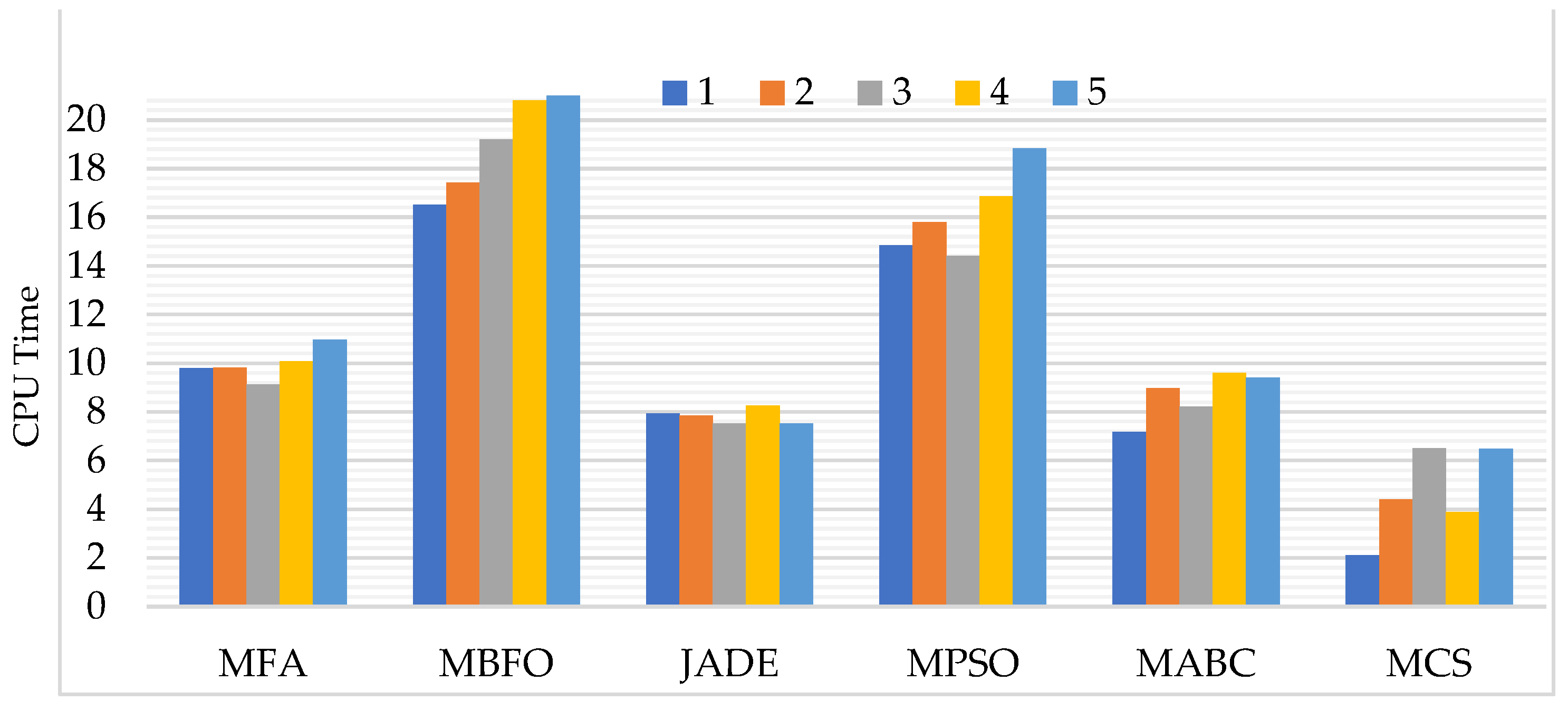
5.5.1. Assessment Based on Computation Time (in Seconds)

Based on the average computation time results recorded in Table 7 and shown in Figure 14, MCS was the most suitable algorithm to use with Rényi’s entropy for producing an output in less time. The MCS more efficiently obtained results compared to other algorithms. JADE showed satisfactory performance, and the computation complexity of MABC was almost similar to that of JADE. On the other hand, the performance of MBFO was inferior to that of MPSO and MFA. For Rényi’s entropy, in terms of increasing CPU time, the algorithms could be arranged as MCS < JADE < MABC < MFA < MPSO < MBFO.

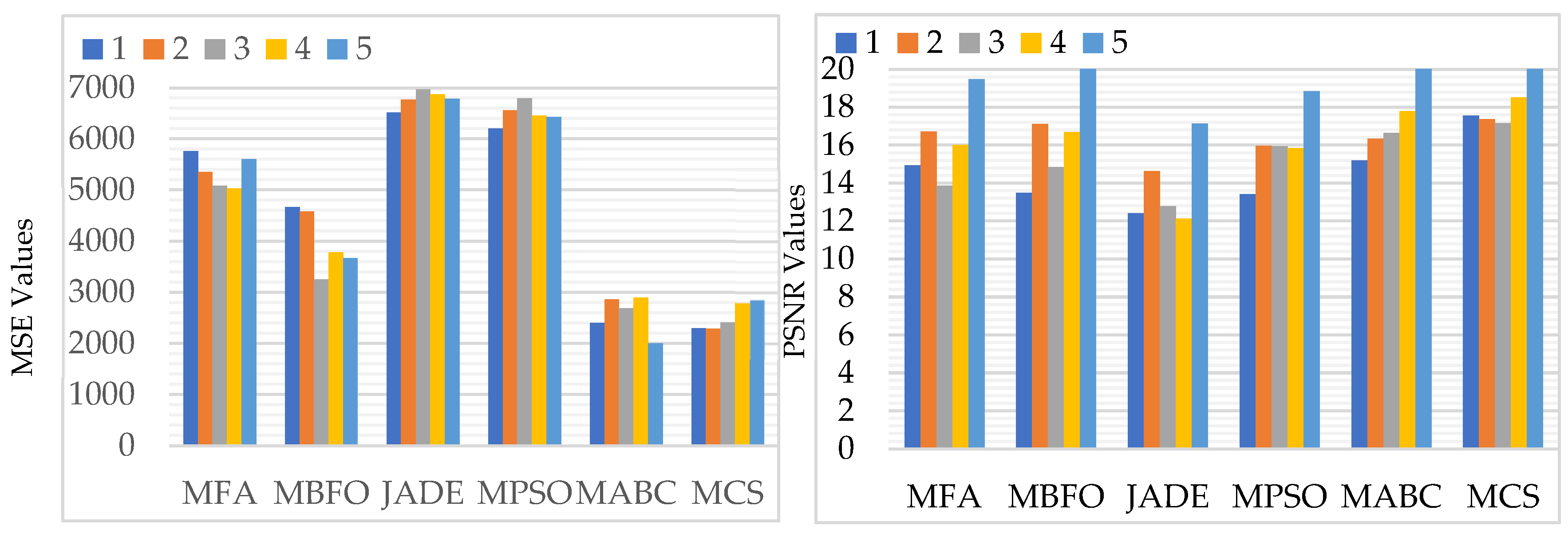
5.5.2. Assessment Based on PSNR, MSE, SSIM, and FSIM

Figure 15 shows a graphical comparison of the average PSNR and MSE values computed using Rényi’s entropy based on MCS, MABC, MPSO, JADE, and MFA. Table 10 shows the quantitative results. For each of the algorithms, it can be seen that the PSNR value improved as the thresholding level increased. On the other hand, the MSE value decreased. This indicates that the segmented results better resembled the original image when increasing the thresholding level. For Rényi’s entropy, in terms of increasing PSNR and decreasing MSE values, the algorithms could be arranged as MFA < MBFO < JADE < MPSO < MABC < MCS.
Figure 16 shows a graphical comparison of the average SSIM and FSIM values computed using the Rényi’s entropy-based algorithms. Table 11 shows the quantitative results. The MCS-based results were superior to those of other compared algorithms. Here, MABC again showed better performance than the rest of the optimization algorithms, which are compared in Table 10. For Rényi’s entropy, in terms of increasing SSIM and FSIM values, the algorithms could be arranged as MFA < MBFO < JADE < MPSO < MABC < MCS.
The proposed REMCS algorithm obtained superior results in most of the cases than other recently developed modified metaheuristics algorithms (MABC, MFA, MBFO, and MPSO). This occurred because every image had diverse features characterizing a specific optimization problem. In addition, the random nature of these algorithms generated some fluctuations in the segmentation outcomes. For instance, if a thresholding value was obtained using a metaheuristic that was not suitable, it generated a segmented image that was not optimal. Therefore, in terms of Rényi’s entropy, it can be seen that MCS produced the best results. Unlike other optimization algorithms, MCS increased the probability of obtaining the global optimum because of its well-balanced exploration and exploitation stages.

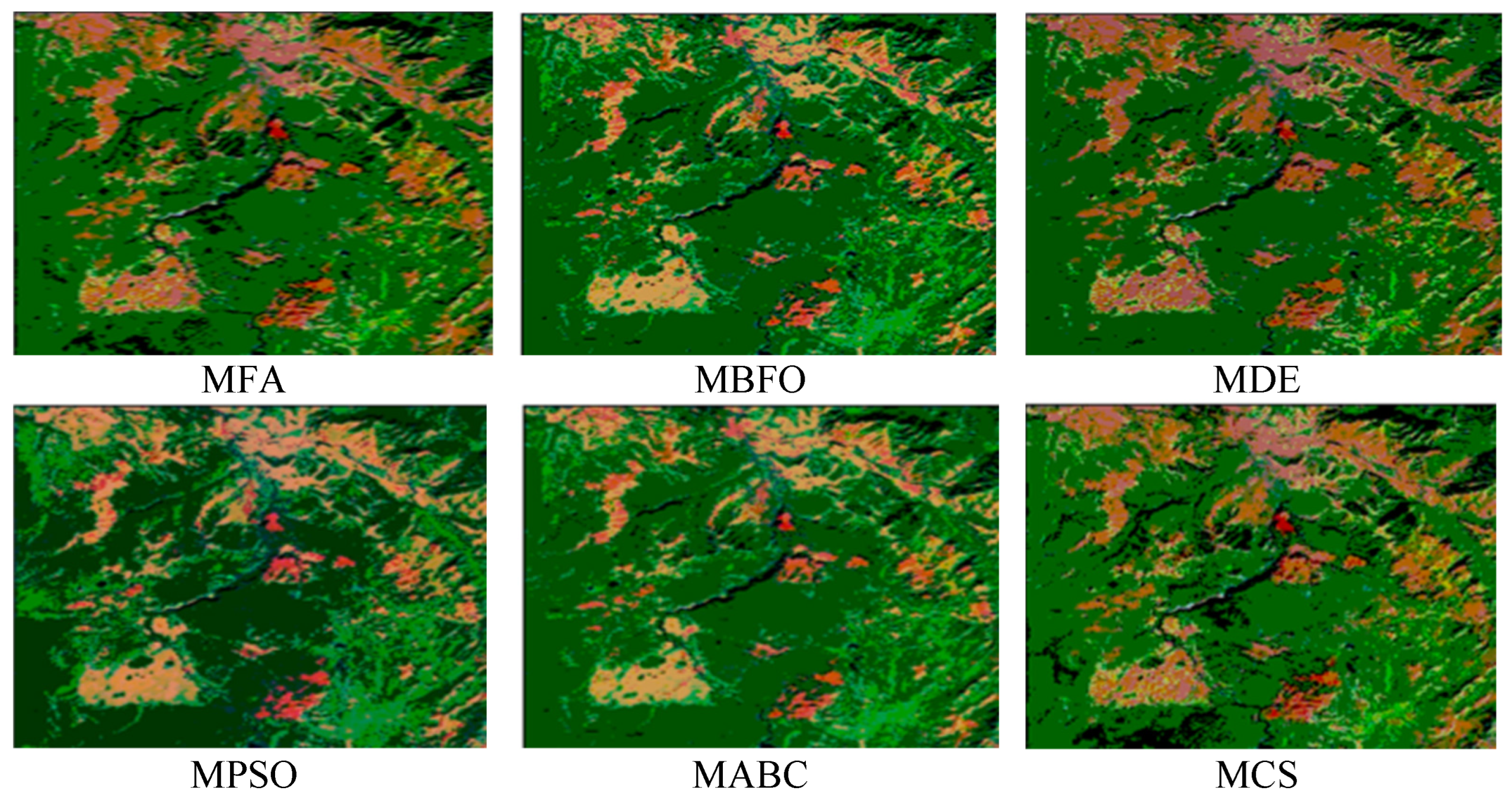
5.5.3. Visual Analysis of the Results

Figure 17 shows the visual results of the proposed and other compared techniques. The segmentation was visually best for the proposed algorithm. The performances of the algorithms are visually shown by their qualitative results. MABC presented better results than MPSO. The JADE and MBFO algorithms under-segmented the outputs because of their poor capability of accurately locating thresholding levels so that they could separate the pixels into homogenous regions. Figure 6 shows that as the thresholding level increased, the segmentation quality also improved.

5.6. Comparison between Rényi’s Entropy, Energy-Otsu Method, MCE, and GLCM

In this section, different objective criteria are compared on the basis of the quantitative outcomes reported in Table 2, Table 3, Table 4, Table 5, Table 6, Table 7, Table 8, Table 9, Table 10 and Table 11 with graphical and visual representations in Figures 19–22. Qualitative results are shown in Figure 23.

5.6.1. Assessment Based on Computation Time (in Seconds)

The average computation times obtained using Rényi’s entropy, the EC-Otsu method, MCE, and GLCM are given in Table 2 and Table 7 and shown in Figure 18. Rényi’s entropy uses global information obtained from the gray-level histogram and local information. Because the objective criteria had strong significance in locating the thresholds, the mathematical modeling of Rényi’s entropy provided good results. After Rényi’s entropy, GLCM presented the fastest results due to the use of the second-order statistics. Energy-Otsu appeared to be the most inefficient algorithm in terms of determining the optimal thresholds. The major drawback of the EC-Otsu method is the high processing time it requires to perform segmentation due to the time required for the computation of the energy function. In Table 2 and Table 7, it is clear that the computation time of each test image via the proposed approach was minimum. The algorithms based on EC-Otsu require large computation times.

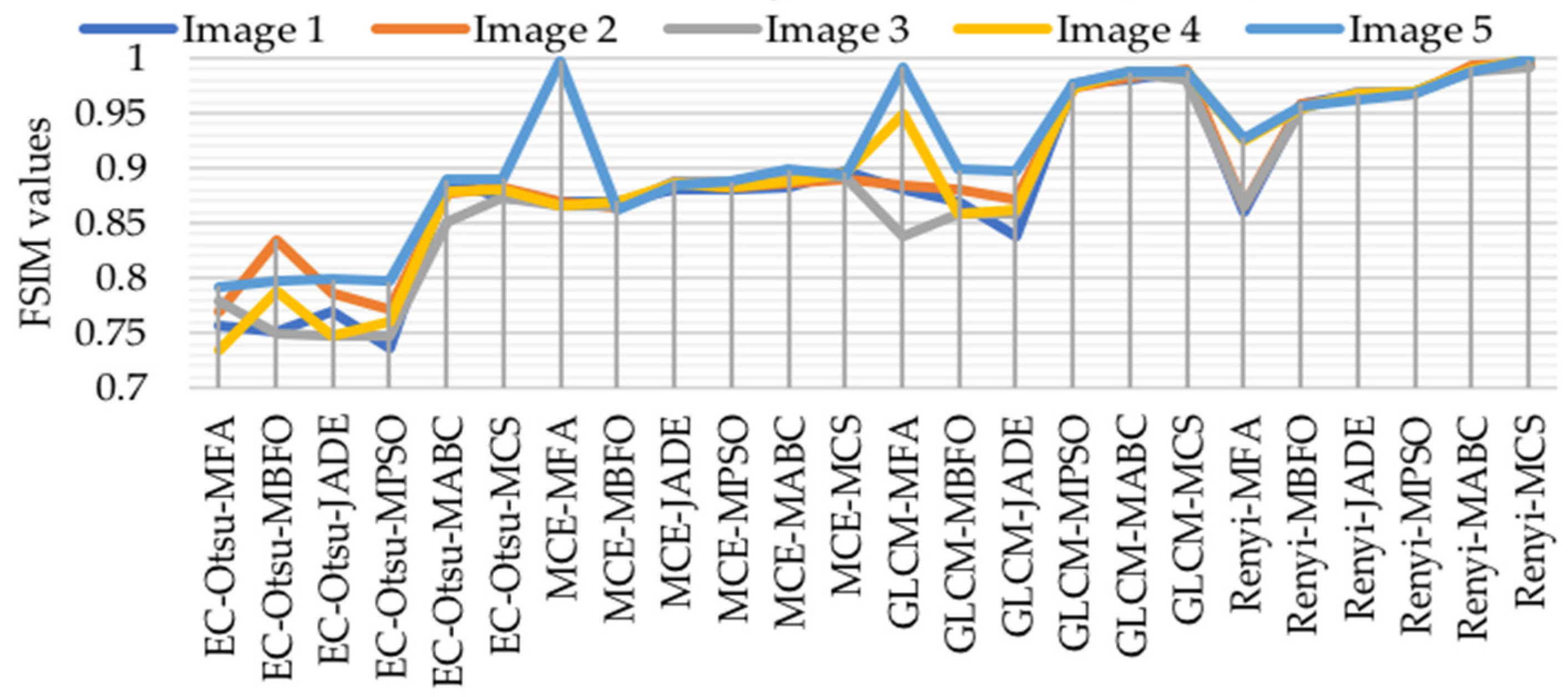
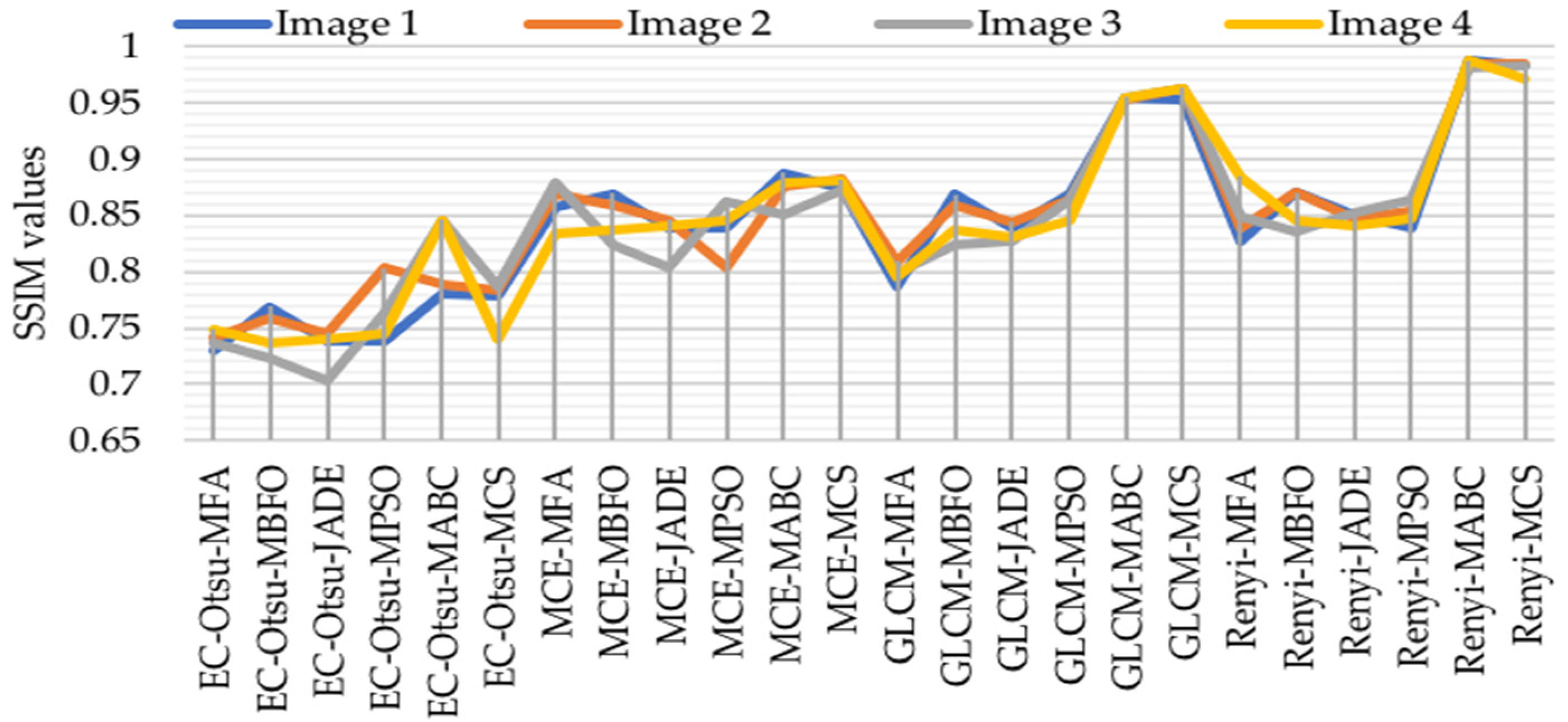
5.6.2. Assessment Based on PSNR, MSE, SSIM, and FSIM

Table 3, Table 5, Table 8 and Table 10 report the PSNR and MSE for each of the four objective functions used. Graphically, the quantitative results are shown in Figure 19 and Figure 20. Rényi’s entropy works with the information of the image’s histogram, which usually presents multi-modality and local sub-optima configurations. Moreover, the architecture of Rényi’s entropy more efficiently explores the search space. Under such a scenario, the population-based MCS algorithm generated accurate and near-optimal threshold values compared to all other optimization techniques. In contrast, GLCM, EC-Otsu, and MCE only offered information about how the intensity values were distributed in different regions. These could be verified from qualitative metrics as reported in Table 2, Table 3, Table 4, Table 5, Table 6, Table 7, Table 8, Table 9, Table 10 and Table 11 and shown graphically in Figure 19, Figure 20, Figure 21 AND Figure 22. The EC-Otsu model is good when accuracy is of major concern due to the mathematical model of EC-Otsu and the properties of EF. The MCE approach can also be considered for multilevel thresholding, but this objective function requires a large number of evaluations and iterations to give optimal values. GLCM is an average method when accuracy is the major concern; the method integrates intensity and edge magnitude information. Table 4, Table 6, Table 9 and Table 11 compare the performances of objective functions in terms of similarity measures such as SSIM and FSIM. The results are shown graphically in Figure 21 and Figure 22.

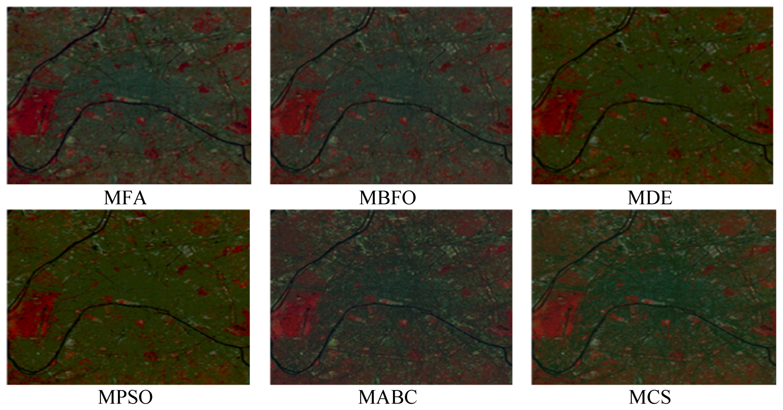
5.6.3. Visual Analysis of the Results

A comparison of the segmented test images in Figure 23 shows the proposed algorithm presented much better results than the other compared algorithms. Comparing the results reveals that in the case of the MCS algorithm, Rényi’s entropy showed the best performance due to its balanced exploration–exploitation and noteworthy optimization capability. This also indicates that the segmented output using REMCS was of high quality in terms of details and information, as the entropy provided the average information content of the image; in other words, the reason for its high precision was the use of a powerful hybrid algorithm. The results of MCE followed Rényi’s entropy. EC-Otsu and GLCM performed fairly as well at classifying pixels for higher levels. In the cases of MABC and MPSO, Rényi’s entropy exhibited better segmentation. GLCM and EC-Otsu improperly segmented pixels. MCE showed somewhat better outputs than when using both MCS and JADE. EC-Otsu showed poor results with MFA and MBFO.

5.7. Statistical Analysis Test

This section discusses a rank-based statistical analysis of the performance assessment of the presented multilevel thresholding techniques and included optimization algorithms. The assessment technique for the non-parametric statistical hypotheses—namely, the Wilcoxon signed-rank test—measures the capability of the proposed approach compared to other considered approaches. These statistical results were obtained for 20 cases used in the experiment (five images and four different threshold levels). The analysis was performed using a 5% significance level over PSNR values to check the substantial variance between the proposed approach and other algorithms. In the Wilcoxon test, null hypotheses indicate no considerable change between the PSNR values of compared techniques, while the alternative hypothesis indicates a remarkable change. An h value of 1 means the null hypothesis can be rejected at a 5% level of significance, while an h value of 0 indicates that the null hypothesis cannot be rejected. If p < 0.05 (5% significance level), there is strong evidence against the null hypothesis, demonstrating that the better final objective function values achieved by the best algorithm in each case are statistically significant and have not occurred by chance. In Table 12, the p-values produced by Wilcoxon’s test results for Rényi entropy and other entropy functions (GLCM, MCE, and EC-Otsu) using MCS as a control algorithm are compared over the PSNR. The p-values were less than 0.05 (5% significance level) for the majority of cases. In the experiments using Rényi’s entropy as an objective function, the MCS algorithm presented better results in 18 out of 20 total cases when compared to the MPSO, MFA, and JADE algorithms, and it produced better results in 20 out of 20 total cases when compared to the MABC and MBFO algorithms.

6. Conclusions and Future Work

6.1. Conclusions

In this paper, we present a new color image multilevel thresholding technique using a multilevel Rényi’s entropy function and MCS algorithm. This method is a hybrid between the MCS algorithm and Rényi’s entropy model for remote sensing image segmentation. Remote sensing images are by nature multi-dimensional and multimodal with dense characteristics and uncertainties, which increases the computation complexity of determining the best thresholds with an exhaustive search procedure. Since the parameter estimation in the segmentation algorithm is typically a nonlinear optimization problem, the parameters used in Rényi’s entropy are determined using MCS. The results of the proposed REMCS algorithm were compared with modified versions of different popular bio-inspired optimizations (MFA, MBFO, JADE, MPSO, and MABC). To justify the performance of the proposed algorithm, other popular entropy models (GLCM, EC-Otsu, and MCE) were also included.
Multilevel thresholding is an extremely difficult problems to overcome because, upon increasing segmentation levels, the difficulty exponentially increases. In terms of the accuracy measured by PSNR and MSE values, REMCS showed significantly better results than the other methods. REMCS was successful in achieving high SSIM and FSIM values at all segmentation levels, while other algorithms failed when the level increased. To assess the significant differences between the methods, comprehensive statistical tests (Wilcoxon’s rank sum test) were used, indicating the significant differences between the proposed algorithms. The experimental results based on the evaluation of the satellite images verified the performance of the proposed algorithm on the low-level and high-level thresholds. The complete analysis revealed that the proposed REMCS produced the best value for a maximum number of fidelity parameters compared to the other techniques. REMCS preserved the fine details in the segmented images, as is necessary for the analysis of remote sensing imageries. A remarkable characteristic of the proposed algorithm was due to Rényi’s entropy, which was derived from the gray-level distribution of an image and hence provided better results. The numerical and visual analyses of the segmentation outcomes revealed the proficiency, fast convergence, and robustness of the proposed algorithm compared to the other meta-heuristic-based segmentation algorithms.

6.2. Future Work

The proposed method was found to significantly increases segmentation accuracy without affecting the original color and details of the input image. However, a limitation is that the histogram fails to consider the spatial contextual information of the image, which affects the accuracy of segmentation. To overcome such drawbacks, future works in this area will focus on improving the proposed algorithm by integrating contextually fused objective criteria. On the other hand, the approach does not need any training or learning phases, which generalizes its applicability to a diversified set of images. Hence, it can be explored for complex image processing and practical engineering problems. The proposed algorithm can be used to solve several real-time complex applications related to image processing such as the enhancement and denoising of remote sensing images, optimization-based remote sensing image classification and analysis, and various computer vision applications. Moreover, the segmented images can be used in the feature extraction process for machine learning-based classification and for deep learning models, which would further boost their accuracy and performance.

Author Contributions

Conceptualization, S.P., H.M., J.C.B. and M.P.; methodology, S.P., M.S., A.S. and M.P.; software, S.P., H.M., A.S., J.C.B. and A.S.; validation, J.C.B., A.S., T.J., W.P. and M.P.; formal analysis S.P., H.M., and M.S., investigation, J.C.B., A.S., W.P. and M.P.; resources, T.J. and M.P.; data curation, S.P., H.M. and M.S.; writing—original draft preparation, S.P., H.M. and M.S.; writing—review and editing, J.C.B., A.S., T.J., W.P. and M.P.; visualization, S.P., H.M., M.S., A.S. and T.J.; supervision, J.C.B. and M.P.; project administration, S.P., H.M. and M.S.; funding acquisition, T.J. and M.P. All authors have read and agreed to the published version of the manuscript.

Funding

This research received no external funding.

Data Availability Statement

Not applicable.

Conflicts of Interest

The authors declare no conflict of interest.

Appendix A

The quantitative results for each of the segmentation algorithms performed over five different satellite images are shown in Figure 1. The results were computed for different segmentation levels: 2-, 5-, 8-, and 12-level. The following tables have been added to show detailed results.
Table A1. CPU time using different optimization algorithms with the EC-Otsu and MCE entropy methods.
ImagesmEC-OtsuMinimum Cross Entropy
MFAMBFOJADEMPSOMABCMCSMFAMBFOJADEMPSOMABCMCS
12161.408181.39146.256167.512163.846141.29110.56222.4115.21312.82616.0474.227
5161.376188.249146.428167.963168.227144.87112.65425.8215.08414.04418.0114.183
8163.102188.993146.658173.425169.519146.93118.85428.0055.36716.44124.1174.634
12164.142190.182146.989174.324170.265144.41520.84532.4116.58916.51132.1526.863
22168.8189.068165.225175.429166.229171.70712.86534.545.85213.6621.155.871
5170.736189.539167.285178.321167.539170.56515.65236.4695.48515.82330.4727.36
8172.058198.587167.484183.867171.284173.96219.540.345.45819.2838.47.984
12172.815200.958168.182188.216171.689184.27520.79843.8097.80919.446.67610.086
32160.322187.419175.958175.427169.605174.44711.65823.5147.27310.00711.425.871
5160.567188.4176.153179.541170170.54110.85126.9157.20613.85420.317.36
8165.335188.839176.282186.147171.387170.14716.12528.7548.97218.07427.5728.1
12166.735189.265176.862186.865171.958181.25420.42530.6328.98221.19835.2458.086
42160.67180.437156.624166.156167.369144.10612.65221.9816.03110.75118.0894.227
5161.667188.213156.858171.102167.475145.10117.46524.3516.38613.79225.7684.183
8162.535180.157158.901174.728173.297145.30117.48727.96.39318.09830.7024.634
12163.789192.658149.265175.524173.689145.45820.85430.0988.62119.8636.0166.863
52161.037178.301150.258180.265166.394180.68612.28523.2648.14817.74831.3532.973
5163.174179.312151.648183.795166.976182.5714.28526.6629.32123.37129.3892.216
8163.135189.339155.021184.543171.102183.78318.86529.6249.75428.09737.6124.725
12165.893190.256156.958195.425172.524194.20120.82533.24110.25331.39945.9715.83
Table A2. MSE and PSNR values computed using different optimization algorithms with the EC-Otsu method.
ImagesmMSEPSNR
MFAMBFOJADEMPSOMABCMCSMFAMBFOJADEMPSOMABCMCS
121954.5481075.5542855.012465.4522846.1542085.55119.21511.13313.52412.53417.99119.592
51745.1541415.8422455.0262945.5152236.6582736.44214.59812.5941322514.55717.22419.558
81564.8461658.0132655.3242761.4452454.9542918.84115.48413.86615.86615.13520.80720.522
121658.5621563.3252123.7562193.0452150.1512860.15215.54913.5271552715.15620.59620.263
221856.7941203.7742324.9542375.3362622.1552341.11116.90214.53417.52715.46517.32819.264
51765.9841418.0152014.8562044.9952950.4812163.14516.52712.13514.46816.85517.80119.861
81645.2151845.3512850.8522465.1452305.8482198.48414.52312.65815.53216.98720.5219.461
121453.3451478.7592956.1542053.9852756.4422495.92217.22816.32115.54618.66920.85320.573
321567.0211003.7512755.2562006.1431425.4541768.46114.54210.26313.32215.49315.37517.523
51215.3411085.9532256.1812883.9541106.8532166.22214.86213.85213.15815.69516.84518.527
81065.2781065.1531635.7541395.3541850.9452078.89614.21613.46614.55418.69919.80318.658
121984.1821150.3511966.7841445.8451205.6562921.14514.66913.25814.18718.15919.55619.661
421745.0681352.2541745.2151111.6541965.7841350.33317.49415.86317.46217.79417.86618.125
51945.0421895.2561148.551953.7841748.4461814.95116.11615.22518.26618.63217.55118.165
81943.9861912.8541820.8481735.9551425.494105416.63718.15219.15818.59418.48320.657
121930.2271874.8561938.4841915.7481685.2051345.14218.50518.59619.43219.15818.50720.535
521909.9841878.9511717.4461256.4511757.9421196.36517.82513.82216.51118.53417.15118.546
51654.0011745.1591170.9851749.4541862.1451315.25614.49714.25717.26418.49919.34118.189
81500.2151567.8521298.4481965.6481989.2151705.14215.57217.56620.55821.86421.81521.296
121500.5711564.4561739.5521460.9482625.5511310.89615.68417.29921.53521.55821.63821.258
Table A3. Comparison of SSIM and FSIM computed by different algorithms using the EC-Otsu method.
ImagesmSSIMFSIM
MFAMBFOJADEMPSOMABCMCSMFAMBFOJADEMPSOMABCMCS
120.61140.74560.71340.72610.75670.75230.71230.68050.76120.73150.81160.8535
50.67130.75680.72560.73450.78230.76340.72340.73560.76450.73020.85890.8478
80.73010.76890.73890.7390.77980.77890.75670.75170.76890.7370.88750.8734
120.75120.77020.73980.74120.78250.78810.76150.75970.77050.73810.88120.8821
220.62570.71440.72980.75920.76550.76450.72670.68240.75870.75450.82380.8016
50.67350.74570.73450.79910.77740.77650.75680.78720.77890.76980.85460.8654
80.74170.75890.74560.80340.78890.78340.76890.83490.78670.77120.87690.8829
120.74250.7590.74840.81250.79520.78520.77140.83650.78990.78250.87890.8882
320.60030.70890.75920.7490.80340.81450.76650.63570.79450.72450.80550.8073
50.60510.72460.79910.75190.82450.72090.76780.72970.81670.73560.83560.8998
80.73740.72380.70340.76290.84560.78760.77890.75020.74780.74670.85040.8726
120.74250.72450.71440.77140.85260.78250.71120.75250.75120.75240.85840.8755
420.6270.70780.72450.72560.82560.72670.70240.65390.73970.74230.82430.8064
50.6730.72340.73590.73780.83450.73560.71240.67540.74130.75340.85440.8703
80.74860.73670.73980.74560.84560.73980.73450.78740.74770.76120.87830.8804
120.75120.74120.74120.74750.85260.74160.74120.78920.75120.76480.88120.8812
520.65390.78210.76820.7680.88780.78130.78670.86720.78150.78450.85150.8228
50.67540.78230.76120.76880.88670.78340.78670.79780.79020.78980.8640.8838
80.68740.79120.76420.78010.89780.79120.79230.79820.7990.79670.88920.8904
120.69850.79250.77020.76220.89950.79580.79520.79560.79820.79710.88990.8918
Table A4. MSE and PSNR computed using different optimization algorithms with minimum cross entropy.
ImagesmMSEPSNR
MFAMBFOJADEMPSOMABCMCSMFAMBFOJADEMPSOMABCMCS
123054.1226975.1244745.4285845.2253156.3472815.62212.16212.32112.41513.42515.18917.5621
55645.5486515.7844895.4855695.4523256.1162516.66413.97513.48512.51213.74516.41216.845
85664.1235758.124645.8553641.1553354.0992408.00214.84414.65813.65814.52120.79817.215
125758.3245663.0724513.5843203.0932400.6452300.36514.93514.71513.71514.64120.68517.352
225956.7325303.4254654.6533945.5723102.2762651.74115.29615.42515.71514.55415.81316.452
55865.1245518.4554684.4113654.5963350.8282103.32515.26516.52116.85415.54815.19817.158
85745.1555945.1284710.5693715.1853485.6292198.82316.31516.84617.22515.87917.01517.154
125353.0615578.0054766.2523563.2952856.1422285.23116.71217.11317.63516.95617.34817.365
326667.7595103.7855105.3786416.4483205.3651658.24413.23513.35211.21312.38414.56317.9315
55315.7655185.8945006.1224103.3943026.3722486.81213.25814.24811.84113.58615.21514.715
86165.5635165.6454865.4715785.4393140.5932398.77313.60214.65412.44513.98618.39817.846
126084.8545250.1514966.123795.1723685.2162411.58913.85614.84212.77113.94118.64517.156
425545.3725552.5774985.4684951.4952285.6011620.31215.38416.35815.25415.48716.65817.511
56055.575705.5665798.4564523.5772898.4921024.0916.50116.51216.65216.12617.14517.251
86043.5725022.5635790.6634595.5543785.4982784.52616.72617.24117.84117.38517.37418.566
126030.8435774.4514868.2565455.2563895.22795.25317.59517.68518.12417.84117.79518.525
526009.5675778.3484767.3455686.4563997.3532976.18216.51817.22818.10519.42516.1412.635
56754.3455845.9024890.5675589.4563882.6592935.96718.78417.74218.45219.98418.13318.971
85600.5656667.1564808.1235445.6862889.1892885.1620.26520.65520.84521.45821.50821.682
126600.0286664.4324789.5266430.2562850.2632850.26321.47621.98221.12521.84521.82621.842
Table A5. SSIM and FSIM computed using different optimization algorithms with minimum cross entropy.
ImagesmSSIMFSIM
MFAMBFOJADEMPSOMABCMCSMFAMBFOJADEMPSOMABCMCS
120.81240.84570.81350.82630.86170.86340.86760.87320.87210.88510.88020.8915
50.82350.85690.82570.83460.8580.84790.86320.86430.87540.8820.88310.8965
80.85680.8690.8390.83910.88760.87350.86890.86980.87980.88070.88310.8971
120.86160.87010.83990.84130.88130.88220.86520.86180.8750.88180.89020.8979
220.82680.81450.82990.85930.82390.88170.86550.86540.87780.88540.88750.8842
50.85690.84580.83460.89920.85470.86530.86470.86560.87980.88890.88530.8827
80.8690.8590.84570.80350.8760.8820.86980.86430.88760.88210.88710.8894
120.87150.85910.84850.81260.8780.88830.86250.86250.8890.88520.88520.8956
320.86660.8590.85930.84910.86560.80740.86430.86570.87540.88540.8730.8975
50.86790.82470.89920.8510.83570.89970.86540.8690.88760.88650.88150.8979
80.8790.82390.80350.8630.85050.87270.86650.86670.88870.88760.89470.892
120.81130.82460.81450.87150.85850.87560.86620.86520.88210.88420.89520.8952
420.80250.80790.82460.82570.82440.80650.86650.86760.88070.88320.88980.8929
50.81250.82350.8360.83790.85450.87040.86540.86650.88030.88430.88310.8945
80.83460.83680.83990.84570.87840.88050.86650.86890.88680.88210.88780.8947
120.84130.84130.84130.84760.88130.88130.86620.86610.88210.88840.89210.8993
520.88680.83220.86830.86810.85160.82290.98780.86310.88930.88540.89510.8927
50.88680.88240.86130.86890.86410.88390.98670.86430.87450.88890.8920.8987
80.89240.89130.86450.88020.88930.89010.99780.86210.88470.88760.8990.8928
120.89530.89260.87010.86230.8890.89190.99950.86850.88580.88170.89820.8965
Table A6. CPU time using different optimization algorithms with GLCM and Rényi’s entropy method.
ImagesmGLCMRényi’s Entropy
MFAMBFOJADEMPSOMABCMCSMFAMBFOJADEMPSOMABCMCS
1216.33910.56210.04715.82416.02612.1148.07212.8264.72810.5625.6252.159
520.13512.65411.11116.32717.04215.8216.14912.444.7912.6546.5412.635
820.81115.85412.32117.2117.66718.58.20715.4414.00214.8546.5212.628
1223.69714.51217.15218.86718.5718.2149.80716.5117.93314.8547.1752.109
2215.86710.22410.1511.84511.70914.546.14512.0063.42912.1158.2244.62
520.47511.65211.47215.32714.96216.4696.62913.8234.76214.6528.3454.216
826.97215.52112.1415.2116.92215.4036.15115.286.36615.5029.0984.549
1224.2116.79815.66717.86718.84616.0987.81215.4227.8417.7988.9684.402
3220.98811.65812.4215.06615.91313.5144.73810.374.57411.6588.2946.642
520.99412.85112.3115.26216.15416.9154.26613.8544.65712.8515.1066.284
822.00712.52114.57215.96416.40919.7459.86318.0744.41712.5218.8566.569
1224.00616.42519.24517.84718.73920.6327.12519.1988.52114.4258.2276.512
4216.13721.65220.08913.46815.1410.9819.14511.7515.84411.6529.4922.254
520.90521.46525.76815.68516.99513.3517.44714.7925.25615.4659.3262.502
826.64324.48725.72115.5117.82416.0098.53419.0985.85415.48710.4293.201
1226.44324.85426.01616.81118.3511.0986.08220.8067.25116.85410.5933.872
5217.00120.28521.33514.25310.44812.2646.31514.3485.68512.2859.1946.598
520.14320.28521.38915.58612.24817.6627.72314.3715.28613.2859.4766.625
820.72921.86523.61215.45217.84518.6249.08517.0975.54614.86510.3796.514
1222.74922.82523.97118.86919.54120.2419.96220.9937.51218.82510.3996.486
Table A7. MSE and PSNR computed using different optimization algorithms with GLCM method.
ImagesmMSEPSNR
MFAMBFOJADEMPSOMABCMCSMFAMBFOJADEMPSOMABCMCS
12865.232886.415956.218945.524967.732926.26620.61320.23220.14621.24623.8123.262
5856.557826.473925.846906.246967.318927.66621.79621.44620.15321.87624.14324.486
8875.129869.014956.581952.516965.902918.00622.48522.56921.56922.25222.97925.126
12869.238874.206924.852914.308911.564800.63422.39622.17621.17622.46222.86625.533
22867.378814.541965.564956.254913.624962.47323.92723.24623.71522.54523.18424.543
5876.218829.543995.147965.658961.89914.23523.62624.25224.58523.45923.91925.519
8861.51856.218921.653926.513996.961909.28424.13624.48725.22623.7825.10625.515
12864.609889.812977.524974.521967.213996.32924.17325.11425.36624.59725.43925.636
32878.573814.879916.73927.842916.531969.42921.32621.53319.12420.83522.65425.136
5826.673896.982917.218914.437937.234997.18221.52920.42919.48221.85723.12622.176
8876.657876.463976.743996.945951.356909.77921.06320.56520.44621.89725.93925.487
12895.586861.518966.218906.212996.621922.85121.58722.49320.77221.49225.46625.517
42856.731863.752996.642962.541985.652912.1323.83524.53923.52523.84824.56925.152
5966.759806.656909.657934.752909.943935.10224.05224.15324.56324.21725.41625.522
8954.753823.659901.665906.555996.949995.25724.27725.42225.48225.83625.73526.657
12941.484885.547979.527956.527906.021906.52425.95625.86626.21525.48225.97626.256
52910.658889.436978.436997.547997.534987.81324.15925.22926.01627.24624.41120.366
5965.436856.09901.658990.547993.56946.69826.78425.47326.54327.89526.31426.792
8911.656878.517919.214956.867980.81996.61118.26518.56618.48619.54919.05919.863
12911.209875.347990.257942.527961.624961.62419.47619.89319.21619.48619.28719.483
Table A8. SSIM and FSIM computed using different optimization algorithms with the GLCM method.
ImagesmSSIMFSIM
MFAMBFOJADEMPSOMABCMCSMFAMBFOJADEMPSOMABCMCS
120.78230.84570.81440.86610.95210.95210.85330.86220.83250.97240.98010.9825
50.78340.85680.82760.86450.95360.95670.86440.86560.83120.97020.98130.9846
80.78670.86870.8380.8690.95420.95340.87990.86990.8380.9770.98040.9871
120.78850.87050.83880.86920.9550.96010.89910.87150.83810.97810.98250.9597
220.80670.8170.82980.86120.95040.95260.87550.85970.85550.97450.98670.9894
50.80680.84560.83550.86410.95180.96010.88750.87990.86080.97880.98650.9873
80.80890.85860.84460.86340.95260.96210.88440.88070.87230.97320.98270.9889
120.81140.85950.84740.86250.95640.96220.89620.88990.88350.97350.98350.9895
320.79650.80830.86820.8410.95870.96150.82540.81550.83550.97550.98030.9867
50.79780.82440.83910.85290.95630.96240.83190.84770.84660.97660.98410.9808
80.79890.82370.82640.86390.95460.96290.83890.85880.85770.97770.98640.9813
120.79120.82460.82940.87240.95870.97340.83990.86220.85340.97340.98750.9835
420.79240.80750.82550.82550.95180.96450.92680.84970.84330.97130.9860.9849
50.79240.82320.83690.83770.95260.96350.93660.85230.85440.97430.9840.9864
80.79450.83690.83080.84550.95460.96210.94990.85870.86220.97320.98760.9884
120.79120.84160.84220.84740.95540.96430.95270.86220.86580.97580.98320.9892
520.79670.85210.86720.85590.95150.96480.98240.88250.88550.97850.98490.9782
50.79670.85230.86220.85950.9640.96850.98450.89120.88080.97880.98450.9783
80.79230.85120.86520.86230.96480.96840.99230.89910.89770.97770.98740.9883
120.79520.85250.87120.86210.96790.97120.99690.89810.89810.97810.98770.9846
Table A9. MSE and PSNR computed using different optimization algorithms with the proposed Rényi-MCS.
ImagesmMSEPSNR
MFAMBFOJADEMPSOMABCMCSMFAMBFOJADEMPSOMABCMCS
12754.122575.149745.428845.252815.625256.37722.26222.42122.51523.52525.28927.662
5745.547415.747895.486695.428516.667256.13423.07523.58522.61223.84526.51226.945
8564.125658.105645.857641.156408.008254.09824.94424.75823.75824.62125.89827.315
12658.328563.029513.586603.037300.362200.65624.03524.81523.81524.74125.98527.452
22856.737603.457654.654945.526651.748202.26725.39625.52525.81524.65425.91326.552
5765.123718.456684.418654.564103.327250.88825.36526.62126.95425.64825.29827.258
8645.151845.124710.565715.155198.826285.69426.41526.94627.32525.97927.11527.254
12453.068878.009766.254563.252285.234256.12626.81227.21327.73526.05627.44827.465
32567.754803.783805.373416.485658.248205.35723.33523.45221.31322.48424.66329.415
5715.762885.898806.127803.348486.817126.32523.35824.34821.94123.68625.31524.815
8665.565865.643865.475785.497398.779140.53723.70224.75422.54523.08628.49827.946
12684.857850.157966.124795.123411.585185.26523.95624.94222.87123.04128.74527.256
42745.378852.575985.465951.454620.316285.56125.48426.45825.35425.58726.75827.611
5645.57895.564798.456523.575224.094298.49226.60126.61226.75226.22627.24527.351
8643.572912.568790.663895.554284.525285.49826.82627.34127.94127.48527.47428.666
12630.843874.456868.256745.256295.254295.227.69527.78528.22427.94127.89528.625
52709.567878.345767.345686.456276.187297.35326.51827.22828.10527.42526.1428.635
5654.345745.909890.567589.456235.968282.65928.78427.74228.45227.98428.13328.971
8500.565567.156808.123445.686885.162289.18928.26528.65528.84527.45828.50828.682
12500.028564.436789.526430.256850.268250.26328.47628.98228.12527.84528.82628.842
Table A10. SSIM and FSIM computed by different algorithms using the proposed Rényi-MCS.
ImagesmSSIMFSIM
MFAMBFOJADEMPSOMABCMCSMFAMBFOJADEMPSOMABCMCS
120.85230.84660.82440.83610.98060.98350.85670.95770.96230.96220.98140.9915
50.82340.86780.82660.83550.98790.98780.85230.95130.96430.96550.99230.9966
80.82670.86990.84990.8380.98750.98340.85980.95880.96690.96990.99010.9927
120.83150.88120.83990.84220.98320.98810.85250.95350.96710.96150.98220.9996
220.82670.82340.82080.83020.98370.98360.86340.95650.96550.96770.98670.9934
50.84680.85670.83550.83810.98360.98640.86440.95840.96450.96990.99450.9982
80.83890.86990.84660.85440.9850.98390.86520.95790.96480.96770.99270.9949
120.84140.8680.84940.85320.98690.98830.86590.95420.96520.96890.99350.9965
320.86650.8290.85020.8580.98450.98830.86340.95240.96550.96350.98130.9968
50.86780.83360.89010.85290.98460.98980.86450.95350.96190.96870.98610.9907
80.84890.83480.85240.86390.98130.98360.86560.95460.96860.96870.98840.9912
120.84120.83520.82540.87240.98940.98650.86260.95160.96350.96220.99350.9935
420.88240.83680.82550.83660.98330.98640.92460.95460.99670.96870.9880.9949
50.88240.83440.84690.83880.98340.97140.92450.95350.96660.96230.9840.9964
80.88450.84570.84080.84660.98730.97130.92540.95460.96780.96870.98960.9984
120.88120.84020.85220.84650.98790.97120.92360.95360.96260.96220.98230.9901
520.88670.82020.87820.8690.98230.98830.92780.95880.96230.96250.98490.9982
50.88670.83010.87220.86980.9830.98490.92670.95770.96440.96120.98640.9988
80.89230.83290.87520.88210.98820.99040.92780.95680.96220.9680.98840.9983
120.89520.83950.88120.87320.98890.99390.92950.95890.96680.96720.98950.9986

References

  1. Sezgin, M.; Sankur, B. Survey over image thresholding techniques and quantitative performance evaluation. J. Electron. Imaging 2004, 13, 146–165. [Google Scholar]
  2. Pun, T. New method for gray-level picture thresholding using the entropy of the histogram. Signal Process. 1980, 2, 223–237. [Google Scholar] [CrossRef]
  3. Kapur, J.N.; Sahoo, P.K.; Wong, A.K.C. New method for gray-level picture thresholding using the entropy of the histogram. Comput. Vis. Graph. Image Process 1985, 29, 273–285. [Google Scholar] [CrossRef]
  4. Otsu, N. A Threshold Selection Method from Gray-Level Histograms. IEEE Trans. Syst. Man Cybern. 1979, 9, 62–66. [Google Scholar] [CrossRef] [Green Version]
  5. Kittler, J.; Illingworth, J. Minimum error thresholding. Pattern Recognit. 1986, 19, 41–47. [Google Scholar] [CrossRef]
  6. De Albuquerque, M.P.; Esquef, I.; Mello, A.G. Image thresholding using Tsallis entropy. Pattern Recognit. Lett. 2004, 25, 1059–1065. [Google Scholar] [CrossRef]
  7. Li, C.; Lee, C. Minimum cross entropy thresholding. Pattern Recognit. 1993, 26, 617–625. [Google Scholar] [CrossRef]
  8. Lim, Y.K.; Lee, S.U. On the color image segmentation algorithm based on the thresholding and the fuzzy c-means techniques. Pattern Recognit. 1990, 23, 935–952. [Google Scholar]
  9. Sahoo, P.; Wilkins, C.; Yeager, J. Threshold selection using Rényi’s entropy. Pattern Recognit. 1997, 30, 71–84. [Google Scholar] [CrossRef]
  10. Yen, J.C.; Chang, F.-J.; Chang, S. A new criterion for automatic multilevel thresholding. IEEE Trans. Image Process. 1995, 4, 370–378. [Google Scholar]
  11. Srikanth, R.; Bikshalu, K. Multilevel thresholding image segmentation based on energy curve with harmony Search Algorithm. Ain Shams Eng. J. 2021, 12, 1–20. [Google Scholar] [CrossRef]
  12. Choudhury, A.; Samanta, S.; Pratihar, S.; Bandyopadhyay, O. Multilevel segmentation of Hippocampus images using global steered quantum inspired firefly algorithm. Appl. Intell. 2021, 1–34. [Google Scholar] [CrossRef]
  13. Kalyani, R.; Sathya, P.D.; Sakthivel, V.P. Image segmentation with Kapur, Otsu and minimum cross entropy based multilevel thresholding aided with cuckoo search algorithm. IOP Conf. Ser. : Mater. Sci. Eng. 2021, 1119, 012019. [Google Scholar] [CrossRef]
  14. Liang, H.; Jia, H.; Xing, Z.; Ma, J.; Peng, X. Modified Grasshopper Algorithm-Based Multilevel Thresholding for Color Image Segmentation. IEEE Access 2019, 7, 11258–11295. [Google Scholar] [CrossRef]
  15. Kurban, R.; Durmus, A.; Karakose, E. A comparison of novel metaheuristic algorithms on color aerial image multilevel thresholding. Eng. Appl. Artif. Intell. 2021, 105, 104410. [Google Scholar] [CrossRef]
  16. Elaziz, M.A.; Ewees, A.A.; Oliva, D. Hyper-heuristic method for multilevel thresholding image segmentation. Expert Syst. Appl. 2020, 146, 113201. [Google Scholar] [CrossRef]
  17. Xiong, L.; Zhang, D.; Li, K.; Zhang, L. The extraction algorithm of color disease spot image based on Otsu and watershed. Soft Comput. 2019, 24, 7253–7263. [Google Scholar] [CrossRef]
  18. Xiong, L.; Chen, R.S.; Zhou, X.; Jing, C. Multi-feature fusion and selection method for an improved particle swarm optimization. J. Ambient Intell. Humaniz. Comput. 2019, 1–10. [Google Scholar] [CrossRef]
  19. Horng, M.-H. Multilevel thresholding selection based on the artificial bee colony algorithm for image segmentation. Expert Syst. Appl. 2011, 38, 13785–13791. [Google Scholar] [CrossRef]
  20. Suresh, S.; Lal, S. An efficient cuckoo search algorithm based multilevel thresholding for segmentation of satellite images using different objective functions. Expert Syst. Appl. 2016, 58, 184–209. [Google Scholar] [CrossRef]
  21. Chakraborty, R.; Sushil, R.; Garg, M.L. Hyper-spectral image segmentation using an improved PSO aided with multilevel fuzzy entropy. Multimed. Tools Appl. 2019, 78, 34027–34063. [Google Scholar] [CrossRef]
  22. Tan, Z.; Zhang, D. A fuzzy adaptive gravitational search algorithm for two-dimensional multilevel thresholding image segmentation. J. Ambient. Intell. Humaniz. Comput. 2020, 11, 4983–4994. [Google Scholar] [CrossRef]
  23. Bao, X.; Jia, H.; Lang, C. A Novel Hybrid Harris Hawks Optimization for Color Image Multilevel Thresholding Segmentation. IEEE Access 2019, 7, 76529–76546. [Google Scholar] [CrossRef]
  24. Hemeida, A.M.; Mansour, R.; Hussein, M.E. Multilevel thresholding for image segmentation using an improved electromagnetism optimization algorithm. IJIMAI 2019, 5, 102–112. [Google Scholar] [CrossRef]
  25. Kotte, S.; Pullakura, R.K.; Injeti, S.K. Optimal multilevel thresholding selection for brain MRI image segmentation based on adaptive wind driven optimization. Measurement 2018, 130, 340–361. [Google Scholar] [CrossRef]
  26. Upadhyay, P.; Chhabra, J.K. Kapur’s entropy based optimal multilevel image segmentation using Crow Search Algorithm. Appl. Soft Comput. 2019, 97, 105522. [Google Scholar] [CrossRef]
  27. Li, K.; Tan, Z. An Improved Flower Pollination Optimizer Algorithm for Multilevel Image Thresholding. IEEE Access 2019, 7, 165571–165582. [Google Scholar] [CrossRef]
  28. Erwin, S.; Saputri, W. Hybrid multilevel thresholding and improved harmony search algorithm for segmentation. Int. J. Electr. Comput. Eng. 2018, 8, 4593–4602. [Google Scholar] [CrossRef]
  29. Xing, Z. An improved emperor penguin optimization based multilevel thresholding for color image segmentation. Knowl. -Based Syst. 2020, 194, 105570. [Google Scholar] [CrossRef]
  30. Gandomi, A.H.; Yang, X.S.; Alavi, A.H. Cuckoo search algorithm: A metaheuristic approach to solve structural optimization problems. Eng. Comput. 2013, 29, 17–35. [Google Scholar] [CrossRef]
  31. El Aziz, M.A.; Hassanien, A.E. Modified cuckoo search algorithm with rough sets for feature selection. Neural Comput. Appl. 2016, 29, 925–934. [Google Scholar] [CrossRef]
  32. Thirugnanasambandam, K.; Prakash, S.; Subramanian, V.; Pothula, S.; Thirumal, V. Reinforced cuckoo search algorithm-based multimodal optimization. Appl. Intell. 2019, 49, 2059–2083. [Google Scholar] [CrossRef]
  33. Boushaki, S.I.; Kamel, N.; Bendjeghaba, O. A new quantum chaotic cuckoo search algorithm for data clustering. Expert Syst. Appl. 2018, 96, 358–372. [Google Scholar] [CrossRef]
  34. Mondal, A.; Dey, N.; Ashour, A.S. Cuckoo Search and Its Variants in Digital Image Processing: A Comprehensive Review. In Applications of Cuckoo Search Algorithm and Its Variants; Springer: Berlin/Heidelberg, Germany, 2021; pp. 1–20. [Google Scholar]
  35. Jia, H.; Lang, C.; Oliva, D.; Song, W.; Peng, X. Dynamic Harris Hawks Optimization with Mutation Mechanism for Satellite Image Segmentation. Remote Sens. 2019, 11, 1421. [Google Scholar] [CrossRef] [Green Version]
  36. Pal, P.; Bhattacharyya, S.; Agrawal, N. Grayscale Image Segmentation with Quantum-Inspired Multilayer Self-Organizing Neural Network Architecture Endorsed by Context Sensitive Thresholding. In Research Anthology on Advancements in Quantum Technology; IGI Global: Hershey, PA, USA, 2021; pp. 197–227. [Google Scholar]
  37. Wu, B.; Zhou, J.; Ji, X.; Yin, Y.; Shen, X. An ameliorated teaching–learning-based optimization algorithm based study of image segmentation for multilevel thresholding using Kapur’s entropy and Otsu’s between class variance. Inf. Sci. 2020, 533, 72–107. [Google Scholar] [CrossRef]
  38. Naik, M.K.; Panda, R.; Abraham, A. An opposition equilibrium optimizer for context-sensitive entropy dependency based multilevel thresholding of remote sensing images. Swarm Evol. Comput. 2021, 65, 100907. [Google Scholar] [CrossRef]
  39. Kaur, T.; Saini, B.S.; Gupta, S. Optimized multi threshold brain tumor image segmentation using two dimensional minimum cross entropy based on co-occurrence matrix. In Medical Imaging in Clinical Applications; Springer: Cham, Switzerland, 2016; Volume 651, pp. 461–486. [Google Scholar]
  40. Pare, S.; Prasad, M.; Puthal, D.; Gupta, D.; Malik, A.; Saxena, A. Multilevel Color Image Segmentation using Modified Fuzzy Entropy and Cuckoo Search Algorithm. In Proceedings of the IEEE International Conference on Fuzzy Systems (FUZZ-IEEE), Luxembourg, 11–14 July 2021; pp. 1–7. [Google Scholar]
  41. Abed, H.I. Image segmentation with a multilevel threshold using backtracking search optimization algorithm. Tikrit J. Pure Sci. 2020, 25, 102–109. [Google Scholar] [CrossRef]
  42. Zhao, S.; Wang, P.; Heidari, A.A.; Chen, H.; Turabieh, H.; Mafarja, M.; Li, C. Multilevel threshold image segmentation with diffusion association slime mould algorithm and Renyi’s entropy for chronic obstructive pulmonary disease. Comput. Biol. Med. 2021, 134, 104427. [Google Scholar] [CrossRef]
  43. Liu, W.; Huang, Y.; Ye, Z.; Cai, W.; Yang, S.; Cheng, X.; Frank, I. Renyi’s Entropy Based Multilevel Thresholding Using a Novel Meta-Heuristics Algorithm. Appl. Sci. 2020, 10, 3225. [Google Scholar] [CrossRef]
  44. Manohar, V.; Laxminarayana, G.; Savithri, T.S. Image compression using explored bat algorithm by Renyi 2-d histogram based on multilevel thresholding. Evol. Intell. 2019, 14, 75–85. [Google Scholar] [CrossRef]
  45. Borjigin, S.; Sahoo, P.K. Color image segmentation based on multilevel Tsallis–Havrda–Charvát entropy and 2D histogram using PSO algorithms. Pattern Recognit. 2019, 92, 107–118. [Google Scholar] [CrossRef]
  46. He, L.; Huang, S. Modified firefly algorithm based multilevel thresholding for color image segmentation. Neurocomputing 2017, 240, 152–174. [Google Scholar] [CrossRef]
  47. Sathya, P.; Kayalvizhi, R. Modified bacterial foraging algorithm based multilevel thresholding for image segmentation. Eng. Appl. Artif. Intell. 2011, 24, 595–615. [Google Scholar] [CrossRef]
  48. Zhang, J.; Sanderson, A.C. JADE: Adaptive Differential Evolution With Optional External Archive. IEEE Trans. Evol. Comput. 2009, 13, 945–958. [Google Scholar] [CrossRef]
  49. Liu, Y.; Mu, C.; Kou, W.; Liu, J. Modified particle swarm optimization-based multilevel thresholding for image segmentation. Soft Comput. 2015, 19, 1311–1327. [Google Scholar] [CrossRef]
  50. Zhang, S.; Jiang, W.; Satoh, S. Multilevel Thresholding Color Image Segmentation Using a Modified Artificial Bee Colony Algorithm. IEICE Trans. Inf. Syst. 2018, 101, 2064–2071. [Google Scholar] [CrossRef] [Green Version]
  51. Baraldi, A.; Panniggiani, F. An investigation of the textural characteristics associated with gray level co-occurrenceco-occurrence matrix statistical parameters. IEEE Trans. Geosci. Remote Sens. 1995, 33, 293–304. [Google Scholar] [CrossRef]
  52. Kalyani, R.; Sathya, P.D.; Sakthivel, V.P. Multilevel thresholding for image segmentation with exchange market algorithm. Multimed. Tools Appl. 2021, 1, 1–39. [Google Scholar] [CrossRef]
  53. Walton, S.; Hassan, O.; Morgan, K.; Brown, R. Modified cuckoo search: A new gradient free optimisation algorithm. Chaos Solitons Fractals 2011, 44, 710–718. [Google Scholar] [CrossRef]
Figure 1. Original test images (a) Test image 1, (b) Test image 2, (c) Test image 3, (d) Test image 4, (e) Test image 5.
Remotesensing 13 04604 g001
Figure 2. CPU time for different optimization algorithms with EC-Otsu.
Remotesensing 13 04604 g002
Figure 3. MSE and PSNR using different optimization algorithms with EC-Otsu.
Remotesensing 13 04604 g003
Figure 4. SSIM and FSIM using different optimization algorithms with EC-Otsu.
Remotesensing 13 04604 g004
Figure 5. EC-Otsu-function-based segmented images using MFA, MBFO, MDE, MPSO, MABC, and MCS for thresholding level 5.
Remotesensing 13 04604 g005
Figure 6. CPU time using different optimization algorithms with MCE.
Remotesensing 13 04604 g006
Figure 7. MSE and PSNR using different optimization algorithms with MCE.
Remotesensing 13 04604 g007
Figure 8. SSIM and FSIM using different optimization algorithms with MCE.
Remotesensing 13 04604 g008
Figure 9. MCS function-based segmented images using MFA, MBFO, MDE, MPSO, MABC, and MCS for thresholding level 2.
Remotesensing 13 04604 g009
Figure 10. CPU time using different optimization algorithms with GLCM.
Remotesensing 13 04604 g010
Figure 11. PSNR and MSE using different optimization algorithms with GLCM.
Remotesensing 13 04604 g011
Figure 12. SSIM and FSIM using different optimization algorithms with GLCM.
Remotesensing 13 04604 g012
Figure 13. GLCM-based segmented images using MFA, MDE, MPSO, MABC, and MCS for thresholding level 8.
Remotesensing 13 04604 g013
Figure 14. CPU time using different optimization algorithms with Rényi’s entropy.
Remotesensing 13 04604 g014
Figure 15. MSE and PSNR using different optimization algorithms with Rényi’s entropy.
Remotesensing 13 04604 g015
Figure 16. SSIM and FSIM computed by different algorithms using Rényi’s entropy.
Remotesensing 13 04604 g016
Figure 17. Rényi’s entropy function-based segmented images using MFA, MBFO, MDE, MPSO, MABC, and MCS for thresholding level 12.
Remotesensing 13 04604 g017
Figure 18. Results of CPU time for all algorithms at level 8 segmentation.
Remotesensing 13 04604 g018
Figure 19. Results of MSE values for all algorithms at level 8.
Remotesensing 13 04604 g019
Figure 20. Results of PSNR values for all algorithms at level 8.
Remotesensing 13 04604 g020
Figure 21. Results of FSIM values for all algorithms at level 8.
Remotesensing 13 04604 g021
Figure 22. Results of SSIM values for all algorithms at level 8.
Remotesensing 13 04604 g022
Figure 23. EC-Otsu, MCE, GLCM, and Rényi’s entropy function-based segmented images using Modified-CS for thresholding levels 2, 5, 8, and 12.
Remotesensing 13 04604 g023
Table 1. Parameter values for optimization algorithms.
Parameter Values for Optimization Algorithms
MPSOInitial value of inertia weight0.95
Minimum inertia weight (Wmin)0.4
Maximum inertia weight (Wmax)0.9
Acceleration coefficients (c1,c2)
K consecutive generations
2.0
3.0
Fraction of max. iterations for which W is linearly varied0.7
Value of velocity weight at the end of PSO iterations0.4
MBFOBacterium no. (s)20
Reproduction steps no. (Nre)10
Chemotactic steps no. (Nc)10
Swimming length no. (Ns)
Elimination of dispersal events no. (Ned)
10
10
Height of repellent (hrepellant)
Width of repellent (wrepellant)
0.1
10
Depth of attractant (dattract)
Width of attract (wattract)
0.1
0.2
Elimination and dispersal probability (Ped)0.9
JADEScaling factor (f)0.5
Crossover probability0.2
Maximum allowed speed or velocity limit0.3
MFARandomization(α)0.01
Attractiveness (β0)1.0
Light absorption coefficient at the source (γ)1.0
MABCValue of Fi(φ)[0,1]
Max trial limit 10
Lower bound
Upper bound
1
256
MCSScale factor (β)1.5
Mutation probability (Pa)0.25
Table 2. CPU time using different optimization algorithms with the EC-Otsu and MCE entropy methods.
ImagesEC-OtsuMCE
MFAMBFOJADEMPSOMABCMCSMFAMBFOJADEMPSOMABCMCS
1162.251186.753146.257168.441168.088140.65615.24528.4505.51116.14423.1674.0367
2173.145200.451167.592187.262171.054165.47116.480380.1468.91219.08235.4007.285
3172.481188.415176.481186.842171.287170.21016.52429.8108.92718.07427.0198.125
4162.574185.670157.426172.254168.963145.01117.08028.0996.93318.08927.8514.364
5163.275189.933155.210183.352172.401150.41718.66229.1269.61224.17139.3533.812
Table 3. MSE and PSNR values computed using different optimization algorithms with the EC-Otsu method.
ImagesMSEPSNR
MFAMBFOJADEMPSOMABCMCSMFAMBFOJADEMPSOMABCMCS
12564.2582836.5482555.84122554.0122000.1251428.18318.21112.78117.53514.34518.25419.983
22299.6652658.7312236.7042234.8651680.3251486.47416.29513.91216.76816.99419.12519.789
32933.6812997.2272153.4932232.8241457.9551076.30214.57212.70916.80517.01117.89418.592
41891.0802706.2321663.2741871.2851391.1061758.85017.18816.95917.57918.54518.10119.370
51641.1922058.7131481.6071608.2551381.9141689.14015.89417.52618.96720.11319.98619.822
Table 4. Comparison of SSIM and FSIM computed by different algorithms using the EC-Otsu method.
ImagesSSIMFSIM
MFAMBFOJADEMPSOMABCMCSMFAMBFOJADEMPSOMABCMCS
10.73100.72680.75840.73610.77910.78060.73810.74650.76980.73070.88570.8921
20.68450.72820.75580.74020.76840.78920.76840.75410.78910.76540.85470.8899
30.72000.69540.79630.77080.82450.85410.73540.65110.75870.77980.85410.8951
40.73550.67330.75840.74560.82080.83590.73410.65310.74350.74240.86500.8824
50.74110.68740.76240.75420.86540.87140.78220.78410.79090.79320.87400.8854
Table 5. MSE and PSNR using different optimization algorithms with minimum cross entropy.
ImagesMSEPSNR
MFAMBFOJADEMPSOMABCMCSMFAMBFOJADEMPSOMABCMCS
15758.3244663.0726513.5846203.0932400.6452300.36514.93513.48512.41513.42515.18917.5621
25353.0614578.0056766.2526563.2952856.1422285.23116.71217.11314.63515.95616.34817.365
35084.8543250.1516966.1206795.1722685.2162411.58913.85614.84212.77115.94116.64517.156
45030.8433774.4516868.2566455.2562895.2002795.25316.00016.68512.12415.84117.79518.525
55600.0283664.4326789.5266430.2562000.2632850.26319.47620.00217.12518.84520.82621.842
Table 6. SSIM and FSIM using different optimization algorithms with minimum cross entropy.
ImagesSSIMFSIM
MFAMBFOJADEMPSOMABCMCSMFAMBFOJADEMPSOMABCMCS
10.85160.86010.83990.84130.87130.88220.86520.87180.83500.85180.89020.8979
20.84150.85910.83850.84260.87800.88830.87250.88000.84900.85520.88520.8956
30.83130.84460.81450.84150.85850.87560.85620.86520.84210.84420.88520.8952
40.85130.86130.82130.84760.87130.88130.86620.87610.84210.85840.88210.8993
50.85530.86000.82010.84230.86900.89190.86950.87850.84580.85170.89820.9065
Table 7. CPU time using different optimization algorithms with GLCM and Rényi’s entropy method.
ImagesGLCMRényi’s Entropy
MFAMBFOJADEMPSOMABCMCSMFAMBFOJADEMPSOMABCMCS
123.69717.51214.21418.86718.57017.9029.80716.5117.93314.8547.1752.109
224.21016.79815.09818.86718.84617.6679.81217.4227.84015.7988.9684.402
324.00619.42516.63219.84718.73920.0999.12519.1987.52114.4258.2276.512
426.44316.85411.09819.81118.35017.01610.08220.8068.25116.8549.5933.872
522.74921.82520.24120.86922.54121.97110.96220.9937.51218.8259.3996.486
Table 8. MSE and PSNR using different optimization algorithms with the GLCM method.
ImagesMSEPSNR
MFAMBFOJADEMPSOMABCMCSMFAMBFOJADEMPSOMABCMCS
1974.2061024.8521011.564994.308869.238800.63420.39619.17618.17622.46223.86625.533
2989.8121077.5241007.213994.521864.609896.32920.17319.11418.36622.59725.43926.636
3961.5181066.2181116.621996.212895.586822.85121.58720.49318.77224.49225.46625.517
4985.5471079.5271014.021996.527941.484806.52420.95619.86619.21523.48225.07626.256
5975.3471090.2571000.624992.527911.209861.62420.47619.89318.21616.48619.28720.483
Table 9. SSIM and FSIM using different optimization algorithms with the GLCM method.
ImagesSSIMFSIM
MFAMBFOJADEMPSOMABCMCSMFAMBFOJADEMPSOMABCMCS
10.83880.87050.78850.90920.95500.96010.84910.92150.83810.94810.95970.9825
20.84740.85950.81140.91250.95640.96220.84620.92990.88350.95990.96800.9735
30.82940.90460.79120.91240.95870.97340.84990.92220.85340.95940.97350.9775
40.84220.86160.79120.92740.95540.96430.84270.92220.86580.96980.97920.9732
50.87120.85250.79520.93210.96790.97120.84690.92810.89810.96990.97460.9777
Table 10. MSE and PSNR using different optimization algorithms with Rényi’s entropy.
ImagesMSEPSNR
MFAMBFOJADEMPSOMABCMCSMFAMBFOJADEMPSOMABCMCS
1658.328563.029513.586503.037300.362200.65623.03523.81524.81526.74126.98527.952
2453.068608.009566.254363.252285.234256.12624.81223.21324.73525.05626.44827.965
3684.857600.157566.124495.123311.585185.26522.95623.94224.87125.04126.74527.856
4630.843864.456568.256545.256395.254295.20022.69523.78524.22425.94126.89528.825
5700.028664.436589.526440.256350.268250.26322.47624.08224.12525.84527.82628.942
Table 11. SSIM and FSIM computed by different algorithms using Rényi’s entropy.
ImagesSSIMFSIM
MFAMBFOJADEMPSOMABCMCSMFAMBFOJADEMPSOMABCMCS
10.86150.90120.93990.94220.97320.98810.93250.95350.96710.96150.98220.9996
20.86140.90800.90940.94320.97690.98830.93590.94420.95520.96890.99050.9965
30.87120.90520.92540.94240.97940.98650.93260.94160.95350.96220.99000.9935
40.87120.90020.95220.94650.97790.98120.92360.94360.94260.96220.98230.9901
50.88520.90950.92120.94320.98890.99390.93950.94890.94680.96720.98950.9986
Table 12. Statistical analysis (Wilcoxon rank sum test) of 20 runs for each of the 20 independent samples for the experiments.
ImagesThreshold LevelsMCSRényi’s Entropy
Rényi’s vs. MCERényi’s vs. GLCMRényi’s vs. EC-OtsuMCS vs. MFA MCS vs. MBFOMCS vs. JADEMCS vs. MPSOMCS vs. MABC
phphphphphphphph
12<0.051<0.051<0.051<0.051<0.051<0.051<0.051<0.051
5<0.051<0.051<0.051<0.051<0.051<0.051<0.051<0.051
8<0.051<0.051<0.051<0.051<0.0510.0840<0.051<0.051
12<0.051<0.051<0.051<0.051<0.051<0.051<0.051<0.051
22<0.051<0.051<0.051<0.051<0.051<0.051<0.051<0.051
5<0.051<0.051<0.051<0.051<0.051<0.051<0.051<0.051
8<0.0510.0790<0.051<0.051<0.051<0.0510.0850<0.051
12<0.051<0.051<0.051<0.051<0.051<0.051<0.051<0.051
32<0.051<0.051<0.051<0.051<0.051<0.051<0.051<0.051
5<0.051<0.051<0.051<0.051<0.051<0.051<0.051<0.051
8<0.051<0.051<0.0510.0670<0.051<0.051<0.051<0.051
12<0.051<0.051<0.051<0.051<0.0510.090<0.051<0.051
42<0.051<0.051<0.051<0.051<0.051<0.051<0.051<0.051
5<0.051<0.0510.0610<0.051<0.051<0.051<0.051<0.051
8<0.051<0.051<0.051<0.051<0.051<0.051<0.051<0.051
12<0.0510.0720<0.051<0.051<0.051<0.0510.0750<0.051
52<0.051<0.051<0.051<0.051<0.051<0.051<0.051<0.051
5<0.051<0.051<0.051<0.051<0.051<0.051<0.051<0.051
8<0.051<0.051<0.0510.0690<0.051<0.051<0.051<0.051
12<0.0510.0620<0.051<0.051<0.051<0.051<0.051<0.051
Publisher’s Note: MDPI stays neutral with regard to jurisdictional claims in published maps and institutional affiliations.

