Article

Spatial Variability of Suspended Sediments in San Francisco Bay, California

by
Niky C. Taylor
1,2,* and
Raphael M. Kudela
1
1
Department of Ocean Sciences, University of California Santa Cruz, Santa Cruz, CA 95060, USA
2
USGS Western Geographic Science Center, Moffett Field, CA 94035, USA
*
Author to whom correspondence should be addressed.
Remote Sens. 2021, 13(22), 4625; https://doi.org/10.3390/rs13224625
Submission received: 7 October 2021 / Revised: 7 November 2021 / Accepted: 12 November 2021 / Published: 17 November 2021

Abstract

:
Understanding spatial variability of water quality in estuary systems is important for making monitoring decisions and designing sampling strategies. In San Francisco Bay, the largest estuary system on the west coast of North America, tracking the concentration of suspended materials in water is largely limited to point measurements with the assumption that each point is representative of its surrounding area. Strategies using remote sensing can expand monitoring efforts and provide a more complete view of spatial patterns and variability. In this study, we (1) quantify spatial variability in suspended particulate matter (SPM) concentrations at different spatial scales to contextualize current in-water point sampling and (2) demonstrate the potential of satellite and shipboard remote sensing to supplement current monitoring methods in San Francisco Bay. We collected radiometric data from the bow of a research vessel on three dates in 2019 corresponding to satellite overpasses by Sentinel-2, and used established algorithms to retrieve SPM concentrations. These more spatially comprehensive data identified features that are not picked up by current point sampling. This prompted us to examine how much variability exists at spatial scales between 20 m and 10 km in San Francisco Bay using 10 m resolution Sentinel-2 imagery. We found 23–80% variability in SPM at the 5 km scale (the scale at which point sampling occurs), demonstrating the risk in assuming limited point sampling is representative of a 5 km area. In addition, current monitoring takes place along a transect within the Bay’s main shipping channel, which we show underestimates the spatial variance of the full bay. Our results suggest that spatial structure and spatial variability in the Bay change seasonally based on freshwater inflow to the Bay, tidal state, and wind speed. We recommend monitoring programs take this into account when designing sampling strategies, and that end-users account for the inherent spatial uncertainty associated with the resolution at which data are collected. This analysis also highlights the applicability of remotely sensed data to augment traditional sampling strategies. In sum, this study presents ways to supplement water quality monitoring using remote sensing, and uses satellite imagery to make recommendations for future sampling strategies.

1. Introduction

San Francisco (SF) Bay is the most extensive estuary system on the west coast of North America, draining approximately 40% of California’s land area into the Pacific Ocean [1]. The bay is home to over 500 species of wildlife, and the surrounding area is home to over 7 million people and significant tourism, agriculture, and tech economies. Consequently, monitoring water quality is a vital aspect of Bay-wide management.
SF Bay’s connection to a 153,000 km 2 watershed [1], tidal influence from the Pacific ocean, and bathymetry make it a highly dynamic system with continuously evolving water masses. This physical mixing is tied to the distribution of suspended particles in SF Bay [2]. The Delta is the main source of SPM into the Bay [3]. SPM moves with tidal pumping [4], and wind-driven re-suspension over bathymetry drives localized SPM concentrations [5,6]. SPM can also be used as a proxy for a variety of water quality applications: SPM concentrations have been linked to flow velocities, salinity [7], anthropogenic pollutants [8], methylmercury [9], nutrients, and light availability [10]. Therefore, understanding spatial distributions and patterns in SPM informs on other environmental conditions.
Keeping track of SPM and other water quality metrics is currently done by regularly samping at point stations spaced through the bay. The USGS Water Quality Monitoring Program has conducted approximately monthly monitoring cruises through San Francisco Bay since 1964. Each full-bay cruise traverses a 20 station transect starting in Redwood City and ending in Rio Vista, most recently onboard the R/V Peterson (Figure 1, [11,12]). These monitoring stations are strategically set up to track mean bay-wide conditions, but not to capture spatial variability in water quality properties [13]. The transect is also conducted exclusively in the shipping channel, which is distinctive from the rest of the Bay because it is deeper and has higher flow velocities [14]. Localized studies supplement bay-wide monitoring with higher-resolution information on specific inflow points around SF Bay i.e., [15]. However, as SF Bay undergoes continuous change and restoration, expanding monitoring efforts to be more spatially resolved is becoming more important.
One way to expand SPM monitoring efforts is with remote sensing, which provides broad spatial coverage and the ability to collect a large amount of data regularly. Data collected from ship-based systems (i.e., [16]), airborne sensors (i.e., [9]), and satellite platforms (i.e., [2,8,17], etc.) have been used widely to map SPM. Mapping SPM requires an applicable sensor, as well as a functional retrieval algorithm for converting reflectance data to SPM values. These algorithms are broadly classified as either analytical, semi-analytical, or empirical [17,18], where analytical algorithms are physically derived based on optical properties, empirical algorithms are constructed using in situ or in-water data, and semi-analytical algorithms are a combination.
Most remote sensing in SF Bay has utilized satellite remote sensing data and semi-analytical or empirical retrieval algorithms. The authors of [2] created an empirical relationship between SPM concentration and reflectance from the Advanced Very High-Resolution Radiometer (AVHRR) to map SPM in the full bay at 1 km resolution. This showed the broad potential of SPM remote sensing to track environmental conditions, specifically flooding and re-suspension events in SF Bay. In recent years, remote sensing technology has advanced and made remote sensing of SF Bay in high-resolution possible. Notably, the authors of [9] used the airborne JPL Portable Remote Imaging SpectroMeter (PRISM) sensor to map turbidity and water quality at high (2 m) resolution, demonstrating the potential of collecting high-resolution data for seeing spatial patterns and variability in dynamic regions of SF Bay. Using an empirical partial least squares regression approach, they quantified and mapped turbidity in Grizzly Bay (Figure 1). While their method requires hyperspectral data, the widely used semi-analytical single-band algorithm by [19] has been used to map SPM and associated pollutants at 30 m resolution with the multispectral sensor on Landsat-8 [8].
Higher-resolution sensors like the European Space Agency’s 10 m resolution MultiSpectral Instrument (MSI) on-board the Sentinel-2 satellites provide imagery capable of resolving small-scale features across the entire bay. Sentinel-2 data has been used in other estuary systems with the Case-2 Regional Coast Color processor (i.e., [18])—a semi-analytical algorithm that utilizes a machine learning and look-up table approach [20]. This sensor and retrieval strategy are untested in SF Bay, but would provide much improved spatial information.
High-resolution remote sensing data can help expand monitoring by being an additional data source, and by providing more spatial information for making sampling decisions. Understanding the spatial distribution of water quality variables is vital for successful sampling designs [13,21]. Knowing how much variability exists at different spatial scales is an important consideration: for example, coastal systems tend to have most of their variability contained below 250 m, but areas offshore have less small-scale variability [22]. In addition, knowing the amount of spatial variability in different areas of a system is highly important. In SF Bay, longitudinal variability has been examined [13] but bay-wide spatial variability is unconstrained.
With this in mind, our study has two main goals: First, to examine the applicability of remote sensing of SPM in SF Bay and examine how different data types contribute to monitoring in terms of accuracy and spatial coverage. The second goal is to quantify spatial variability of SPM in SF Bay, to contextualize sampling strategies and future monitoring. Specifically, we use remote sensing of SPM to address the question: How much spatial variability exists at different spatial scales in SF Bay, and how much is captured by monitoring at different resolutions? Overall, this project seeks to provide information on (1) how remote sensing can directly contribute to monitoring water quality in SF Bay, and (2) the overall variability that exists at different scales in the Bay.

2. Materials and Methods
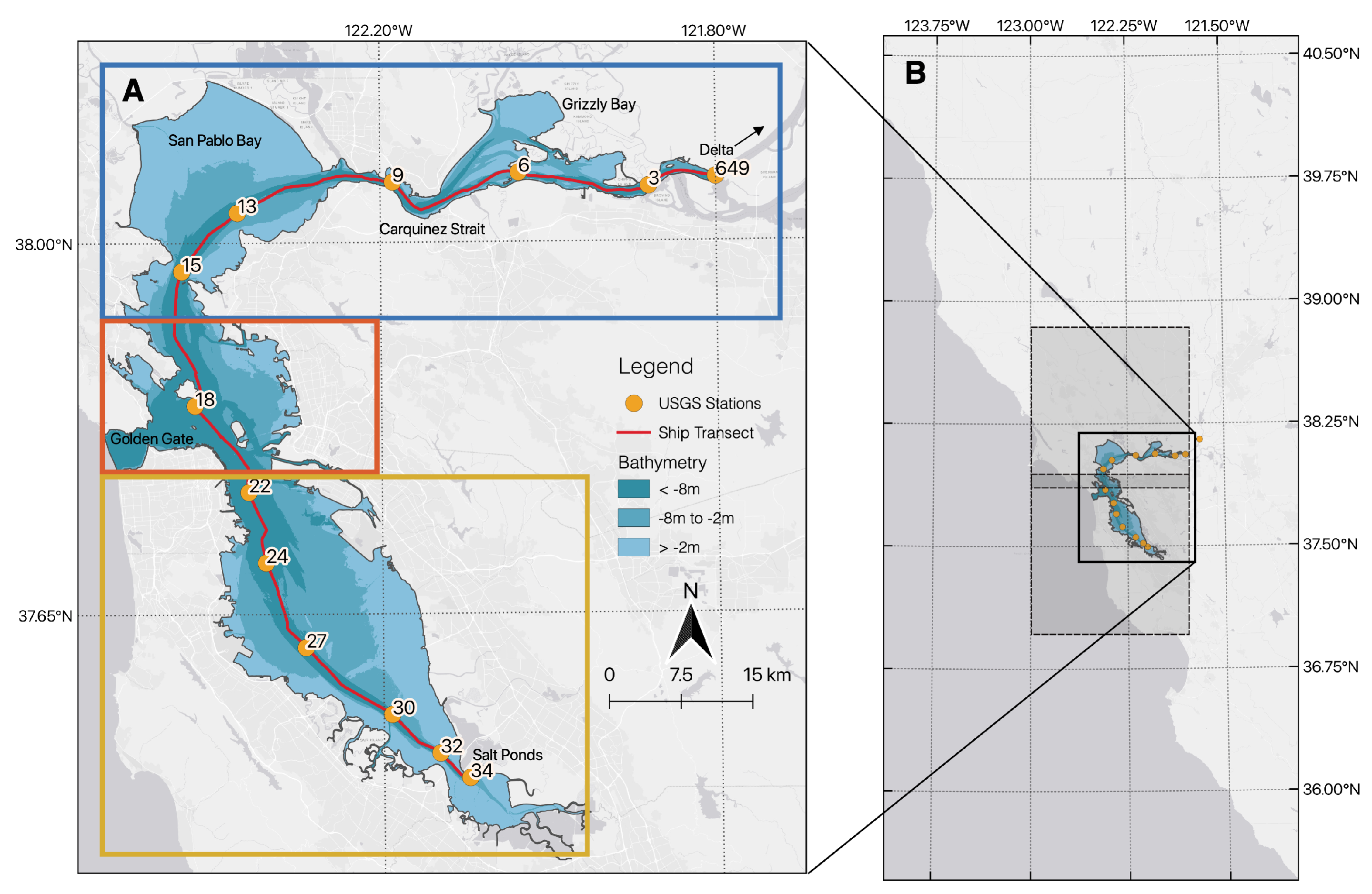
2.1. Study Area

SF Bay can be simplified into three main regions: the North Bay, Central Bay, and South Bay (Figure 1). These regions can be approximately defined by the location of bridges crossing the Bay: North Bay is the region of the Bay north of the Richmond Bridge, Central Bay is the region between the Richmond and Bay Bridges, and South Bay is the region south of the Bay Bridge. These regions each experience different physical processes driving water movement and spatial variability.The bay overall is a shallow wetland system, with most of the bay less than 3 m deep (Figure 1). The exception to this is a dredged shipping channel which runs through the middle of SF Bay from North to South. This shipping channel is the deepest part of SF Bay (depths greater than 10 m) and is dredged regularly to facilitate the movement of ship traffic. This stark difference in bathymetry and higher flow velocities in the shipping channel [14] make it distinctive from the rest of the bay.
The full SF Bay is connected to two major water bodies: the San Francisco Bay Delta to the northeast, and the Pacific Ocean to the west. The San Francisco Bay Delta feeds into east North Bay and is where the Sacramento and San Joaquin rivers combine. Inflow from the Delta accounts for 90% of the total freshwater inflow to the Bay. North Bay is therefore characterized by a strong salinity gradient, and this inflow of river water is the primary control on bay-wide salinity [1]. The Delta inflow is also the primary source of suspended sediments, nutrients, and freshwater phytoplankton to the estuarine system [23]. The remaining 10% of inflow to the Bay comes from runoff and other point sources.
Flow out of SF Bay is primarily controlled by the amount of freshwater inflow from the Delta [23]. The Bay drains into the Pacific Ocean through the Golden Gate (Figure 1), which exerts strong tidal influence on horizontal mixing within SF Bay moving water back and forth over 10’s of km. The combination of inflow from the Delta, tidal mixing from the Pacific, varied bathymetry, and wind-driven mixing creates a highly dynamic system. Each type of physical forcing has different levels of influence on North, Central, and South Bay: for example, the strong salinity gradient set up by Delta flow in North Bay creates a very different environment than South Bay. Water retention time in South Bay is on the order of 3–5 months, while in North Bay water moves through as quickly as 2 weeks [23].

2.2. Data Overview

To examine how remote sensing methods can supplement existing in-water monitoring methods, we collected four types of data in collaboration with the USGS Water Quality Monitoring Program. We used in situ SPM grab sample measurements and continuous turbidity flowthrough data taken by the USGS in collaboration with UCSC as part of their standard monitoring procedure; continuous radiometric data taken from the bow of the USGS research vessel, the R/V Peterson; and 10 m satellite imagery from the MultiSpectral Imager (MSI) onboard the European Space Agency’s Sentinel-2 satellite. In sum, we used discrete SPM grab samples, continuous flowthrough and shipboard radiometry taken along a transect, and spatially complete satellite imagery covering the full bay.
The ground-based data used in this study were collected on 25 April, 4 June, and 23 October 2019 onboard the R/V Peterson. Each cruise began at approximately 6:00 a.m. local time (PDT) from Redwood City harbor and ended between 3 and 5:00 p.m. in Antioch (Figure 1). Sentinel-2 imagery was always acquired at 11:30 a.m. PDT. Sentinel-2 overpasses occurred on both the April and June dates. No Sentinel overpasses occurred on 23 October, so instead we used imagery that was collected on 22 October.

2.3. USGS In-Water Data

Water quality measurements including SPM concentration (mg/L) were collected at regular point stations (Figure 1) at 2 m depth, according to USGS standard operating procedures. Quality controlled data from the USGS are available for public use (sfbay.wr.usgs.gov, accessed 21 January 2020).
Continuous underway measurements of turbidity were collected every 5 s at 2 m depth throughout each cruise using a Turner Designs Self-Contained Underwater Fluorescence Apparatus (SCUFA). These underway flowthrough data were validated following the standard operating procedure of the USGS San Francisco Bay Water Quality Monitoring program [12]. Briefly: data were filtered to remove bubble noise in the system. Flowthrough data taken while the ship was sampling at designated stations (Figure 1) were averaged and compared to corresponding discrete samples using linear regression. If the regression line had an R 2 > 0.7, the relationship was accepted and used to convert all the filtered flowthrough data to SPM units. If the R 2 was less than 0.7, the data was geographically split into groups of at least three points. A new regression was fit for each group and used to convert flowthrough data contained in each group to SPM.

2.4. Shipboard Radiometry Data

In addition to the regular USGS data, a HOBI Labs HydroRad-3 (HydroRad) hyperspectral radiometer was mounted at the ship’s bow and set to record continuously throughout each cruise. Discrete hyperspectral measurements from an Analytical Spectral Device (ASD) FieldSpec HandHeld 2 Spectroradiometer were also taken to corroborate HydroRad data at locations corresponding to simultaneous water quality measurements. Prior to being deployed, the data quality and signal to noise ratio of the HydroRad was checked against the ASD in stable conditions. Onboard the R/V Peterson, the HydroRad recorded continuous radiometry measurements of downwelling irradiance ( E d ), sky radiance ( L s k y ), and total radiance from the water ( L T ). The HydroRad’s three sensors were fixed 2 m above the main deck on the ship bow. Care was taken throughout the cruise to keep sensors pointing 100 –130 average solar zenith angle. L T was fixed 40 down from horizontal, L d was fixed 40 up from horizontal, and E d was fixed vertically.
HydroRad data collected before station 24 were removed to eliminate data collected in low-light conditions (i.e., solar elevation below 30 ). The remaining data were processed following [24]. Remote sensing reflectance ( R r s ) was calculated from the HydroRad data using the equation:
R r s   =   L T ( λ )     ρ L s k y ( λ ) E d ( λ )
where λ is wavelength, and ρ s k y = 0.1 to correct for skylight reflectance off the water surface [24]. Data were inspected for quality control and manually compared to ASD measurements. Flat spectra, spectra with negative values, and oversaturated spectra were removed, and high frequency noise (attributed to glint) was removed from the remaining data using a running mean with a smoothing value of 2.
SPM was calculated from HydroRad R r s along each cruise track using the single-band algorithm developed by [19], following the successful use of the algorithm in SF Bay by [8]. This algorithm uses a single channel to determine SPM based on spectral brightness, and then uses an empirically derived set of coefficients to calculate SPM. We chose to synthesize a band centered at 700 nm by averaging all hyperspectral channels within an 8 nm window to mitigate noise effects; 700 nm was deemed appropriate based on the recommendations in [19], preliminary tests, and an observed increase in sensor noise above 700 nm. Retrieved SPM values from data taken at stations were compared to validated flowthrough SPM for each cruise (Figure 2).

2.5. Satellite Image Processing

In addition to shipboard radiometry, we tested the applicability of retrieving SPM with Sentinel-2 using existing algorithms. Because our goal was to test the applicability of existing tools to SF Bay in order to identify the best practice for repeated monitoring, no additional calibration was performed on any of the algorithms. To examine SPM outside the shipping channel, we use imagery from Sentinel-2 overpasses on 25 April, 4 June, and 22 October 2019. Concurrent USGS cruises with radiometry occurred on 25 April and 4 June. No ground data was collected on 22 October, but data were available from a cruise on 23 October. A 1 day difference is outside the temporal window for comparison in SF Bay [8]. Consequently, direct comparisons between ground and satellite data are only made for April and June, and the October data are simply used as a qualitative check.
For each date, two images of SF Bay were acquired sequentially at approximately 11:30 am PDT. Sentinel-2 granule 10SEH covers the northern half of SF Bay, and granule 10SEG covers the southern half. No concurrent imagery was available for the Delta region (granule 10SFH) encompassing station 657 for any of our dates because it is imaged on a different cycle. Imagery was downloaded from the ESA open-access data portal (scihub.copernicus.eu) in two different versions; one set of Level 1C top-of-atmosphere (TOA) reflectance, and a second set processed to the ESA’s atmospherically corrected Level 2A bottom-of-atmosphere (BOA) reflectance. Images were mosaicked using the ESA’s open-source imaging processing software, SNAP, to create full Level 2A image and a full Level 1C image for each date.
We tested three retrieval methods for mapping SPM using the Sentinel-2 imagery. We first tested the single-band ([19]) SPM algorithm applied to the Level 2A surface reflectance. Per the requirements of the algorithm, we selected band 4 (665 nm) which is the band farthest into the red that has 10 nm spatial resolution.
Due to known issues with the Level 2A atmospheric correction over coastal waters, we also tested the Case 2 Regional CoastColour (CR2CC) processor in SNAP with Level 1C TOA imagery. The CR2CC processor was developed specifically for remote sensing of water, and simultaneously atmospherically corrects imagery and retrieves optically relevant water quality variables (including SPM concentration). C2RCC uses a set of neural networks to match observed conditions with a library of radiative transfer simulations representative of different water types [20]. It has been specifically developed to work with certain satellite sensors, and therefore was not transferable to the shipboard HydroRad dataset.
All atmospherically corrected reflectance products are compared in Figure 3. Surface reflectance from Sentinel-2 was converted from surface reflectance to R r s by dividing by pi to compare with HydroRad R r s . Processing steps for all SPM retrievals are documented in Table 1.
To evaluate the validity of each atmospherically corrected product, we compared both (the reflectance from Sentinel-2 processed with C2RCC and the reflectance from the standard Level 2A Sentinel-2 product) to reflectance measured by the HydroRad at the surface (Figure 3). We also compared the satellite SPM retrievals with the HydroRad SPM retrievals and the in-water SPM measurements. In total, we compared five continuous SPM transects (Figure 4A,C), including: (1) the USGS in-water flowthrough data, (2) the SPM retrieved from the HydroRad using the single-band [19] algorithm, (3) SPM retrieved using the single-band [19] algorithm and the standard Level 2A Sentinel reflectance product, (4) SPM retrieved using the single-band [19] algorithm and the C2RCC Sentinel reflectance product, and (5) SPM retrieved using just C2RCC. For each retrieval strategy, we calculated the absolute error as compared to the flowthrough data to evaluate overall accuracy (Figure 4B,D).

2.6. Spatial Variability Analysis

We examine spatial variability using the SPM distribution maps created from Sentinel-2 imagery using the Ground Sampling Distance ( G S D ) vs. Coefficient of Variance ( C V ¯ ) method outlined by [21] and modified slightly in this study. This analysis defines the amount of spatial variability at different scales. The method is similar to a semi-variogram or spatial autocorrelation, but we chose this method over others because it is mathematically similar to an inverted Signal to Noise Ratio or uncertainty metric. This allows us to think of the C V ¯ as a measure of how representative a single sample is for an area. As larger and larger areas are considered, the variability increases rapidly at small scales first and then more slowly at larger scales, following a logarithmic relationship.
The amount of spatial variability is calculated as a function of increasing distance or area (Ground Sampling Distance, G S D ). Spatial variability was quantified as the Coefficient of Variance ( C V ¯ , [21]), defined as
C V ¯   =   1 n i   =   1 n ( 1   +   1 4 k ) σ i x ¯ i
where n is the number of segments the dataset is broken into, k is the number of data points in each segment, x ¯ i is the within-segment mean, and σ i is the within-segment bias-corrected standard deviation. The C V ¯ is essentially a measure of how representative a single measurement is for an area defined by G S D .
The rate at which variability is gained with distance can be quantified as d C V ¯ / d G S D . We modeled the relationships between C V ¯ and G S D for each dataset using a logarithmic function [21]. The transition point where this rate changes ( G S D T ) represents the sampling distance at which variability begins to increase more slowly. Moses et al. used two different methods for finding the transition G S D : the first was the find a log-log intersect, and the second was to identify the G S D where slopes reached the 66th percentile. Our data did not display any clear log-log intersect, and the 66th percentile method was arbitrary and did not transfer to our study. Instead, we defined the G S D T as the G S D where d C V ¯ / d G S D = 1 × 10⁻⁴, i.e., where the slope transitioned through 1% C V ¯ per 100 m. This gives us a fixed metric to compare across our datasets and represents a clear transition point in d C V ¯ / d G S D .
We conducted three distinct spatial variability comparisons. First, we calculated the C V ¯ / G S D relationship for the full Bay on each date to examine how variability changed between months. Second, we compared those full Bay relationships with variability in just the shipping channel. This was done by extracting just SPM values along the USGS cruise transect and repeating the variability analysis using just the data within the shipping channel. Third, we examined the variability in different regions of the Bay by repeating the analysis for the North, Central, and South Bay regions.

2.7. Environmental Data

We obtained Delta flow data from the California Natural Resources Agency’s Dayflow dataset, which is an algorithm used for tracking historical mean daily flows into SF Bay from the Delta (data.cnra.ca.gov, accessed 21 May 2021). Information on tidal phase and state is from NOAA’s Tides and Currents Water Level product for SF Bay (tidesandcurrents.noaa.gov, accessed 21 May 2021). Wind data were taken in situ at each station as part of the radiometry data collection protocol. At the time of each satellite overpass, wind was measured at 7.7 m/s, 0.5 m/s, and 1.3 m/s at USGS station 13, which is where the R/V Peterson was sampling at the time.
Tidal conditions on each date were as follows. In April, SF Bay was transitioning from spring to neap tide conditions, and imagery was taken at a peak high tide of 1.6 m. The June image was taken at the height of spring tide, during a falling tide at 0.6 m with the tide going out at time of satellite overpass. In October conditions were switching from spring to neap tide, and it was a falling tide at 0.6 m with the tide going out at the time of the satellite overpass. All imagery was taken at 11:30 a.m. PDT.
Delta flow on each date followed seasonal patterns. The inflow from the Delta was similar for April and June (rainy season), then much lower in October (dry season). Delta inflow in April was 68,464 cfs (cubic feet per second) and in June was 66,005 cfs. The April cruise occurred following a large peak in flow, and the June cruise occurred at the height of a local peak in delta flow. In October, Delta inflow dropped by a factor of four to 15,845 cfs.

3. Results

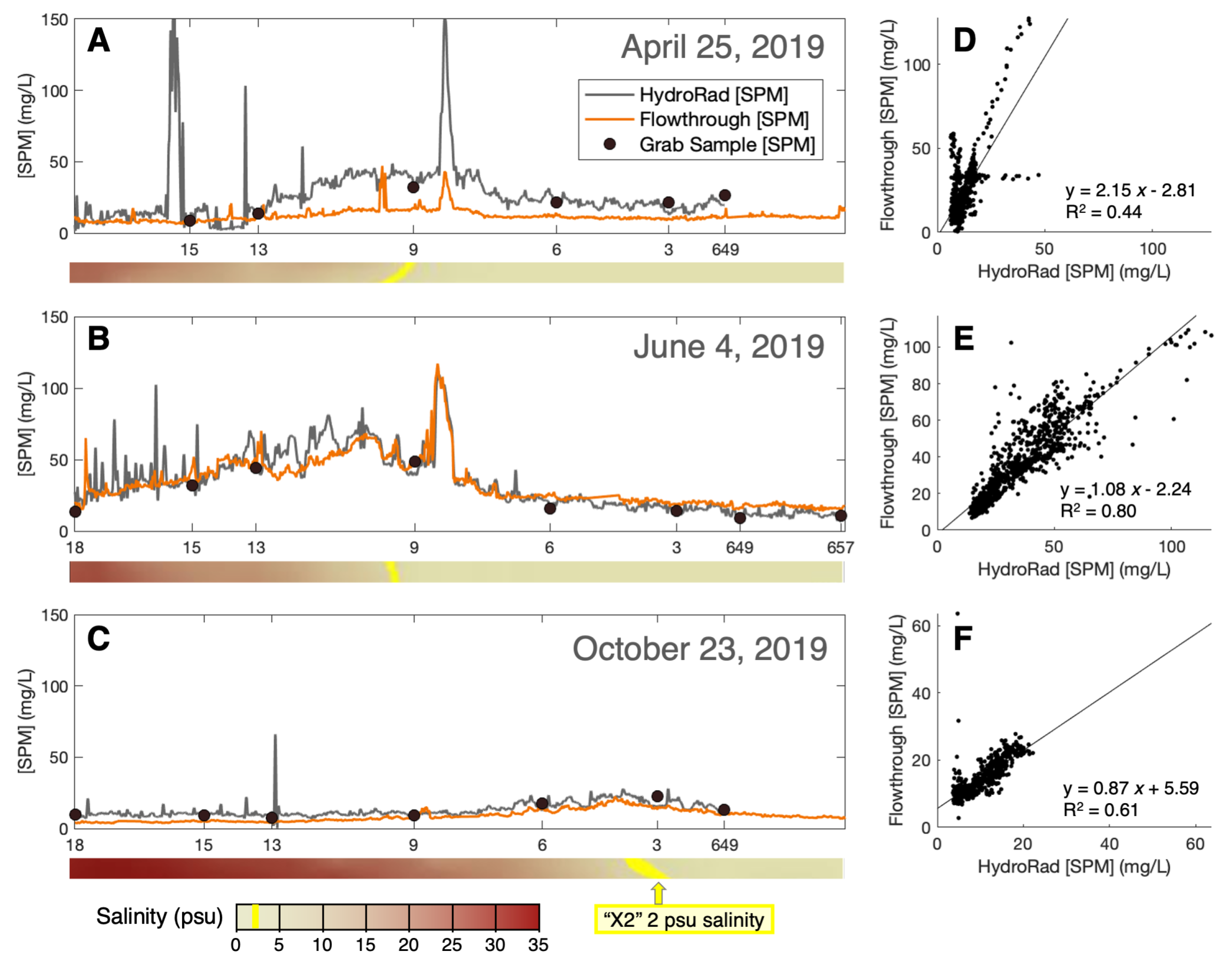
3.1. Shipboard Radiometry and Flowthrough Comparison

The relationship between retrieved SPM from the HydroRad and in situ SPM from the flowthrough system was correlated ( R 2 ⩾ 0.49) on each cruise. This correlation stayed near a 1:1 relationship but differed from cruise to cruise. HydroRad SPM appears to underestimate the flowthrough SPM (slope = 2.15) in April but were more aligned in June and October (slopes of 1.08 and 0.87, respectively) Figure 2.
The full transects of HydroRad SPM, flowthrough SPM, and in situ grab samples are compared in Figure 2. The average distance of grab sample measurements is 8 km, and the average distance between HydroRad measurements was 95.8 m, excluding data gaps and repeats taken when the boat was paused at stations. Notably, a SPM maximum can be identified in all datasets and corresponds with the location and slope of the salinity gradient Figure 2. In April the region of the SPM maximum and salinity transition point are mid-way in the Carquinez Strait near station 9; in June, both features are present just west of station 9; and in October, the transition point moves eastward into the Sacramento River near station 3.
Smaller notable features also occur in the transects. A significant peak occurs near station 9 for all dates, although the exact location of the peak shifts slightly Figure 2. This persistent turbidity feature in the Carquinez straight is not captured by the grab sample stations. The magnitude of this feature changes, from approximately 40 mg/L in April, up to 120 mg/L in June, and down to 15 mg/L in October.

3.2. Satellite Retrievals

Figure 3 shows the comparison of different atmospherically corrected Sentinel-2 products with corresponding surface-level HydroRad spectra. All data were normalized to 740 nm. The C2RCC R r s product was visibly a better match with the HydroRad spectra than the standard Level 2A reflectance product, which consistently over-estimated the overall brightness of the signal.
Retrieved SPM products from atmospherically corrected Sentinel-2 data are compared in Figure 4 to the HydroRad SPM product and the in-water flowthrough data. For each retrieval strategy, the absolute error as compared to the flowthrough data was calculated (Figure 4C,D). The standard Level 2A reflectance product with the Nechad algorithm had the highest error. The C2RCC correction had lower error with both the Nechad algorithm and the C2RCC algorithm: in April, the Nechad algorithm outperformed the C2RCC algorithm, but in June the C2RCC algorithm had lower error. Because of the observed difference between the HydroRad and the flowthrough data in April, and the hypothesized stratification confounding results on that date, we elected to use the Sentinel-2 retrieval that had the lowest error on the June date: the C2RCC atmospheric correction and C2RCC SPM retrievals.

3.3. Satellite SPM Results

C2RCC was used to generate maps of SPM on 25 April, 4 June, and 22 October (Figure 5). General statistics for each date are presented in Table 2. April and June displayed high concentrations of SPM, with mean values of 46.25 mg/L and 47.78 mg/L, respectively. In contrast, October had a mean value of 9.06 mg/L. The range for each date was 149.58 mg/L, 148.83 mg/L, and 46.21 mg/L for April, June, and October, respectively. Lower South Bay and upper San Pablo Bay consistently had the highest SPM. Central Bay had the lowest SPM values—in June and October, the lowest SPM values are at the Golden Gate; but in April, that section of SF Bay was blocked by clouds. Other prevalent spatial patterns included low SPM values in the northern section of the shipping channel in April and June, and consistent filamented structure in the middle of South Bay.
Differences in SPM and spatial structure on each date include the widening of the low-SPM area in the shipping channel through San Pablo Bay in the June image compared to the April image. Changes in SPM along the Delta to North Bay gradient through Grizzly Bay occur as the system shifts from high Delta flow conditions (April and June) low Delta flow (October). Closer inspection of the Carquinez straight and Grizzly Bay also elucidate the structure of the Carquinez straight feature observed in the transect data (Figure 3): a filament of high SPM runs along the northwestern shore of Grizzly Bay and intrudes into the shipping channel cruise track (Figure 5). This pattern is most pronounced in the June image. The high-SPM filament moves from the shore in April/June to the middle of the channel in October.

3.4. Spatial Variability Analysis

To quantify how much variability exists at different spatial scales in SF Bay, we calculated the relationship between spatial scales defined by the G S D and variability defined by C V ¯ . Results are displayed in Figure 6. For all datasets, the relationship between G S D and C V ¯ followed the logarithmic relationship described by [21]. We considered the modeled C V ¯ as a measure of how representative a single measurement is of a surrounding area of size G S D . The rate of change, d C V ¯ / d G S D , was consistently positive for all datasets. We specifically address two metrics: the Transition G S D ( G S D T ); and the C V ¯ at a G S D of 5 km ( C V ¯ 5 km). The G S D T is the inflection point where d C V ¯ / d G S D switches from rapidly increasing to slowly increasing and indicates the scale ( G S D ) at which variability begins to level off. The C V ¯ 5 km is the C V ¯ at the 5 km scale, which is the approximate scale of USGS point sampling in the Bay.

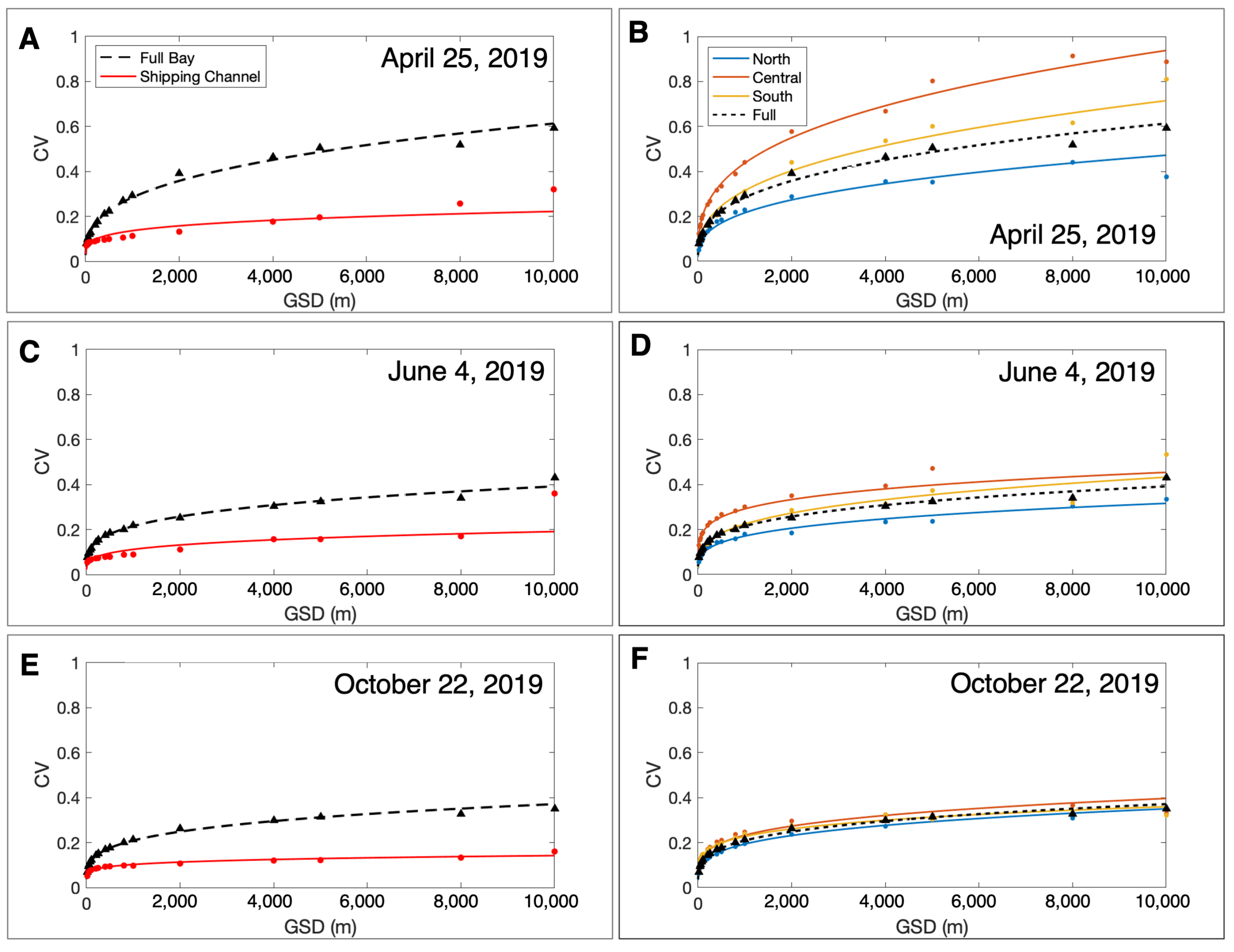
3.4.1. Comparison between Dates

April exhibited the most variability across all scales ( G S D s) for all the dates sampled. Specifically, the C V ¯ 5 km decreased by 0.2 from April to June and October (full area C V ¯ 5 km of 0.51, 0.32, 0.32). June and October had much more similar variability with C V ¯ 5 km of 0.32 for both dates (Figure 6A,C,E). This is also reflected in the G S D T metric for each date: April, June, and October, respectively, had G S D T values of 921 m, 461 m, and 421 m, indicating much more heterogeneous conditions in April than the other two months.
This pattern of heterogeneity was not reflected in the shipping channel-only analysis (Figure 6A,C,E). Although April still had the highest variability, June and October had different levels of variability within the shipping channel. C V ¯ 5 km within the shipping channel was 0.2, 0.16, and 0.12 for April, June, and October, respectively.
Comparing the shipping channel to the full area of SF Bay (Figure 6A,C,E), we found that there is approximately twice the amount of variability in the full area than just the shipping channel transect. This approximate doubling of variability is consistent across different regions and dates but does change with scale. At smaller scales (i.e., 100 m), the ratio of area variability to transect variability is approximately 1.5; but above a 1 km scale, the ratio is approximately 2.

3.4.2. Regional Comparison

For all dates, Central Bay had the highest C V ¯ at all G S D s, followed by South Bay, then North Bay (Figure 6B,D,F). Specifically considering the average across all dates, North, Central, and South Bay had an average C V ¯ 5 km of 0.3, 0.53, and 0.43, respectively. At a smaller scale of G S D = 100 m, North, Central, and South Bay each had an average C V ¯ of 0.1, 0.18, 0.13 compared to an average full bay C V ¯ of 12%. The d C V ¯ / d G S D for South Bay was lower than other regions of SF Bay (illustrated by slower increase in C V ¯ / G S D relationship, Figure 6B,D,F), implying less small-scale variability. Variability conditions in Central and South Bay were also more inconsistent than North Bay: between all dates at G S D = 10 km, the C V ¯ of Central Bay ranged 0.32–0.89, South Bay ranged is 32–81%, and North Bay ranged 0.33–0.37. This indicates that North Bay has the most consistent C V ¯ / G S D relationship and spatial structure of the three regions.
The G S D T values for each region (Table 3) also indicate that North Bay has less spatial variability than Central and South. The G S D T represents the scale at which spatial patterns begin to become more homogeneous and indicates dominant physical mixing processes. A larger G S D T corresponds to more spatial variability in the environment, and a lower G S D T corresponds to less spatial variability. The average G S D T for each region was 451 m, 894 m, and 698 m for North, Central, and South Bays, respectively. A similar but pattern is represented in the transect G S D T values of 118 m, 138 m, and 174 m for North, Central, and South Bays. Notably, the G S D T of the shipping channel transects are lower than the G S D T of the full areas. Also, the transect G S D T s of regions do not consistently correspond to the area G S D T s. For example, in June, the relative patterns of the transect and area G S D T s are the same: South Bay has the highest G S D T for both the transect and areas, and North Bay has the lowest for both. However, in October, the relative patterns of the transect and area G S D T s are different: the Central Bay transect G S D T is smaller than North or South Bay, but the Central Bay area G S D T is larger than the other two regions.

4. Discussion

4.1. Comparison of Datasets

Shipboard radiometry retrievals matched in situ measurements better than any of the retrievals from the Sentinel-2 data, for both April and June (Figure 4). Changes in the relationship between HydroRad retrieved SPM and validated flowthrough SPM occurred on each date, notably the April matchup relationship had a slope of 2.15 rather than 1 (Figure 2). The discrepancy in the April data could potentially be due to stratification occurring between the in situ grab samples at 2 m depth and the surface SPM concentration retrieved by the shipboard HydroRad. Intensified stratification from high Delta inflow and switching tides could have contributed to the inconsistency between surface radiometry data and flowthrough data at depth. The shipboard radiometry has comparable data to a flowthrough system and is more convenient in that it could easily be set up on small boats or commercial boats already moving around SF Bay. This concept could be highly relevant in SF Bay if scientists partner with commercial vessels.
Retrievals with Sentinel-2 data were able to capture spatial patterns of SPM, with varying success (Figure 4). Using C2RCC to both atmospherically correct and retrieve SPM had relatively low error and was easy to implement using SNAP. C2RCC corrected reflectance matched best with shipboard radiometry, whereas the standard Level-2A reflectance product had much higher brightness across channels (Figure 3). Although C2RCC retrievals did seem to consistently overestimate SPM concentration in April and June, overall it tracked in situ flowthrough data well (Figure 4). The authors of [18] also tested a suite of methods for SPM retrieval at the mouth of the Mzymta River, and also observed a high correlation between C2RCC retrievals and in situ measurements when SPM concentrations were above 20–25 mg/L. In our study (and broadly in SF Bay), SPM concentration was often above this threshold, especially in April and June. However, in October, SPM concentration dropped below the threshold. Since we had no directly corresponding ground data for October, we were unable to confirm the validity of the C2RCC method in SF Bay at lower (<20–25 mg/L) concentrations. More data are required to address this concern and should be noted for future studies.
All sources of continuous shipboard and satellite data captured more variability and SPM features than point sampling. Additional features are visible in the shipboard radiometry flowthrough, and satellite datasets—notably including a peak just after station 9, corresponding to a known gravity circulation feature coming out of Grizzly Bay [7]. At a larger scale, the datasets capture a regional maximum in SPM that corresponds to the location of the X2 salinity marker (Figure 2 and Figure 4). This matches what has been described in previous work as the North Bay Estuary Turbidity Maximum (ETM) zone [7] which serves as an important habitat indicator for estuarine species and marks the transition from fresh to saltwater. X2 tracks the location of the ETM, which in turn is associated with a region of salinity preferred by estuarine species like Delta Smelt [7], and marks the approximate region of transition between marine and freshwater phytoplankton [25,26]. The location of the ETM is dictated by flooding, which controls SPM supply [2,5]. Wind re-suspends SPM, and tides create oscillations in ETM location, which may explain the land- and seaward shifts in the ETM observed in our data. Future work connecting the location of the ETM, spatial variability of SF Bay, and environmental conditions could help inform seasonal requirements for monitoring programs.
The general trade-offs between the methods for monitoring SPM presented in this study are clear: as spatial coverage increases, overall accuracy is lost. This is a function of the additional sources of error that confound SPM with remote sensing (i.e., the accuracy of the atmospheric correction and retrieval algorithm used). It is important for stakeholders to consider what level of accuracy is required to answer various questions and address various issues. Satellite imagery provides a broad and resolved view of SPM distribution; in contrast, point measurements provide certainty that is virtually irreplaceable. As remote sensing technology and retrieval algorithms continue to improve, the trade-off between accuracy and spatial coverage is becoming easier to reconcile. A major focus now is handling and utilizing the shear amount of data and information remote sensing can provide.
While we primarily use shipboard radiometry to connect in situ data to satellite data, it should be noted that shipboard radiometry is a valuable data source in its own right. Shipboard radiometry systems like the HydroRad used in our study provide hyperspectral data. We did not explicitly use the sensor’s hyperspectral capacity in this study, but calls for increasing the collection of hyperspectral data in coastal ocean systems are increasingly widespread [27,28]. Consistent hyperspectral data sources could expand biological monitoring in SF Bay and improve our understanding of chlorophyll spatial variability and phytoplankton functional types [27,29]. At minimum, collecting shipboard radiometry provides hyperspectral data with no atmospheric influence at 100 m resolution that could be used for calibration and validation of future hyperspectral sensors like the upcoming Phytoplankton, Aerosol, Cloud, Ecosystem (PACE) and proposed Surface Biology Geology (SBG) missions. Although this study largely overlooks the advantages of having a hyperspectral data source, other studies have demonstrated the potential for retrieving multiple water quality variables from hyperspectral data [9,30]. Empirical retrieval algorithms created using hyperspectral data in Estuary systems are highly accurate when created with sufficient data [31], so having consistent hyperspectral data collection with a shipboard system could facilitate improved retrievals and additional variables to SPM. Using hyperspectral data could help retrieve a suite of water quality variables, which would be particularly helpful for ongoing monitoring of algae and pollutants in SF Bay.

4.2. Spatial Variability

Differences between Dates

Changes in the C V ¯ / G S D relationships between dates corresponded to changes in environmental conditions. Seasonal changes in Delta flow, tidal state, and wind speed in combination with different tidal phase are well known to influence SPM variability [2,6,32,33], and influence G S D T and C V ¯ s across scales.
The high SPM concentrations in April and June corresponded to the high Delta inflow as compared to October, and to different tidal phases. Delta flow has been directly related to the overall SPM concentration in SF Bay [2,33]. The authors of [2] documented SPM plumes from large freshwater flows from the Delta in their analysis of AVHRR-derived SPM. It therefore makes sense that April and June had higher SPM at times of relatively high Delta outflow (68,464 and 66,005 cfs, respectively), compared to the low SPM in October corresponding to low (15,000 cfs) Delta outflow. Tidal phase is also linked to high and low SPM concentration: spring tides correspond to high SPM, and neap tides correspond to low SPM [7]. 25 April occurred just before a spring tide, 4 June occurred at the height of a strong spring tide, and 23 October was the beginning of a neap tide.
Daily changes in tidal height also affect overall SPM concentration, but also affect SPM distribution [2,33], which may explain the high variability in April as compared to June and October. The April image was taken during a high tide of 1.6 m, while both the June and October images were taken at a tide height of 0.55 m. Changes in tidal height between images account for significant differences in spatial distribution of turbidity and SPM [9], and could explain the consistently higher C V ¯ s observed in April (Figure 6), especially since variability was particularly high in Central Bay which is the most affected by ocean tides.
Changes in wind stress have been shown to affect SPM distribution by controlling re-suspension [6], especially in shallow areas of SF Bay [2]. While we did see higher SPM concentrations in shallow areas of SF Bay on the date with high wind speeds (April, Figure 5, Table 2), this is highly speculative. Wind direction is also important [6] and was not recorded, so more data would need to be examined to draw specific conclusions about the effects of wind on the dates we examined.
We only consider three dates from 2019, but conditions in SF Bay can change dramatically year to year: for example, Delta flow throughout 2020 was much more similar to flow in October 2019 than April or June 2019. Future research should examine spatial structure and variability over a longer time period, during more tidal states, Delta flow conditions and more extensive wind data. Coupling high-resolution SPM remote sensing and physical models of SF Bay (i.e., [6]) could elucidate the relationships between SPM variability and environmental conditions. We recommend using a Principal Component Analysis or similar method to identify regions and times of high and low SPM variability, which could provide valuable information for in-water sampling design.

4.3. Differences between Regions

Central Bay consistently had the highest variability, followed by South Bay and then North Bay (Figure 6B,D,F), which we suggest is linked to its proximity to the ocean and therefore the influence of tides. Because we did not normalize our C V ¯ / G S D relationships, and modified the calculation of G S D T , we cannot quantitatively compare our results to [21]. However, [21] observed a decrease in variability in areas with less physical mixing (i.e., offshore), which matches what we observed (i.e., North and South Bay have less physical mixing and less variability than Central Bay).
The results from the C V ¯ / G S D relationships between regions show that North Bay has consistently less spatial variability than Central and South Bay (Figure 6B,D,F), represented by a lower G S D T for North Bay compared to the other regions. This is initially counter-intuitive because North Bay is often thought of as highly dynamic compared to South Bay: water residence times in North Bay are approximately 2 weeks, compared to South Bay water residence times of approximately 3–5 months [1]. However, this relatively low heterogeneity matches what is seen in the satellite imagery. For example, if we consider April as a case example: the G S D T of North Bay is 621 m compared to 1.7 km and 1.2 km for Central and South Bay, respectively. Looking at the SPM map for that day, we see that the main source of variation in North Bay is the distinctive shipping channel. However, most of the North Bay region falls within the smaller range of SPM = 60–145 mg/L, whereas both Central and South Bay have a larger range of SPM = 30–145 mg/L. Central and South Bay also don’t have just one single distinctive feature the way North Bay does—instead, there is more widespread heterogeneity across the full area of each region, driving up the G S D T . The strong influence of Delta flow in North Bay results in dynamic movement, but steady spatial structure. In contrast, Central and South Bay water movement is less controlled by Delta flow and instead primarily correlated to tidal phase [3,34], which sets up less consistent structure and results in higher spatial variability. South Bay C V ¯ / G S D has a lower slope than other regions, which is especially apparent in the transect data.

4.4. Differences between the Shipping Channel and Full Bay

In the full bay vs. shipping channel analysis, the variability of the entire bay was consistently higher than the variability observed in the shipping channel (Figure 6A,C,E). Results show there is twice as much variability when considering the full bay compared to just the shipping channel transect. Our results suggest that data taken just within the shipping channel will underestimate the variability that exists in the full bay. This can be attributed to two things: first, the shipping channel is a distinctive region from the rest of the bay: it is potentially more homogeneous than the rest of SF Bay because it is consistently deeper (Figure 1) and experiences less wind-driven re-suspension of SPM [6]. Second, the data in the shipping channel were extracted along a transect and are therefore one dimensional while the full area dataset is two dimensional. This is important because variability in SF Bay is not isotropic. Previous studies that have looked at spatial variability in the cross-channel direction [2,9,32] confirm that spatial variability in SF Bay is anisotropic, with more heterogeneity in cross-channel datasets than within-channel datasets.
Our C V ¯ / G S D analysis assumes isotropic conditions in the Bay and overlooks the longitudinal anisotropy that exists because of the shipping channel’s distinctiveness. Anisotropy could be examined more effectively using a different spatial variability analysis, such as a semi-variogram method that considers the North-South anisotropy introduced by the shipping channel. This can be done by including the direction of strongest correlation and the anisotropy ratio. Despite its limitations, the C V ¯ / G S D analysis does effectively illustrate the potential issues with monitoring the Bay only along the shipping channel transect: the channel is physically distinctive and sometimes less heterogeneous than the full bay. Integrating satellite image processing with current monitoring methods would not only provide spatially resolved information, but also provides context on cross-channel variability that is not regularly tracked.

4.5. Implications for Monitoring

Monitoring at different resolutions in different parts of SF Bay could be informed by this analysis. Like results from other coastal areas [21], high variability at sub-kilometer scales is observed in SF Bay. In a broad analysis of coastal oceans, the authors of [35] cautioned that for a 30–1000 m area, a single in situ point measurement can have errors up to 18%. In this study, we show that point measurements at 30–1000 m could have much higher error (20–40%) depending on the conditions at any given time. The highly dynamic nature of the SF Bay estuary system also means that there is essentially no point at which spatial structure becomes uniform. Therefore, monitoring decisions about sampling resolution and strategy should be made on a case-by-case basis, based on what processes are being examined and when and where the monitoring is occurring. This is certainly true for SF Bay, and is likely broadly applicable to other estuaries and highly dynamic systems.
Several recommendations emerge from this study. First and foremost, we emphasize the lack of variability captured in the shipping channel. Spatial variability in SF Bay is not isotropic, and the spatial structure of the shipping channel is not necessarily representative of the spatial variability in the rest of SF Bay. Considering data taken at dispersed stations throughout the area of SF Bay is important for any research looking to assess water quality changes or changes in SF Bay conditions. Reliance on point measurements or transect data taken solely in the shipping channel increases the likelihood of missing important outflow events or seeing peaks that are part of a larger feature or small filament.
Similarly, monitoring in different areas of SF Bay should consider the scales at which processes occur, and consider how much inherent uncertainty is incorporated with monitoring at different resolutions. For example, using the C V ¯ / G S D relationship established for April, Central Bay has a C V ¯ of 0.1 at 20 m resolution, whereas the equivalent C V ¯ in North Bay is much higher at 190 m resolution. Accordingly, monitoring in Central Bay must occur at higher spatial resolution than North Bay in order to capture the same level of variability. While this highlights the advantages of high-resolution datasets—like that of Sentinel-2—and provides information for in-water monitoring strategies, our study does not inform on how sampling points could be optimally distributed. We recommend future studies build off this work by using satellite imagery to identify unique and distinct features at different times of year, different tidal states and different Delta conditions.

5. Conclusions

Monitoring stations placed 5 km apart diagnose general water quality and keep track of changes in overall Bay conditions but miss multiple features at smaller spatial scales and do not capture the full variability of SF Bay. Remote sensing data from satellites and from ships can supplement existing monitoring programs by providing increased resolution and broader spatial coverage. We demonstrate this by comparing in situ measurements with SPM retrievals from a ship-based radiometery system and Sentinel-2 imagery collected on three dates in 2019. Retrievals from the ship-based radiometry data were more accurate than retrievals from the satellite data, but using the C2RCC processor for both atmospheric correction and SPM estimation we were able to map spatial patterns with Sentinel-2. Images of SPM spatial distributions were used to understand spatial variability in different areas of SF Bay in April, June, and October—each of which was associated with different physical environmental conditions. We found that Central Bay consistently has the most spatial variability across all scales, while North Bay has the lowest heterogeneity. In addition, we show variability in the main shipping channel of SF Bay is approximately half of the variability represented in the full Bay on any given date. We suggest that the strength and type of physical processes occurring in different regions of SF Bay are what account for different levels of heterogeneity, and caution that variability in SF Bay is not isotropic.

Author Contributions

Conceptualization, N.C.T. and R.M.K.; methodology, N.C.T. and R.M.K.; software, R.M.K.; validation, N.C.T.; formal analysis, N.C.T.; investigation, N.C.T.; resources, R.M.K.; data curation, N.C.T.; writing—original draft preparation, N.C.T.; writing—review and editing, N.C.T. and R.M.K.; visualization, N.C.T.; supervision, R.M.K.; project administration, R.M.K.; funding acquisition, R.M.K. All authors have read and agreed to the published version of the manuscript.

Funding

Partial funding was provided by NOAA Award NA14NOS0120148 and NASA Award 80NSSC18K0420.

Data Availability Statement

Data collected explicitly for this study are available at oceandatacenter.ucsc.edu/outgoing/Taylor_RS_data.zip (accessed on 21 October 2021). All other data used in this study are publicly available as listed in the text: Sentinel-2 imagery is available from scihub.copernicus.eu (accessed on 21 April 2020); USGS data are available at sfbay.wr.usgs.gov/water-quality-database (accessed on 21 October 2019); Delta flow data are from data.cnra.ca.gov/dataset/dayflow (accessed on 21 May 2021). Tide data are from tidesandcurrents.noaa.gov (accessed on 21 May 2021).

Acknowledgments

The authors would like to acknowledge the groups and individuals who helped make this project possible. First and foremost, we thank the USGS Water Quality Monitoring group– including Jim Cloern, Tara Schraga, Erica Nejad, Charles Martin, Taylor Eddy, and Captain Joel Fritsch–for collecting invaluable data and sharing their vast knowledge of SF Bay. We also thank Sherry Palacios, John Ryan, and Claudie Beaulieu for providing feedback and guidance on this project. Finally, we thank Meredith McPherson, Henry Houskeeper, and Kendra Negrey for their assistance at different stages of research.

Conflicts of Interest

The authors declare no conflict of interest. The funders had no role in the design of the study; in the collection, analyses, or interpretation of data; in the writing of the manuscript, or in the decision to publish the results.

References

  1. Conomos, T.J.; Smith, R.E.; Gartner, J.W. Environmental setting of San Francisco Bay. Hydrobiologia 1985, 129, 1–12. [Google Scholar] [CrossRef]
  2. Ruhl, C.A.; Schoellhamer, D.H.; Stumpf, R.P.; Lindsay, C.L. Combined use of remote sensing and continuous monitoring to analyse the variability of suspended-sediment concentrations in San Francisco Bay, California. Estuar. Coast. Shelf Sci. 2001, 53, 801–812. [Google Scholar] [CrossRef]
  3. Powell, T.M.; Cloern, J.E.; Huzzey, L.M. Spatial and temporal variability in South San Francisco Bay (USA). I. Horizontal Distributions of salinity, suspended sediments, and phytoplankton biomass and productivity. Estuar. Coast. Shelf Sci. 1989, 28, 583–597. [Google Scholar] [CrossRef]
  4. Ganju, N.K.; Schoellhamer, D.H.; Warner, J.C.; Barad, M.F.; Schladow, S.G. Tidal oscillation of sediment between a river and a bay: A conceptual model. Estuar. Coast. Shelf Sci. 2004, 60, 81–90. [Google Scholar] [CrossRef]
  5. Schoellhamer, D.H. Sudden Clearing of Estuarine Waters upon Crossing the Threshold from Transport to Supply Regulation of Sediment Transport as an Erodible Sediment Pool is Depleted: San Francisco Bay, 1999. Estuaries Coasts 2011, 34, 885–899. [Google Scholar] [CrossRef]
  6. Bever, A.J.; MacWilliams, M.L.; Fullerton, D.K. Influence of an Observed Decadal Decline in Wind Speed on Turbidity in the San Francisco Estuary. Estuaries Coasts 2018, 41, 1943–1967. [Google Scholar] [CrossRef]
  7. Schoellhamer, D.H. Influence of salinity, bottom topography, and tides on locations of estuarine turbidity maxima in northern San Francisco Bay. Proc. Mar. Sci. 2000, 3, 343–357. [Google Scholar] [CrossRef]
  8. Hilton, A.E.; Bausell, J.T.; Kudela, R.M. Quantification of polychlorinated biphenyl (PCB) concentration in San Francisco Bay using satellite imagery. Remote Sens. 2018, 10, 1110. [Google Scholar] [CrossRef] [Green Version]
  9. Fichot, C.G.; Downing, B.D.; Bergamaschi, B.A.; Windham-Myers, L.; Marvin-Dipasquale, M.; Thompson, D.R.; Gierach, M.M. High-Resolution Remote Sensing of Water Quality in the San Francisco Bay-Delta Estuary. Environ. Sci. Technol. 2016, 50, 573–583. [Google Scholar] [CrossRef]
  10. Wang, Z.; Chai, F.; Xue, H.; Wang, X.H.; Zhang, Y.J.; Dugdale, R.; Wilkerson, F. Light Regulation of Phytoplankton Growth in San Francisco Bay Studied Using a 3D Sediment Transport Model. Front. Mar. Sci. 2021, 8, 758. [Google Scholar] [CrossRef]
  11. Schraga, T.S.; Cloern, J.E. Water quality measurements in San Francisco Bay by the U.S. Geological Survey, 1969–2015. Sci. Data 2017, 4, 1–14. [Google Scholar] [CrossRef] [PubMed]
  12. Schraga, T.; Nejad, E.; Martin, C.; Cloern, J. USGS Measurements of Water Quality in San Francisco Bay (CA), Beginning in 2016 (Ver. 2.0, June 2018); Technical Report; U.S. Geological Survey Data Release: Menlo Park, CA, USA, 2018. [CrossRef]
  13. Jassby, A.D.; Cole, B.E.; Cloern, J.E. The design of sampling transects for characterizing water quality in estuaries. Estuar. Coast. Shelf Sci. 1997, 45, 285–302. [Google Scholar] [CrossRef] [Green Version]
  14. Bever, A.J.; MacWilliams, M.L. Simulating sediment transport processes in San Pablo Bay using coupled hydrodynamic, wave, and sediment transport models. Mar. Geol. 2013, 345, 235–253. [Google Scholar] [CrossRef]
  15. Morgan-King, T.L.; Schoellhamer, D.H. Suspended-Sediment Flux and Retention in a Backwater Tidal Slough Complex near the Landward Boundary of an Estuary. Estuaries Coasts 2013, 36, 300–318. [Google Scholar] [CrossRef]
  16. Brando, V.E.; Lovell, J.L.; King, E.A.; Boadle, D.; Scott, R.; Schroeder, T. The potential of autonomous ship-borne hyperspectral radiometers for the validation of ocean color radiometry data. Remote Sens. 2016, 8, 150. [Google Scholar] [CrossRef] [Green Version]
  17. Novoa, S.; Doxaran, D.; Ody, A.; Vanhellemont, Q.; Lafon, V.; Lubac, B.; Gernez, P. Atmospheric corrections and multi-conditional algorithm for multi-sensor remote sensing of suspended particulate matter in low-to-high turbidity levels coastal waters. Remote Sens. 2017, 9, 61. [Google Scholar] [CrossRef] [Green Version]
  18. Nazirova, K.; Alferyeva, Y.; Lavrova, O.; Shur, Y.; Soloviev, D.; Bocharova, T.; Strochkov, A. Comparison of in situ and remote-sensing methods to determine turbidity and concentration of suspended matter in the estuary zone of the mzymta river, black sea. Remote Sens. 2021, 13, 143. [Google Scholar] [CrossRef]
  19. Nechad, B.; Ruddick, K.G.; Park, Y. Calibration and validation of a generic multisensor algorithm for mapping of total suspended matter in turbid waters. Remote Sens. Environ. 2010, 114, 854–866. [Google Scholar] [CrossRef]
  20. Brockmann, C.; Doerffer, R.; Peters, M.; Stelzer, K.; Embacher, S.; Ruescas, A. Evolution of the C2RCC Neural Network for Sentinel 2 and 3 for the Retrieval of Ocean Colour Products in Normal and Extreme Optically Complex Waters. Celal Bayar Üniversitesi Sos. Bilim. Derg. 2016, 12, 1–7. [Google Scholar]
  21. Moses, W.J.; Ackleson, S.G.; Hair, J.W.; Hostetler, C.A.; Miller, W.D. Spatial scales of optical variability in the coastal ocean: Implications for remote sensing and in situ sampling. J. Geophys. Res. Ocean. 2016, 121, 1–15. [Google Scholar] [CrossRef] [Green Version]
  22. Moses, W.J.; Bowles, J.H.; Lucke, R.L.; Corson, M.R. Impact of signal-to-noise ratio in a hyperspectral sensor on the accuracy of biophysical parameter estimation in case II waters. Opt. Express 2012, 20, 4309. [Google Scholar] [CrossRef] [PubMed]
  23. Davis, C.O. The San Francisco Bay Ecosystem—A Retrospective Overview. In San Francisco Bay Use and Protection; Kockelman, W.J., Conomos, T.J., Leviton, A.E., Eds.; Pacific Division; American Association for the Advancement of Science: Ashland, OR, USA, 1982; pp. 17–37. [Google Scholar]
  24. Mobley, C.D. Estimation of the remote-sensing reflectance from above-surface measurements. Appl. Opt. 1999, 38, 7442. [Google Scholar] [CrossRef] [PubMed]
  25. Berg, G.M.; Driscoll, S.; Hayashi, K.; Kudela, R. Effects of nitrogen source, concentration, and irradiance on growth rates of two diatoms endemic to northern San Francisco bay. Aquat. Biol. 2019, 28, 33–43. [Google Scholar] [CrossRef]
  26. Cloern, J.E.; Dufford, R. Phytoplankton community ecology: Principles applied in San Francisco Bay. Mar. Ecol. Prog. Ser. 2005, 285, 11–28. [Google Scholar] [CrossRef]
  27. Muller-Karger, F.E.; Hestir, E.; Ade, C.; Turpie, K.; Roberts, D.A.; Siegel, D.; Miller, R.J.; Humm, D.; Izenberg, N.; Keller, M.; et al. Satellite sensor requirements for monitoring essential biodiversity variables of coastal ecosystems. Ecol. Appl. 2018, 28, 749–760. [Google Scholar] [CrossRef]
  28. Werdell, P.J.; McKinna, L.I.; Boss, E.; Ackleson, S.G.; Craig, S.E.; Gregg, W.W.; Lee, Z.; Maritorena, S.; Roesler, C.S.; Rousseaux, C.S.; et al. An overview of approaches and challenges for retrieving marine inherent optical properties from ocean color remote sensing. Prog. Oceanogr. 2018, 160, 186–212. [Google Scholar] [CrossRef]
  29. Mouw, C.B.; Hardman-Mountford, N.J.; Alvain, S.; Bracher, A.; Brewin, R.J.W.; Bricaud, A.; Ciotti, A.M.; Devred, E.; Fujiwara, A.; Hirata, T.; et al. A Consumer’s Guide to Satellite Remote Sensing of Multiple Phytoplankton Groups in the Global Ocean. Front. Mar. Sci. 2017, 4. [Google Scholar] [CrossRef] [Green Version]
  30. Jensen, D.; Simard, M.; Cavanaugh, K.; Sheng, Y.; Fichot, C.G.; Pavelsky, T.; Twilley, R. Improving the Transferability of Suspended Solid Estimation in Wetland and Deltaic Waters with an Empirical Hyperspectral Approach. Remote Sens. 2019, 11, 1629. [Google Scholar] [CrossRef] [Green Version]
  31. Fichot, C.G.; Benner, R. The spectral slope coefficient of chromophoric dissolved organic matter (S 275–295) as a tracer of terrigenous dissolved organic carbon in river-influenced ocean margins. Limnol. Oceanogr. 2012, 57, 1453–1466. [Google Scholar] [CrossRef] [Green Version]
  32. Cloern, J.E.; Powell, T.M.; Huzzey, L.M. Spatial and temporal variability in South San Francisco Bay (USA). II. Temporal changes in salinity, suspended sediments, and phytoplankton biomass and productivity over tidal time scales. Estuar. Coast. Shelf Sci. 1989, 28, 599–613. [Google Scholar] [CrossRef]
  33. Downing-Kunz, M.A.; Work, P.A.; Schoellhamer, D.H. Correction to: Tidal Asymmetry in Ocean-Boundary Flux and In-Estuary Trapping of Suspended Sediment Following Watershed Storms: San Francisco Estuary, California, USA. Estuaries Coasts 2021, 44, 2194–2211. [Google Scholar] [CrossRef]
  34. Tobler, W.R. A Computer Movie Simulating Urban Growth in the Detroit Region. Econ. Geogr. 1970, 46, 234. [Google Scholar] [CrossRef]
  35. Pahlevan, N.; Sarkar, S.; Franz, B.A. Uncertainties in coastal ocean color products: Impacts of spatial sampling. Remote Sens. Environ. 2016, 181, 14–26. [Google Scholar] [CrossRef] [PubMed]
Figure 1. (A) Map of SF Bay region considered in this study showing bathymetry, USGS cruise track, in situ sampling stations, and the sections of the Bay (North, Central, South). Flowthrough data and Shipboard Radiometry were collected continuously along the cruise track (red line). SPM samples were collected at in situ stations (orange dots) at 2 m depth. (B) SF Bay in larger context. SF Bay is located approximately halfway down the California coast. Grey boxes show the footprints of the Sentinel-2 image granules used in this study.
Remotesensing 13 04625 g001
Figure 2. SPM concentration measured by in situ grab samples, validated SCUFA flowthrough, and retrieved by the HydroRad along the cruise transect for (A) April, (B) June, and (C) October. Transects start at USGS station 18 in Central Bay and end at station 657 near the mouth of the Delta. The x-axis is USGS station number. (DF) show match-ups between HydroRad retrievals and Flowthrough SPM.
Remotesensing 13 04625 g002
Figure 3. Radiometric comparison of R r s from the HydroRad at the surface (orange line), Sentinel-2 processed to Level 2A with the standard ESA correction (light blue dotted line), and Sentinel-2 reflectance processed from Level 1C using C2RCC. The comparisons shown are taken at the closest stations visited to the time of the Sentinel-2 overpass. (A), April station 15, (B) June station 13, (C) April station 13, and (D) June station 9.
Remotesensing 13 04625 g003
Figure 4. (A) April and (C) June; continuous SPM from Flowthrough (grey line), retrievals through SF Bay from the HydroRad (orange), and retrievals three strategies using Sentinel-2 data. SPM from the HydroRad was calculated using the single-band [19] algorithm (solid orange line). SPM was also retrieved using the Sentinel-2 standard L2A reflectance product and the single-band [19] SPM algorithm (light blue line), Sentinel-2 atmospherically corrected with C2RCC and the single-band [19] SPM algorithm (middle blue line), and Sentinel-2 processed entirely with C2RCC for SPM (dark blue line). Panels (B,D) show the overall absolute error associated with each retrieval method compared to the in situ Flowthrough data for April and June, respectively.
Remotesensing 13 04625 g004
Figure 5. SPM images generated from Sentinel-2 for each cruise date (A) is April, (B) is June, and (C) is October). Note the significantly higher SPM in April and June than October. In April and June, Delta flow was approximately 66,000 cfs, while in October Delta flow decreased to approximately 15,000 cfs. Panels (DF) show the correspond RGB reflectance composite from Sentinel-2 Level 1C imagery.
Remotesensing 13 04625 g005
Figure 6. Spatial Variability (CV/GSD) relationships for the full San Francisco Bay on each date (black dashed lines). The left panels (A,C,E) show the CV/GSD relationship for the shipping channel. Right panels (B,D,F) show the CV/GSD relationships for each of the regions mapped in Figure 1.
Remotesensing 13 04625 g006
Table 1. Processing steps for each retrieved SPM product. Two data sources were used for retrievals: the surface-level HydroRad and Sentinel-2 MSI. Two atmospheric corrections were evaluated for Sentinel-2 (Figure 3). For one of those atmospheric corrections (C2RCC), two retrieval algorithms were tested. For each product, the absolute error compared to in-water flowthrough data was calculated for both April and June.
Data SourceAtmospheric CorrectionRetrieval StrategyApril Error (mg/L)June Error (mg/L)
HydroRadn/asingle-band [19]20.7215.35
Sentinel-2 MSIESA standard correction to Level 2A surface reflectancesingle-band [19]110.4845.85
C2RCC correction ([20])single-band [19]18.4228.46
C2RCC ([20])24.7925.61
Table 2. Statistics from the Sentinel-2 images of SPM generated with C2RCC and environmental data for each date.
VariableAprilJuneOctober
Min [SPM]3.00.0110.50
Max [SPM]152.6148.846.7
Mean [SPM]46.347.89.1
SD [SPM]44.936.14.9
Median [SPM]25.032.57.1
Delta Flow (cfs)68,46466,00515,845
Tidal Height (m)1.60.550.55
Wind Speed (m/s)7.70.501.3
Table 3. Transition G S D s ( G S D T , m) for each region on each date, calculated for just the shipping channel transect (top panel) and for the full area of the region (bottom panel).
RegionAprilJuneOctoberAverage
North140110100117
Central21013070137
South230180110173
Full210170100160
North620340390450
Central1740490450893
South1190530370697
Full920460420600
Publisher’s Note: MDPI stays neutral with regard to jurisdictional claims in published maps and institutional affiliations.

