A Full-Polarization Radar Image Reconstruction Method with Orthogonal Coding Apertures

Abstract

Imaging radar is widely applied in both military and civil fields, including remote sensing. In recent years, polarization information has attracted more and more attention in the imaging radar. The orthogonality between different channels is always the core problem for the full-polarization imaging radar. To solve this problem, an image reconstruction method using orthogonal coding apertures technique is proposed for full-polarization imaging radar in this paper. Firstly, the signal model of the orthogonal coding apertures is proposed. This model realizes the ideal time-domain orthogonality between switching two channels by the apertures with two trains of orthogonal codes. Then, a multichannel joint reconstruction method based on compressed sensing is proposed for the imaging processing, which is named the coded aperture simultaneous orthogonal matching pursuit (CAS-OMP) algorithm. The proposed algorithm combines the information of all polarization channels so as to ensure the consistency of the scattering point position obtained by each polarization channel and also improves the reconstruction accuracy. Finally, the simulation experiments using both the simple scaled model of the satellite and measured data of an unmanned aerial vehicle (UAV) are conducted, and the effectiveness of the proposed method is verified.

1. Introduction

Imaging radar plays a significant role in both military and civil fields, including remote sensing, due to its all-day and all-weather detection abilities. The emergence of radar imaging technology has been of great importance in the development of radar systems [1]. Synthetic aperture radar (SAR) and inverse synthetic aperture radar (ISAR) are two important branches of imaging radar [2,3,4,5,6,7]. They both obtain a high resolution in azimuth with synthetic aperture and obtain a high resolution in range direction with wideband radar signals. The future development of radar imaging technology includes multi-polarization, multi-band fusion, multi-station imaging, and three-dimensional imaging [8]. Consequently, much more target information can be obtained, and it will be beneficial for the analysis of structural characteristics.

The imaging radar with polarization measurement capability can describe the polarization scattering mechanism of the target completely. It has been increasingly used in the fields of earth observation, disaster assessment, ocean remote sensing, reconnaissance and monitoring [9,10,11,12,13,14]. Time-sharing full-polarization and simultaneous full-polarization are the two main measurement methods for full-polarization radar. The time-sharing full-polarization system has the advantages of a simple structure and low hardware cost. It also realizes the ideal isolation of different polarization channels through the time-domain diversity between pulses. However, when measuring a fast-moving target, the de-correlation effect of the echo and the phase difference caused by the Doppler effect will affect measurement accuracy [15,16]. The simultaneous full-polarization measurement system was proposed in the 1990s [17]. Under this measurement system, the influence of Doppler frequency variation on phase measurement accuracy was eliminated, which improves the ability of radar in target detection and anti-jamming. Nevertheless, the whole transmitting system is complex, and the waveforms of transmitted signals with good orthogonal properties urgently need to be studied. Considering the complexity and reliability of the system, the time-sharing full-polarization measurement system is most widely used. Hence, the research of this paper is aimed at this kind of radar measurement system.

For SAR and ISAR, one of the main approaches to achieve time-sharing full-polarization imaging is to switch between two polarization channels by alternating the azimuth aperture. However, the aperture number of each polarization state is only half of the full aperture number, which means the pulse repetition frequency (PRF) of the slow-time dimension is reduced. This may lead to azimuth ambiguity, and the radar could fail to meet the imaging requirements of the large size targets of the space station [18]. In this paper, the orthogonal coding aperture is used instead of the uniform alternate aperture to obtain the same unambiguous imaging range in azimuth as the full aperture. The received echo signal can be nonuniform when radar is used in the complex electromagnetic environment, thus the coding aperture signal model is helpful for practical use. Besides, the complexity of the radar radiation signal is not conducive to the interception of the jamming system. This means the nonuniformity of transmitting polarization has the potential ability of anti-jamming. However, the coding aperture has a nonuniform aperture sparsity compared to the full aperture. This results in extremely high sidelobes using the conventional FFT-based method in azimuth imaging. The compressed sensing (CS) theory shows that the original signal can be accurately reconstructed if the original signal is sparse over a certain domain. In this way, the signal is sampled at a much lower rate than that required by the Nyquist sampling theorem [19,20,21,22]. Therefore, the CS method is used for the reconstruction of images in this paper. Conventional full-polarization radar imaging is processed independently for each polarization channel. This is a simple and fast-processing method, but the correlation between the data of each polarization channel is ignored. As a result, this method cannot guarantee the accuracy of the extracted polarization scattering matrix. Hence, a joint reconstruction algorithm is proposed in this paper. The proposed algorithm is based on the consistency of the scattering point positions in different polarization channels, improves the reconstruction accuracy and ensures the consistency of the polarized image within each polarization channel.

This paper is organized as follows. Section 2 presents the signal model of the orthogonal coding aperture. In Section 3 the multichannel joint reconstruction method is elaborated. Then in Section 4, both numerical and measured data simulations are conducted to demonstrate the validity of the proposed method. In the end, conclusions and some future research directions are given in Section 5.

2. Signal Model

2.1. Radar Imaging Model

The radar imaging model adopts the classic turntable model, and the scene is shown in Figure 1. The rectangular coordinate system x-O-y was established with the target centroid O as the origin. The distance between the radar and the target centroid is R₀. The motion of the target is transformed into a rotation around the centroid of the target with an angular velocity ω. Assume that the translational motion of the target has been accurately compensated, while ignoring the range cell migration (RCM) caused by the target rotation across the azimuth aperture. The classic ‘stop-and-go’ model was adopted for the equivalent rotation of the target, in which the target is considered to rotate uniformly between two pulses and remain stationary within one pulse.

Assume the transmitted signal is a linear frequency modulation (LFM) signal, and it is expressed as follows:

$$s\left(\widehat{t},t_m\right)=\mathrm{rect}\left(\frac{\widehat{t}}{T}\right)\exp \left(j2\pi f_{0}t+j\pi k{\widehat{t}}^2\right)$$

(1)

where f₀ is signal carrier frequency, k is the frequency modulation slope, T is the pulse width, and the signal bandwidth is B = kT. Besides, $\widehat{t}$ is the fast time variable, and $t_m$ is the slow-time variable. $t_m=m{T}_d$, where T_d is the pulse repetition interval (PRI) and m is the number of the pulses with $0\le m<M$. M represents the total number of imaging observation pulses. $t=t_m+\widehat{t}$ is the full-time variable, satisfying 0 ≤ t ≤ T_A, where T_A is the total observation time of imaging with T_A = MT_d.

It is assumed that the target is composed of N_T scattering points. For the i-th scattering point P(x_i, y_i), assume its equivalent rotational momentum in one pulse repetition interval can be ignored. The distance between the target and the radar at time t_m is given by

$$R_i\left(t_m\right)=R_0+y_i\cos (\omega t_m)+x_i\sin (\omega t_m)$$

(2)

Since the rotation angle of the target is relatively small during the imaging observation period, (2) can be written as

$$R_i\left(t_m\right)=R_0+y_i+x_i\omega t_m$$

(3)

The target echo can be represented as

$$s_r\left(\widehat{t},t_m\right)={\displaystyle \sum }_{i=1}^{N_T}\left[A_i\cdot \mathit{rect}\left(\frac{\widehat{t}-\tau }{T}\right)\mathit{exp}\left(j2\pi f_0\left(\widehat{t}-\tau \right)+j\pi k{(\widehat{t}-\tau )}^2\right)\right]$$

(4)

where $\tau =2R_i(t_m)/c$, A_i represents echo amplitude and c represents the velocity of the electromagnetic wave.

Assuming the radar sampling rate is f_s, then the number of sampling points in one single pulse is N = f_sT. After receiving the target signal echo at time t_m, the high-resolution range profile (HRRP) of the target can be obtained by performing the dechirp process and inverse Fourier transform in range dimension. After obtaining the slow-time range profile sequence of the target, envelope alignment and phase correction are carried out. The processed range profile sequence is recorded as a $M\times N$ matrix $\mathit{S}$, which is represented as

$$\mathit{S}={[{\mathit{s}}_0,{\mathit{s}}_1,\cdots ,{\mathit{s}}_{M-1}]}^T$$

(5)

where ${\mathit{s}}_M$ represents $1\times N$ HRRP of the target.

According to the ISAR imaging principle [23], the two-dimensional ISAR image can be obtained by taking the fast Fourier transform (FFT) of the slow-time dimension sequence, which is

$$\mathit{S}=\mathit{\psi }{\mathit{S}}_{2D}$$

(6)

where ${\mathit{S}}_{2D}$ represents a $M\times N$ ISAR image matrix and $\mathit{\psi }$ represents a $M\times M$ IFFT dictionary matrix, which is given by

$$\mathit{\psi }=\left[\begin{array}{cccc}1& 1& 1& 1\\ 1& W_M^{-1}& W_M^{-2}& \cdots \\ \cdots & \cdots & \cdots & \cdots \\ 1& W_M^{-\left(M-1\right)}& W_M^{-\left(M-1\right)}& \cdots \end{array}\begin{array}{c}1\\ W_M^{-\left(M-1\right)}\\ \cdots \\ W_M^{-\left(M-1\right)\left(M-1\right)}\end{array}\right]$$

(7)

where $W_M=\mathit{exp}(j2\pi /M)$.

2.2. Orthogonal Coding Apertures for Polarization Radar Imaging

First of all, the definition of the emitted signal under these two models of uniform alternating aperture and orthogonal coding aperture are given here separately. The transmitted signal of a fully polarized radar can be expressed as

$${\mathit{e}}_{\mathit{t}}\left(t_m\right)=\left[\begin{array}{cc}{\mathit{e}}_{\mathit{t}\mathit{h}}\left(t_m\right)& {\mathit{e}}_{\mathit{t}\mathit{v}}\left(t_m\right)\end{array}\right]$$

(8)

where ${\mathit{e}}_{\mathit{t}\mathit{h}}$ is an M-dimensional column vector, and it represents the H-polarized emission signal. ${\mathit{e}}_{\mathit{t}\mathit{v}}$ is also an M-dimensional column vector, which represents the V-polarized emission signal. $t_m$ is the slow-time variable.

Equation (1) has given the form of the emitted LFM signal in full time, but (8) focuses on the form of the signal in the slow-time dimension. Equation (8) highlights the polarization state of the pulse.

Then, the uniform alternating aperture signal is given by

$$s_{\mathrm{uni}}=\left[\begin{array}{c}{\mathit{a}}_{\mathit{n}}\\ {\overline{\mathit{a}}}_{\mathit{n}}\end{array}\right]\cdot {\mathit{e}}_{\mathit{t}}$$

(9)

where ${\mathit{a}}_{\mathit{n}}$ is an M-dimensional row vector. It is a uniformly distributed 0–1 sequence, ${\mathit{a}}_{\mathit{n}}={[\begin{array}{cccc}1& 0& \cdots & \begin{array}{cc}1& 0\end{array}\end{array}]}_{1\times M}$. ${\overline{\mathit{a}}}_{\mathit{n}}$ denotes the complementary sequence of ${\mathit{a}}_{\mathit{n}}$, ${\overline{\mathit{a}}}_{\mathit{n}}={\mathbf{1}}_{\mathbf{1}\times M}-{\mathit{a}}_{\mathit{n}}$.

Similarly, the orthogonal coding aperture signal is given by

$$s_{\mathrm{cod}}=\left[\begin{array}{c}{\mathit{b}}_{\mathit{n}}\\ {\overline{\mathit{b}}}_{\mathit{n}}\end{array}\right]\cdot {\mathit{e}}_{\mathit{t}}$$

(10)

where ${\mathit{b}}_{\mathit{n}}$ is an M-dimensional row vector. It is a pseudo-random 0-1 coding sequence. ${\overline{\mathit{b}}}_{\mathit{n}}$ denotes the complementary sequence of ${\mathit{b}}_{\mathit{n}}$, ${\overline{\mathit{b}}}_{\mathit{n}}={\mathbf{1}}_{\mathbf{1}\times M}-{\mathit{b}}_{\mathit{n}}$.

Equations (9) and (10) represent the emission signals under the two models of uniform alternating aperture and orthogonal coding aperture, respectively. The comparison reveals that the difference between them exists whether the coding sequence is uniformly distributed or not. The difference between the two apertures is further explained below with the help of the schematic diagram.

When it comes to polarization radar imaging, it is a common practice to switch the aperture between the orthogonal channels to obtain the full-polarization images, as shown in Figure 2a. This is a conventional model with a uniform alternating aperture. It uses time-domain diversity to ensure orthogonality between the adjacent pulses of two polarization states. It is clear that if the pulses of two polarization states are transmitted evenly and alternately in the slow-time dimension, there exists only one single PRF in each polarization channel. Therefore, the PRF reduces to a half compared to the full aperture. This leads to azimuth ambiguity, which makes the image generated by the radar unsatisfactory for some of the large-size targets.

The orthogonal coding apertures proposed in this paper refer to the H-polarization channel and V-polarization channel that form a cross-interval distribution on the azimuthal aperture. The schematic diagram of orthogonal coding apertures is shown in Figure 2b. Unlike conventional uniform alternating apertures, orthogonal coding apertures transmit H polarization or V polarization pulses ununiformly using the preset coding sequence. Both H polarization and V polarization are received at the same time.

The polarization state of each pulse is known when the orthogonal coding aperture is used for full-polarization imaging. Therefore, the co-polarization signal and cross-polarization signal can be separated by indexing the aperture serial number, then signals in four polarization channels can be obtained. With an orthogonal coding aperture, the minimum time interval between two pulses within each polarization channel is the same as the full aperture. The PRFs in a single polarization channel are more than one. In other words, the irregular repetition frequency solves the problem of azimuth ambiguity caused by sparse aperture. This proves the superiority of the orthogonal coding aperture compared to the conventional model.

2.3. The Shortcoming of FFT-Based Imaging Method

When the azimuth has full apertures, the FFT-based method can be used for imaging. However, the coding aperture has a nonuniform aperture sparsity compared to the full apertures, resulting in extremely high sidelobes when using traditional FFT-based method in azimuth imaging. In order to explain this phenomenon more intuitively, we conducted a simulation experiment, as shown in Figure 3. The azimuth aperture is randomly selected according to a certain proportion, and the retained aperture continues to be imaged by the FFT-based method. The result shows that when the aperture extraction proportion decreased to 50%, the reconstructed image had serious defocus, which is hard to recognize. Therefore, to image a model with an orthogonal coding aperture, a new method needs to be applied.

3. Reconstruction Algorithm Based on CS Theory

According to the CS theory, a signal can be precisely reconstructed via limited observations when the sparsity is satisfied [19,20,21,22]. As is known, the radar images can be seen as combinations of some limited strong scatterers in a high-frequency domain, which is sparse compared with the whole imaging area [24,25,26]. Hence, the CS-based reconstruction algorithm is proposed for the orthogonal coding aperture imaging in this section.

3.1. Sparse Representation of Orthogonal Coding Aperture

According to the encoding sequence, the corresponding rows of the identity matrix are extracted to form a new matrix. Then the sensing matrices of H-polarization channel and V-polarization channel are obtained, as shown in Figure 4.

Supposing that Q apertures are extracted from M apertures as H polarization channels (Q < M), the sensing matrix P_H of H polarization channel is given by:

$${\mathit{P}}_{\mathit{H}}={\left[\begin{array}{c}10000000\cdots 0\\ 01000000\cdots 0\\ 00010000\cdots 0\\ 00000010\cdots 0\\ \cdots \hfill \\ 00000000\cdots 1\end{array}\right]}_{Q\times M}$$

(11)

After the four polarization channels are separated, the images of each orthogonal aperture channel can be expressed as

$${\mathit{S}}_{f,k}={\mathit{\Phi }}_k{\mathit{S}}_{2D,k}$$

(12)

where k = 1, 2, 3 and 4 represent the HH, HV, VH and VV polarization channels, respectively. ${\mathit{S}}_{f,k}$ is the sparse measured value of the HRRP sequence under the corresponding k-polarization channel. ${\mathit{S}}_{2D,k}$ is the 2D-ISAR image to be reconstructed in the k-polarization channel and ${\mathit{\Phi }}_k$ is the corresponding sparse measurement matrix. The measurement matrix satisfies ${\mathit{\Phi }}_1={\mathit{\Phi }}_2={\mathit{P}}_{\mathit{H}}\mathit{\psi }$, ${\mathit{\Phi }}_3={\mathit{\Phi }}_4={\mathit{P}}_{\mathit{V}}\mathit{\psi }$.

The estimation of the ISAR image ${\mathit{S}}_{2D}$ is obtained by solving the optimization problem from sparse sampling. The traditional processing method reconstructs each polarization channel separately. That is, obtain ${\mathit{S}}_{2D,k}$ with the minimum $m_1$ norm satisfying in each polarization channel.

$$\min \Vert {\mathit{S}}_{2D,k}\Vert { }_1\mathit{s}.t.\Vert {\mathit{S}}_{f,k}-{\mathit{\Phi }}_k{\mathit{S}}_{2D,k}{\Vert }_F\le {\epsilon }_k$$

(13)

where k = 1,2,3,4, ${\Vert \mathbf{•}\Vert }_1$ represent the $m_1$ norm of the matrix, ${\Vert \mathbf{•}\Vert }_F$ represent the Frobenius norm of the matrix, and $\epsilon$ is the threshold related to the noise level. Usually, the finer reconstructed image can be obtained with a lower threshold, but it also requires more computation. The reconstructed images in the four polarization channels are obtained by calculating ${\mathit{S}}_{2D,k}$ that meets the constraints respectively.

To solve the sparse optimization problem, many classic CS algorithms can be applied. For example, the orthogonal matching pursuit algorithm (OMP) can be chosen to solve this problem due to its high reconstruction accuracy and low computation cost. Particularly when it comes to full-polarization image reconstruction given in (13), applying the OMP algorithm to different polarization channels separately is the simplest method. Then the full-polarization images can be obtained.

3.2. Multichannel Joint Reconstruction Algorithm Based on CS Theory

Unfortunately, the separate reconstruction of different polarization channels does not guarantee the consistency of the reconstructed scattering point positions in each polarization channel. According to the basic theory of the polarization scattering properties [27], the position parameters of the same scattering center under different polarization modes are consistent. The theoretical distribution of scattered points in different channels can be seen in Figure 5.

The four pictures represent the images in the four polarization channels, respectively. The pattern in the shape of letter ‘H’ is composed of 18 scattering points. Different colors of scattering points represent different amplitude values. Three arrows connect four scattering points, which correspond to the same position in the image. The schematic diagram shows that the theoretical distribution of scattering points in four polarization channels is exactly the same. The only difference lies in the amplitude of each scattering point. When calculating the minimum $m_1$ norm of ${\mathit{S}}_{2D,k}$, it should be additive between the polarization channels. Transform (13) into:

$$\begin{gathered} \min |\Vert {\mathit{S}}_{2D,1}\Vert { }_1+\Vert {\mathit{S}}_{2D,2}\Vert { }_1+\Vert {\mathit{S}}_{2D,3}\Vert { }_1+\Vert {\mathit{S}}_{2D,4}\Vert { }_1|, \\ s.t.\{\begin{array}{c}\Vert {\mathit{S}}_{f,1}-{\mathit{\Phi }}_k{{\mathit{S}}_{2D,1}\Vert }_F\le {\epsilon }_1\\ \Vert {\mathit{S}}_{f,2}-{\mathit{\Phi }}_k{{\mathit{S}}_{2D,2}\Vert }_F\le {\epsilon }_2\\ \Vert {\mathit{S}}_{f,3}-{\mathit{\Phi }}_k{{\mathit{S}}_{2D,3}\Vert }_F\le {\epsilon }_3\\ \Vert {\mathit{S}}_{f,4}-{\mathit{\Phi }}_k{{\mathit{S}}_{2D,4}\Vert }_F\le {\epsilon }_4\end{array} \end{gathered}$$

(14)

Equation (14) shows that all the polarization channels are taken into account when finding the optimal coefficient solution.

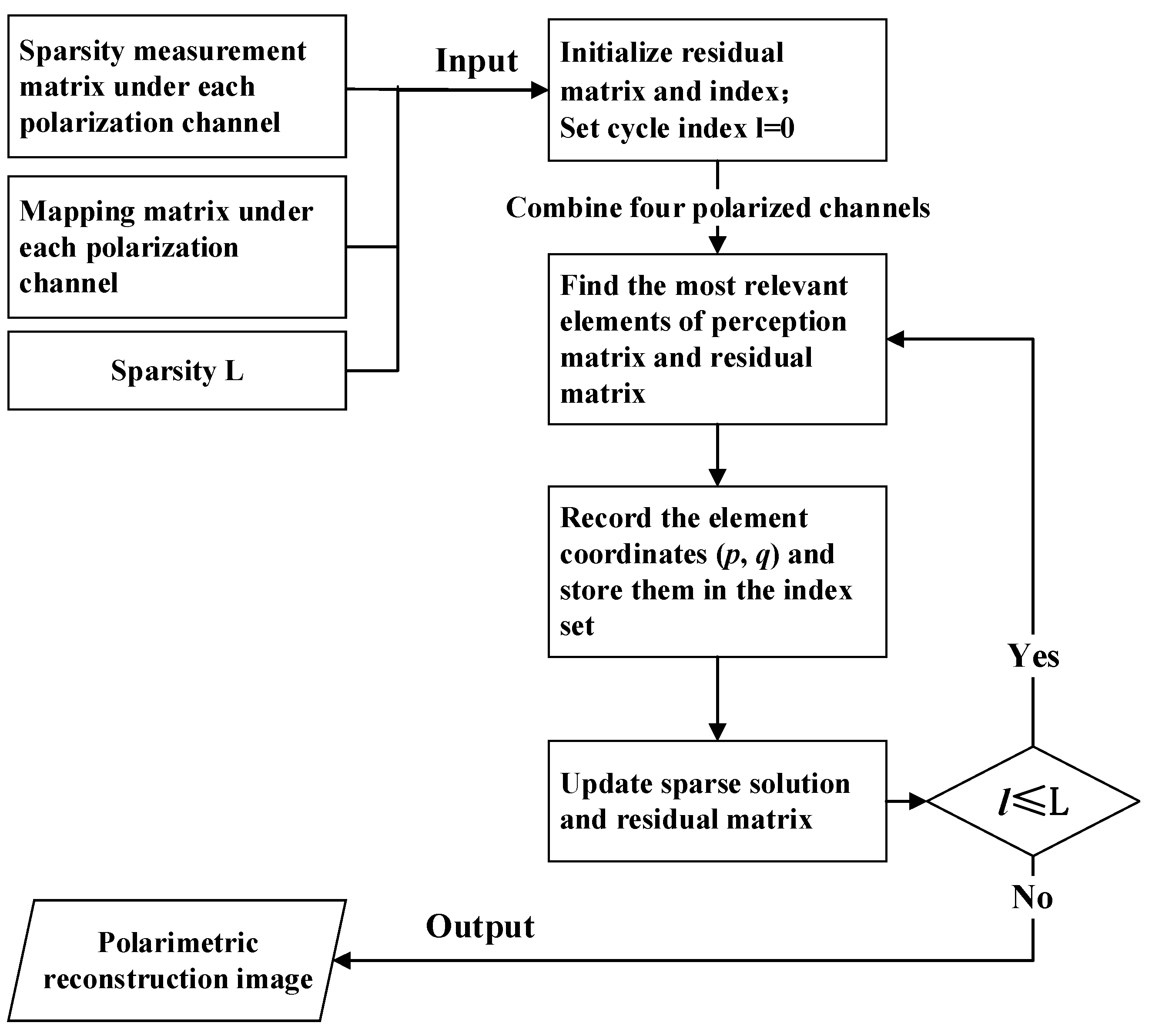
3.3. Procedure of the Proposed Reconstruction Algorithm

Similar to (5), each row of the sparse measured matrix ${\mathit{S}}_{f,k}$ is one measurement of the target; thus it is a multiple measurement vector (MMV) recovery problem [28,29]. In Section 3.1, we have already achieved an orthogonal coding aperture model. It is obvious that ${\mathit{S}}_{2D,k}$ satisfies row sparsity, which means its column vectors have non-zero elements at the same locations [30]. Taking advantage of the row sparsity property, many scholars have improved upon the OMP algorithm. The row-sparse mode is the simplest setting in MMVs. It can be solved by various approaches, such as simultaneous orthogonal matching pursuit (S-OMP) [30], an empirical Bayesian strategy [31] and simultaneous sparse Bayesian learning (SBL) [32], etc.

The S-OMP algorithm has the advantage of being computationally efficient, which facilitates the implementation of real-time image reconstruction. In contrast to the classical OMP algorithm, the S-OMP algorithm computes the sum of all basis vectors when finding the maximum relevant element. The intuition behind maximizing the sum of absolute correlations is to find an atom that can contribute a lot of energy to every column of the signal matrix. Inspired by the S-OMP algorithm, we propose a coded aperture simultaneous OMP (CAS-OMP) algorithm to solve the problem of orthogonal coded aperture reconstruction described above.

The algorithm flow chart is shown in Figure 6, and the specific algorithm steps are as follows.

Input: Slow-time range profile matrix ${\mathit{S}}_{f,k}$, sparse measurement matrix ${\mathit{\Phi }}_k$ and ISAR image sparsity L;

Output: ISAR images ${\mathit{S}}_{2D,k}$ to be reconstructed;

Step1: Initialize residual matrix ${\mathit{R}}_{0,k}={\mathit{S}}_{f,k}$, index set ${\mathit{\Lambda }}_0=$ Ø, and set cycle index $l=0$.

Step2: Calculate ${\displaystyle \sum _{k=1}^4\mathrm{abs}({{\mathit{\Phi }}_k}^H{\mathit{R}}_{l,k})}$. Find the coordinates $(p,q)$ of the largest element in ${\displaystyle \sum _{k=1}^4\mathrm{abs}({{\mathit{\Phi }}_k}^H{\mathit{R}}_{l,k})}$. Then update the index set ${\mathit{\Lambda }}_l={\mathit{\Lambda }}_{l-1}{{\displaystyle \cup }}^{ }\left\{\left(p,q\right)\right\}$.

Step3: Update the ISAR image ${\widehat{\mathit{S}}}_{2D,k}$, where the position of non-zero elements is determined by index set, and the scattering coefficient ${\mathit{\Gamma }}_k$ is calculated by the following method:Ŝ

Let ${\mathit{\Lambda }}_{l{q}_m}$ be the sequential subset of all the elements of index set ${\mathit{\Lambda }}_l$, whose column ordinal satisfies $q=q_m$. Where $q_m$ represents all the distinct column elements in ${\mathit{\Lambda }}_l$. The scattering coefficient ${\mathit{\Gamma }}_{k,q_m}$ was calculated by the least square method as follows:

$${\mathit{\Gamma }}_{k,q_m}={[{({\mathit{\Phi }}_{k,{\mathit{\Lambda }}_{l{q}_m}})}^H{\mathit{\Phi }}_{k,{\mathit{\Lambda }}_{l{q}_m}}]}^{-1}{{\mathit{\Phi }}_{k,{\mathit{\Lambda }}_{l{q}_m}}}^H{\mathit{S}}_{f,k{q}_m}$$

(15)

where ${\mathit{\Phi }}_{k,{\mathit{\Lambda }}_{l{q}_m}}$ is the column matrix in ${\mathit{\Lambda }}_{l{q}_m}$ obtained by indexing the row elements of ${\mathit{\Phi }}_k$, and ${\mathit{S}}_{f,k{q}_m}$ is the column vector indexed by $q_m$ in ${\mathit{S}}_{f,k}$.

Step4: Update residual matrix ${\mathit{R}}_{l,k}={\mathit{S}}_{f,k}-{\mathit{\Phi }}_k{\widehat{\mathit{S}}}_{2D,k}$. If $l\le L$,then back to Step2; Otherwise, stop the iteration, and output the ISAR image ${\mathit{S}}_{2D,k}$.

Where ${(\mathbf{·})}^H$ represents the transpose conjugate of the matrix.

The core of the CAS-OMP algorithm proposed is to calculate the sum of the absolute values of ${\mathit{\Phi }}_k^H{\mathit{R}}_{l,k}$ in the four channels in step 2. Since the scattering points of the reconstructed images in different polarization channels are consistent, we considered summing up the relevant results of the measurement matrix and residual matrix in the four polarization channels to obtain their common maximum element and obtain their index coordinates. Distinguishing from the S-OMP algorithm in which all sparse measurement matrices are kept consistent, the measurement matrices in this algorithm are two by two identical. That is, ${\mathit{\Phi }}_1={\mathit{\Phi }}_2$ and ${\mathit{\Phi }}_3={\mathit{\Phi }}_4$, as mentioned above. The proposed method can ensure the consistency of the scattering points in all polarization channels. It is beneficial to the subsequent polarization feature extraction and target recognition. In addition, for the weak scattering points in cross-polarized channel, the joint processing can make full use of the scattering information in the co-polarized channel. This ensures the successful reconstruction of the scattering points in the cross-polarized channel.

4. Simulation and Analysis

4.1. Numerical Simulation

In this section, an experiment based on simulation data is conducted to verify the effectiveness of the proposed method. The experiments were carried out in MATLAB R2020b on a computer equipped with an AMD Ryzen 7 5800H CPU and 12 GB of RAM. The echo data was generated by MATLAB, using the 80-point ideal scattering model of a satellite, with a wingspan of 20 m and a height of 15 m. The scattering point model is shown in Figure 7.

4.1.1. Parameter Setting and Reconstruction Images

The X-band full-polarization imaging radar with a carrier frequency of 10 GHz was set in the simulation, and the specific signal parameter setting is shown in

Table 1. Radar parameter setting.

Parameter Setting	Value
carrier frequency f0	10 GHz
pulse width Tp	100 $\mathsf{\mu }\mathrm{s}$
bandwidth B	500 MHz
azimuth pulse number	256
distance sampling number	1024
pulse repetition interval	1 ms
polarization mode	HH\HV\VH\VV

.

$100 \mathsf{\mu }\mathrm{s}$ The signal-to-noise ratio (SNR) is set to −10 dB and the sparsity L = 200. The ISAR images obtained according to the traditional range-Doppler algorithm (RD algorithm) are shown in Figure 8a–d. In addition, the ISAR images obtained by the multichannel joint reconstruction method are shown in Figure 8e–h. The different colors of scattering points in Figure 8 represent the difference in amplitude between them. Yellow represents a large amplitude, while blue represents a small amplitude. The scattering intensity of each scattering point set in this simulation can be seen intuitively in Figure 8a–d. It can be seen that the reconstructions of all channels are successful, although the intensity of scattering points in the cross-polarized channel is significantly weaker than that in the co-polarized channel. The relative intensity of scattered points after sparse reconstruction by the proposed method is consistent with the original simulation setting.

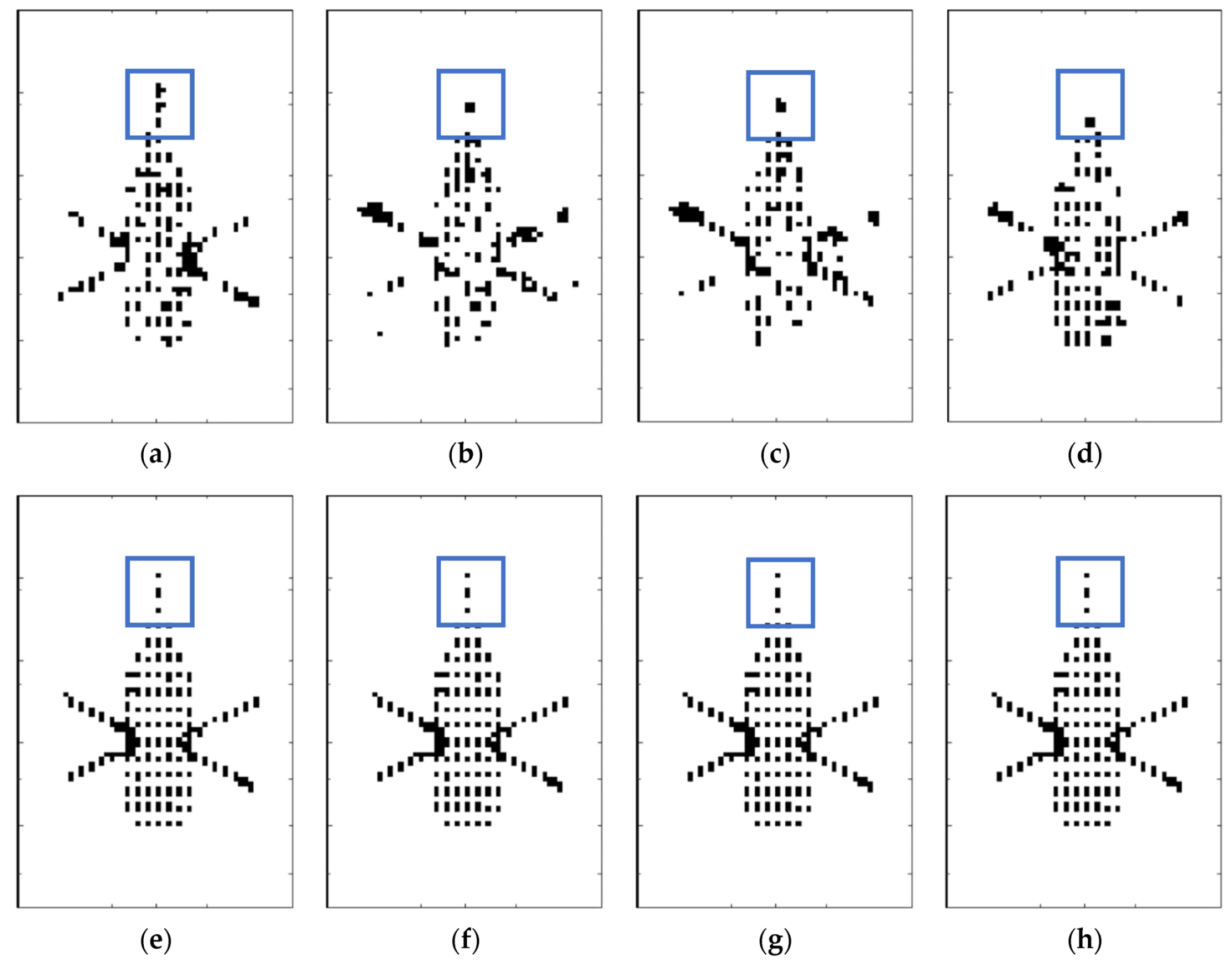
4.1.2. Consistency of Reconstruction Images

Multichannel joint reconstruction can make use of the correlation information of different polarization channels to ensure the consistency of the reconstructed scattering points of each polarization channel. Figure 9 compares the reconstruction results of four polarization channels in two different ways. All the parameters are set in the same way. Figure 9a–d show the images reconstructed independently by each polarization channel, while Figure 9e–h show the joint reconstruction images of four polarization channels. In order to enhance the display visibility, the reconstructed image matrixes were mapped to 0-1 matrixes. The elements of the matrix corresponding to the scattering points was set as 1, and the others were set as 0. The reconstruction results are displayed in grayscale. As shown in Figure 9, the positions of the scattering points in four polarization channels are different when each polarization channel is reconstructed separately. In comparison, the positions of the scattering points in the four channels remain the same when multichannel joint reconstruction is conducted. It can be seen clearly from Figure 9a–d that there exist some scattering points that have not been reconstructed in the image of each polarization channel, while some nonexistent scattering points have been incorrectly reconstructed. It has been proven that the proposed algorithm is effective in guaranteeing the consistency of scattering points in different polarization channels. Furthermore, it also improves the quality of reconstructed images.

4.1.3. Reconstructed Image Quality

In order to evaluate the quality of image reconstruction, image entropy and image contrast are used for quantitative evaluation [33].

Image Entropy

Image entropy is defined as follows:

$$S=\stackrel{\underset{N}{n=1}}{{{\displaystyle \sum }}^{ }}\stackrel{\underset{M}{m=1}}{{{\displaystyle \sum }}^{ }}D\left(n,m\right)\ln D\left(n,m\right)$$

(16)

where D (n, m) represents the normalized image, which is given by:

$$D\left(n,m\right)=\frac{I{(n,m)}^2}{\stackrel{\underset{N}{n=1}}{{{\displaystyle \sum }}^{ }}\stackrel{\underset{M}{m=1}}{{{\displaystyle \sum }}^{ }}I{(n,m)}^2}$$

(17)

where I (n, m) represent the intensity of pixels in an image.

The H-polarization and V-polarization channel sequences of orthogonal coding aperture were generated according to the modulation parameters randomly. When calculating the ISAR image entropy, five experiments with different pseudo-random coding sequences were conducted. The ISAR image entropy obtained is shown in

Table 2. ISAR reconstructed image entropy.

Reconstruction Algorithm	Polarization Channel	Experiment Serial Number					Average Image Entropy
		1	2	3	4	5
RD algorithm	HH channel	5.955	5.785	5.710	5.809	5.803	5.813
	HV channel	4.498	4.782	4.565	4.471	3.982	4.460
	VH channel	4.518	4.739	4.636	4.476	4.024	4.479
	VV channel	5.850	5.983	5.876	5.866	5.758	5.867
Full-polarization joint reconstruction algorithm	HH channel	0.706	0.696	0.707	0.700	0.701	0.702
	HV channel	0.663	0.683	0.670	0.660	0.644	0.664
	VH channel	0.674	0.673	0.674	0.657	0.639	0.663
	VV channel	0.696	0.697	0.704	0.704	0.705	0.701

. SNR is set to −10 dB, and sparsity L = 200.

It is known that an image with better focusing performance corresponds to a lower image entropy [34]. As shown in Table 2, the radar images reconstructed jointly have smaller image entropy compared to the image obtained using the traditional RD algorithm. Combining with Figure 8, it is obvious that the reconstruction results using the RD algorithm contain a lot of noise under the condition of −10 dB SNR. In comparison, the images obtained using the multichannel joint reconstruction method only have strong scattered points. By comparing the average image entropy of the images obtained by these two algorithms, the difference between the co-polarization channel and the cross-polarization channel is smaller when applying the joint reconstruction method. This proves that the correlation information between multiple channels is used in the reconstruction, resulting in better image quality in the cross-polarization channel.

Image Contrast

The gray gradient level of an image can be quantitatively characterized by calculating the image contrast. The definition of contrast is as follows:

$$C=\underset{\delta }{{{\displaystyle \sum }}^{ }}\delta {(i,j)}^2{P}_{\delta }\left(i,j\right)$$

(18)

where $\delta (i,j)=|i-j|$ represents the gray difference between adjacent pixels, and $P_{\delta }(i,j)$ represents the probability of pixel distribution. In this paper, the adjacent pixels were taken eight adjacent pixels around the current pixel. The SNR is set to −10 dB, and the sparsity L = 200.

The greater the image contrast, the better observability can be obtained. As shown in

Table 3. ISAR-reconstructed image contrast.

Reconstruction Algorithm	Polarization Channel	Experiment Serial Number					Average Image Contrast
		1	2	3	4	5
RD algorithm	HH channel	347.839	307.060	273.733	295.230	303.917	305.556
	HV channel	153.530	168.654	164.888	151.233	136.719	155.005
	VH channel	156.150	166.363	163.592	149.898	136.994	154.600
	VV channel	301.904	335.617	304.306	312.230	287.988	308.409
Full-polarization joint reconstruction algorithm	HH channel	499.981	435.572	411.414	444.382	423.317	442.933
	HV channel	188.784	201.384	180.080	162.159	148.806	176.242
	VH channel	190.817	196.223	181.416	166.137	146.995	176.317
	VV channel	452.815	510.040	510.289	467.005	493.793	486.788

, the image contrast obtained by the multichannel joint reconstruction algorithm is improved compared with the traditional method, especially in the co-polarization channel. This indicates that the proposed algorithm can obtain better radar image than the RD imaging algorithm.

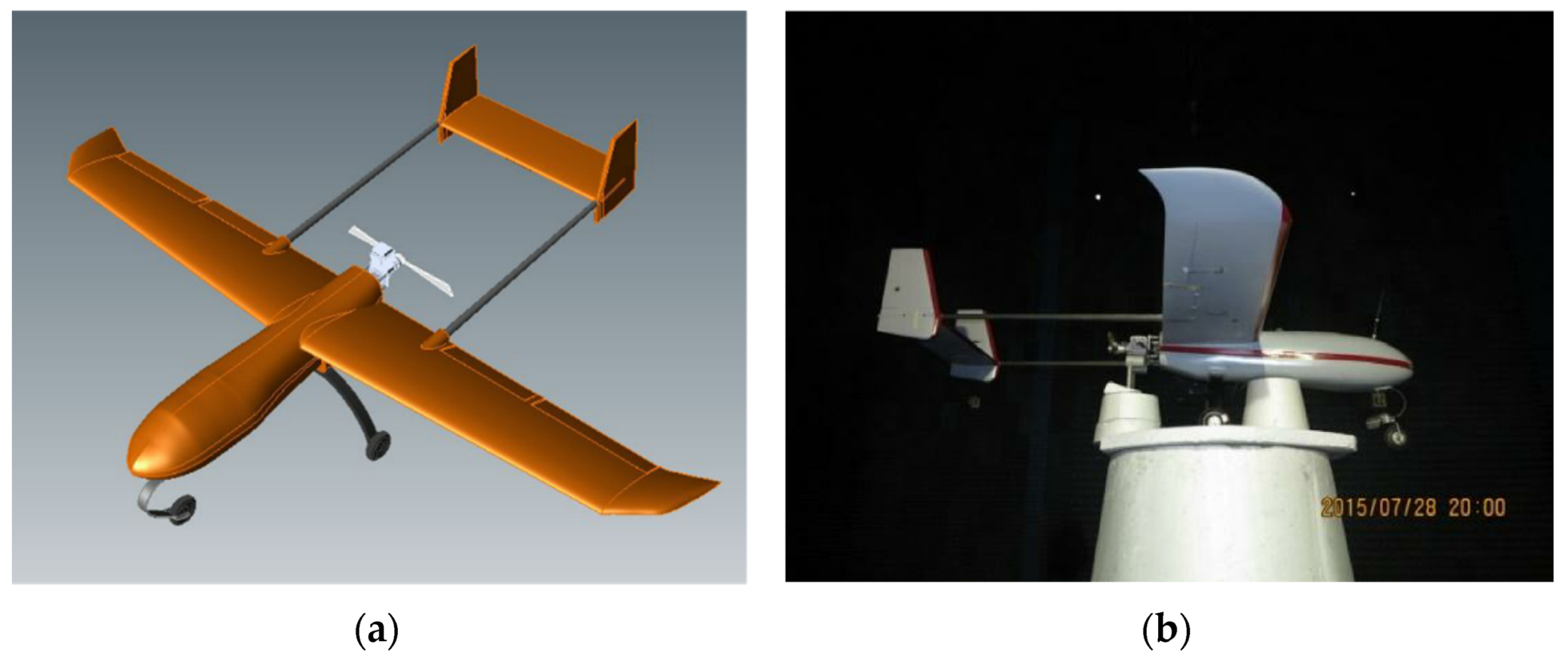
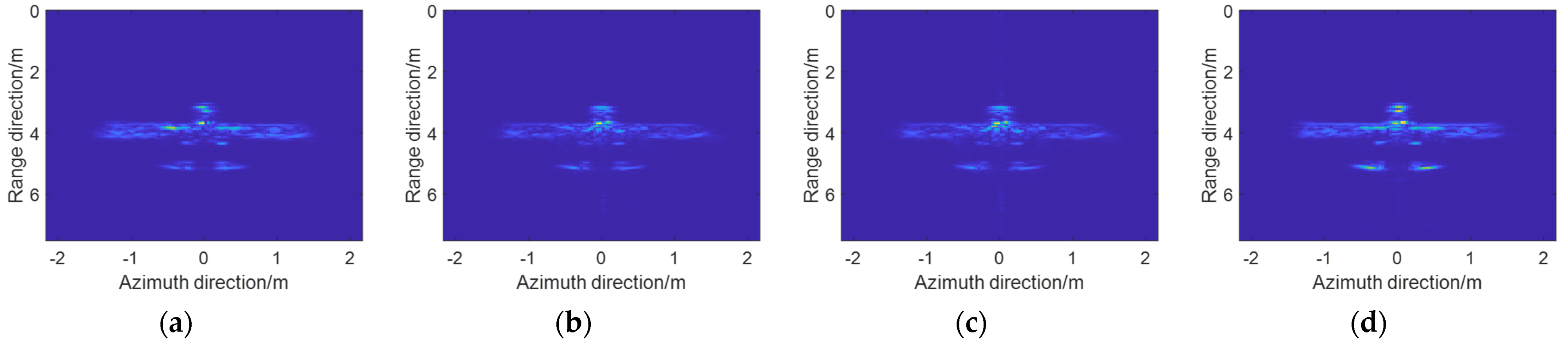
4.2. Measured Data Simulation

On the basis of numerical simulation, the effectiveness of the proposed CAS-OMP algorithm is further verified by the measured unmanned aerial vehicle (UAV) data in a microwave anechoic chamber.

The ‘pioneer’ UAV model used here is shown in Figure 10a, and the measured scene setting of UAV in microwave anechoic chamber is shown in Figure 10b. The UAV has a length of 2.3 m, a wingspan of 2.9 m and a height of 0.66 m. The nose direction is placed along the X-axis, defined as 0° in the azimuth direction.

The full-polarization data of the UAV was obtained by static measurement of complete sweep signal. The parameters of sweep signal are shown in the table below. As shown in

Table 4. Parameters of sweep signal.

Parameter Setting	Value
initial frequency	8 GHz
terminal frequency	12 GHz
bandwidth B	4 GHz
frequency interval	20 MHz
number of sub pulses	200
pitch angle	0°
azimuth angle	−180°~180°
azimuth interval	0.2°

, the complete sweep signal consists of 200 sub pulses with a frequency range from 8 GHz to 12 GHz and bandwidth of 4 GHz.

The UAV imaging results in all polarization channels using the RD algorithm are shown in Figure 11. The nose, wings and landing gear of the UAV can be distinguished from Figure 11. All the measured data of the UAV are taken as a complete data set. On this basis, we extract the coded aperture of the UAV echo data in azimuth upward with 50% sparsity, so as to simulate the echo received by alternately transmitting H and V polarization signals according to the coding sequence.

After extracting the coded aperture from the complete echo data, we obtained the sparse aperture echo data of UAV in four polarization channels. Then we used the RD algorithm and CAS-OMP algorithm proposed in this paper for imaging, and the sparsity L was set to 750. The imaging results are shown in Figure 12.

As shown in Figure 12a–d, when the conventional RD algorithm is applied, the images have a serious defocus, especially the part of the wing with a long extension in the azimuth, which affects the measurement accuracy of the imaging results. However, it can be seen from Figure 12e–h that the UAV image was reconstructed successfully using CAS-OMP algorithm, and it is obviously better than that using the RD algorithm. The imaging results using CAS-OMP algorithm are basically similar to imaging results using RD algorithm with a complete data set. Hence, this proves the effectiveness of proposed reconstruction algorithm.

5. Conclusions

In this paper, an orthogonal coding aperture model is proposed for full-polarization radar imaging. Accordingly, a joint image reconstruction algorithm called the CAS-OMP algorithm is proposed. The numerical simulations and the imaging results of measured UAV data show that the correlation information between different polarization channels is utilized by the proposed method. The image in the cross-polarized channel can be obtained with better reconstruction quality, which proves the effectiveness of the proposed method.

Future work will focus on the following three aspects. Firstly, studies on the code sequence design and optimization will be conducted to obtain better reconstruction performance. Then the theoretical performance and applicable conditions of the proposed CAS-OMP algorithm will be further analyzed. Furthermore, experiments based on radar systems will be carried out to further verify the effectiveness of this algorithm in real scenarios.

References

1. Ender, J.; Amin, M.; Fornaro, G.; Rosen, P.A. Recent Advances in Radar Imaging [From the Guest Editors]. IEEE Signal Process. Mag. 2014, 31, 15–158. [Google Scholar] [CrossRef]
2. Kuenzer, C.; Bluemel, A.; Gebhardt, S.; Quoc, T.V.; Dech, S. Remote Sensing of Mangrove Ecosystems: A Review. Remote Sens. 2011, 3, 878–928. [Google Scholar] [CrossRef] [Green Version]
3. Radecki, K.; Samczynski, P.; Gromek, D. Fast Barycentric-Based Back Projection Algorithm for SAR Imaging. IEEE Sens. J. 2019, 19, 10635–10643. [Google Scholar] [CrossRef]
4. Ao, D.; Wang, R.; Hu, C.; Li, Y. A Sparse SAR Imaging Method Based on Multiple Measurement Vectors Model. Remote Sens. 2017, 9, 297. [Google Scholar] [CrossRef] [Green Version]
5. Xu, X.; Narayanan, R.M. Enhanced resolution in SAR/ISAR imaging using iterative sidelobe apodization. IEEE Trans. Image Process. 2005, 14, 537–547. [Google Scholar] [CrossRef]
6. Bai, X.R. Study on New Techniques for ISAR Imaging of Aerospace Targets. Ph.D. Dissertation, Xidian University, Xi’an, China, 2014. [Google Scholar]
7. Kang, M.-S.; Bae, J.-H.; Lee, S.-H.; Kim, K.-T. Efficient ISAR autofocus via minimization of Tsallis Entropy. IEEE Trans. Aerosp. Electron. Syst. 2017, 52, 2950–2960. [Google Scholar] [CrossRef]
8. Tian, B.; Liu, Y.; Hu, P.J. Review of high-resolution imaging techniques of wideband inverse synthetic aperture radar. J. Radars 2020, 9, 765–802. [Google Scholar] [CrossRef]
9. Wang, Y.; Liu, H.; Jiu, B. PolSAR Coherency Matrix Decomposition Based on Constrained Sparse Representation. IEEE Trans. Geosci. Remote Sens. 2014, 52, 5906–5922. [Google Scholar] [CrossRef]
10. Guo, H.D. Earth Observation Technology and Sustainable Development; Science Press: Beijing, China, 2001. [Google Scholar]
11. Jin, Y.Q.; Xu, F. Theory and Approach for Polarimetric Scattering and Information Retrieval of SAR Remote Sensing; Science Press: Beijing, China, 2008. [Google Scholar]
12. Chen, S.W.; Wang, X.S.; Xiao, S.P. Target Scattering Mechanism in Polarimetric Synthetic Aperture Radar: Interpretation and Application; Springer: Singapore, 2018. [Google Scholar]
13. Migliaccio, M.; Gambardella, A.; Tranfaglia, M. SAR Polarimetry to Observe Oil Spills. IEEE Trans. Geosci. Remote Sens. 2007, 45, 506–511. [Google Scholar] [CrossRef]
14. De Maio, A.; Orlando, D.; Pallotta, L.; Clemente, C. A Multifamily GLRT for Oil Spill Detection. IEEE Trans. Geosci. Remote Sens. 2016, 55, 63–79. [Google Scholar] [CrossRef]
15. Dai, H.; Wang, X.; Li, Y.; Liu, Y.; Xiao, S. Main-Lobe Jamming Suppression Method of using Spatial Polarization Characteristics of Antennas. IEEE Trans. Aerosp. Electron. Syst. 2012, 48, 2167–2179. [Google Scholar] [CrossRef]
16. Dai, H.; Chang, Y.; Dai, D.; Li, Y.; Wang, X. Calibration method of phase distortions for cross polarization channel of instantaneous polarization radar system. J. Syst. Eng. Electron. 2010, 21, 211–218. [Google Scholar] [CrossRef]
17. Giuli, D.; Facheris, L.; Fossi, M.; Rossettini, A. Simultaneous scattering matrix measurement through signal coding. In Proceedings of the IEEE International Conference on Radar, Arlington, VA, USA, 7–10 May 1990. [Google Scholar] [CrossRef]
18. Zhang, Y.J.; Li, C.P. Analysis of synthetic aperture radar ambiguities. J. Electro. Inf. Technol. 2004, 26, 1455–1460. [Google Scholar]
19. Donoho, D.L. Compressed sensing. IEEE Trans. Inf. Theory 2006, 52, 1289–1306. [Google Scholar] [CrossRef]
20. Candes, E.; Romberg, J.; Tao, T. Robust uncertainty principles: Exact signal reconstruction from highly incomplete frequency information. IEEE Trans. Inf. Theory 2006, 52, 489–509. [Google Scholar] [CrossRef] [Green Version]
21. Candes, E.J.; Wakin, M. An Introduction to Compressive Sampling. IEEE Signal Process. Mag. 2008, 25, 21–30. [Google Scholar] [CrossRef]
22. Hu, C.; Wang, L.; Zhu, D.; Loffeld, O. Inverse Synthetic Aperture Radar Sparse Imaging Exploiting the Group Dictionary Learning. Remote Sens. 2021, 13, 2812. [Google Scholar] [CrossRef]
23. Liu, H.C. Study on New Method of High Resolution ISAR Imaging. Ph.D. Dissertation, Xidian University, Xi’an, China, 2014. [Google Scholar]
24. Zhang, L.; Wu, S.; Duan, J. Sparse-aperture ISAR imaging of maneuvering targets with sparse representation. In Proceedings of the 2015 IEEE Radar Conference (RadarCon), Arlington, VA, USA, 10–15 May 2015; pp. 1623–1626. [Google Scholar] [CrossRef]
25. Bi, H.; Zhu, D.; Bi, G.; Zhang, B.; Hong, W.; Wu, Y.-R. FMCW SAR Sparse Imaging Based on Approximated Observation: An Overview on Current Technologies. IEEE J. Sel. Top. Appl. Earth Obs. Remote Sens. 2020, 13, 4825–4835. [Google Scholar] [CrossRef]
26. Wu, Q.; Liu, X.; Liu, J.; Zhao, F.; Xiao, S. A Radar Imaging Method Using Nonperiodic Interrupted Sampling Linear Frequency Modulation Signal. IEEE Sensors J. 2018, 18, 1. [Google Scholar] [CrossRef]
27. Zhuang, Z.W.; Xiao, S.P.; Wang, X.S. Radar Polarization Information Processing and Application; National Defense Industry Press: Beijing, China, 1999. [Google Scholar]
28. Chen, J.; Huo, X. Sparse Representations for Multiple Measurement Vectors (MMV) in an Over-Complete Dictionary. In Proceedings of the IEEE International Conference on Acoustics, Speech, and Signal Processing, Philadelphia, PA, USA, 23 March 2005. [Google Scholar]
29. Chen, J.; Huo, X. Theoretical Results on Sparse Representations of Multiple-Measurement Vectors. IEEE Trans. Signal Process. 2006, 54, 4634–4643. [Google Scholar] [CrossRef] [Green Version]
30. Tropp, J.; Gilbert, A.C.; Strauss, M.J. Algorithms for simultaneous sparse approximation. Part I: Greedy pursuit. Signal Process. 2006, 86, 572–588. [Google Scholar] [CrossRef]
31. Wipf, D.P.; Rao, B.D. An Empirical Bayesian Strategy for Solving the Simultaneous Sparse Approximation Problem. IEEE Trans. Signal Process. 2007, 55, 3704–3716. [Google Scholar] [CrossRef]
32. Chen, W.; Wipf, D.; Wang, Y.; Liu, Y.; Wassell, I.J. Simultaneous Bayesian Sparse Approximation with Structured Sparse Models. IEEE Trans. Signal Process. 2016, 64, 6145–6159. [Google Scholar] [CrossRef] [Green Version]
33. Wang, Z.; Bovik, A.C.; Sheikh, H.R.; Simoncelli, E.P. Image Quality Assessment: From Error Visibility to Structural Similarity. IEEE Trans. Image Process. 2004, 13, 600–612. [Google Scholar] [CrossRef] [PubMed] [Green Version]
34. Cao, P.; Xing, M.; Sun, G.; Li, Y.; Bao, Z. Minimum Entropy via Subspace for ISAR Autofocus. IEEE Geosci. Remote Sens. Lett. 2009, 7, 205–209. [Google Scholar] [CrossRef]
Figure 1. ISAR imaging geometry.
Remotesensing 13 04626 g001
Figure 2. Two different aperture arrangements: (a) uniform alternating aperture; (b) orthogonal coding apertures.
Remotesensing 13 04626 g002
Figure 3. Imaging results of Yake-42 simulation model under different aperture extraction ratio: (a) Yake-42 simulation model; (b) Aperture extraction ratio 100%; (c) Aperture extraction ratio 75%; (d) Aperture extraction ratio 50%.
Remotesensing 13 04626 g003
Figure 4. Orthogonal coding aperture model.
Remotesensing 13 04626 g004
Figure 5. Distribution of scattered points in each channel.
Remotesensing 13 04626 g005
Figure 6. Flow chart of reconstruction algorithm.
Remotesensing 13 04626 g006
Figure 7. Satellite scattering point simulation model.
Remotesensing 13 04626 g007
Figure 8. Comparison of reconstructed image between RD algorithm and CS algorithm: (ad) represent the images obtained by RD algorithm in HH, HV, VH and VV polarization channels, respectively; (eh) represent the images obtained by CS algorithm in HH, HV, VH and VV polarization channels, respectively.
Remotesensing 13 04626 g008
Figure 9. Mapping images of single-channel reconstruction and multichannel joint reconstruction: (ad) represent the single-channel reconstruction images in HH, HV, VH and VV polarization channels, respectively; (eh) represent the multichannel joint reconstruction images in HH, HV, VH and VV polarization channels, respectively. Notice that the blue boxes mark the scattering points at the same location in the different images. It is clear that the positions of the scattering points differ from each other when each polarization channel is reconstructed separately. In contrast, the positions of the scattering points from the joint reconstruction results remain consistent within each channel.
Remotesensing 13 04626 g009
Figure 10. (a) ‘Pioneer’ UAV model; (b) Measurement scene in the microwave anechoic chamber.
Remotesensing 13 04626 g010
Figure 11. UAV imaging results using RD algorithm: (a) HH polarization channel; (b) HV polarization channel; (c) VH polarization channel; (d) VV polarization channel.
Remotesensing 13 04626 g011
Figure 12. Imaging results of UAV with sparse aperture extraction: (ad) represent the imaging results using RD algorithm in HH, HV, VH and VV polarization channels, respectively; (eh) represent the imaging results using CAS-OMP algorithm in HH, HV, VH and VV polarization channels, respectively.
Remotesensing 13 04626 g012