Abstract
Object localization is an important application of remote sensing images and the basis of information extraction. The acquired accuracy is the key factor to improve the accuracy of object structure information inversion. The floating roof oil tank is a typical cylindrical artificial object, and its top cover fluctuates up and down with the change in oil storage. Taking the oil tank as an example, this study explores the localization by combining the traditional feature parameter method and convolutional neural networks (CNNs). In this study, an improved fast radial symmetry transform (FRST) algorithm called fast gradient modulus radial symmetry transform (FGMRST) is proposed and an approach based on FGMRST combined with CNN is proposed. It effectively adds the priori of circle features to the calculation process. Compared with only using CNN, it achieves higher precision localization with fewer network layers. The experimental results based on SkySat data show that the method can effectively improve the calculation accuracy and efficiency of the same order of magnitude network, and by increasing the network depth, the accuracy still has a significant improvement.
1. Introduction
In computer vision, object localization is to determine the position of the object in a single object image, and object detection is to identify all the objects and determine their positions in an image in which the type and number of objects are not fixed. In recent years, object localization in remote sensing images has been widely used in the investigation of agriculture and forestry, urban surveying, marine monitoring, and military reconnaissance [1,2]. The circle is a basic shape of objects in 2D images. Its localization technology is an important task in computer vision and pattern recognition, and it is also a hot research topic at home and abroad. The floating roof oil tank in remote a sensing image, as a representative of a man-fabricated object with the circular feature, plays an important role in both military and civil fields [3].
The position of the top cover of the floating roof oil tank fluctuates up and down with the change in oil storage, so the remote sensing image of the oil tank has different circular shadows and multiple circular areas. The localization of the oil tank in this study refers to the determination of the center position of the tank roof, the center position of the circular-arc-shaped shadow cast by the sun on the floating roof, and the radius of the oil tank in the image, which is of great significance for the inversion of the oil tank structure [4] and the oil storage information [5].
There are two kinds of methods for localizing the circle center. One is the traditional parameterized feature extraction method, including the method based on Hough transform [6] and the method based on template matching [7,8]. Han et al. [9] improved Hough transform by using the gradient direction information and reducing the dimension of parameter space, and then combined the graph search strategy to act on an oil tank [10]. Zhang et al. [11] used the improved random Hough transform (RHT), improved Canny algorithm, and template matching algorithm to deal with an oil tank. The other is the emerging deep learning [12] method. It transforms the raw data into abstract high-level representation through a nonlinear model to discover the distributed feature representation of the data [13,14]. In 1989, LeCun et al. [15] proposed convolutional neural networks (CNNs). In 2012, the deep CNN model built by Hinton et al. achieved state-of-the-art results in the ImageNet competition [16], which attracted extensive attention from industry and academia. In 2015, ResNet proposed by He et al. [17] won three championships of image detection, image classification, and image localization in the ImageNet Large Scale Visual Recognition Challenge (ILSVRC) competition, which exceeded the accuracy of human recognition for the first time [18].
In response to the problem of localization of the oil tank in remote sensing images, the two methods mentioned above have their own advantages and disadvantages. The traditional parameterized feature extraction method makes effective use of the circumference feature, but it is not learnable, and the applicability of parameters is poor. It needs to rely on experience or priori knowledge to continuously adjust parameters manually, and the degree of automation is low. The method based on deep learning is an end-to-end method. However, in the face of an object with a circular structure such as an oil tank, it is unable to fully explore the unique patterns of data and requires a large receptive field. Therefore, it needs to increase the receptive field by cascading multiple networks, which leads to a great increase in its parameters and computation. Based on this, this study aims to make effective use of the priori features while adding the learning features of the existing data to reduce the amount of calculation and improve accuracy and efficiency. We propose a new method combining the above two methods.
This study discusses the coverage of the receptive field of the CNN method and proposes the fast gradient modulus radial symmetry transform (FGMRST) based on the characteristics of the oil tank image and the fast radial symmetry transform (FRST) [19]. We use FGMRST to realize the spatial region aggregation of circular features and construct a method combining FGMRST and CNN. This method can efficiently aggregate spatial features and improve the accuracy and efficiency of the network. We carried out verification experiments based on the data of the SkySat satellite [20]. The results show that, compared with ordinary CNN, the method can effectively improve the accuracy of the localization of the oil tank, and has good stability.
2. Methods
2.1. CNN-Based Localization Method of the Oil Tank
As a kind of supervised deep feedforward neural networks with convolution, CNN has been widely concerned and applied because of its excellent performance in the field of computer vision, and is one of the representative algorithms of deep learning. The main idea of the CNN-based localization method of oil tank is: using CNN to train the five parameters of the remote sensing image, which are the X and Y coordinates of the center of the tank roof, the X and Y coordinates of the center of the circular-arc-shaped shadow cast by the sun on the floating roof and the radius of the oil tank, and obtain their predictive values through regression. In the face of the localization of the oil tank, CNN can predict the radius and obtain an accurate location of the circle center. However, its disadvantages are obvious:
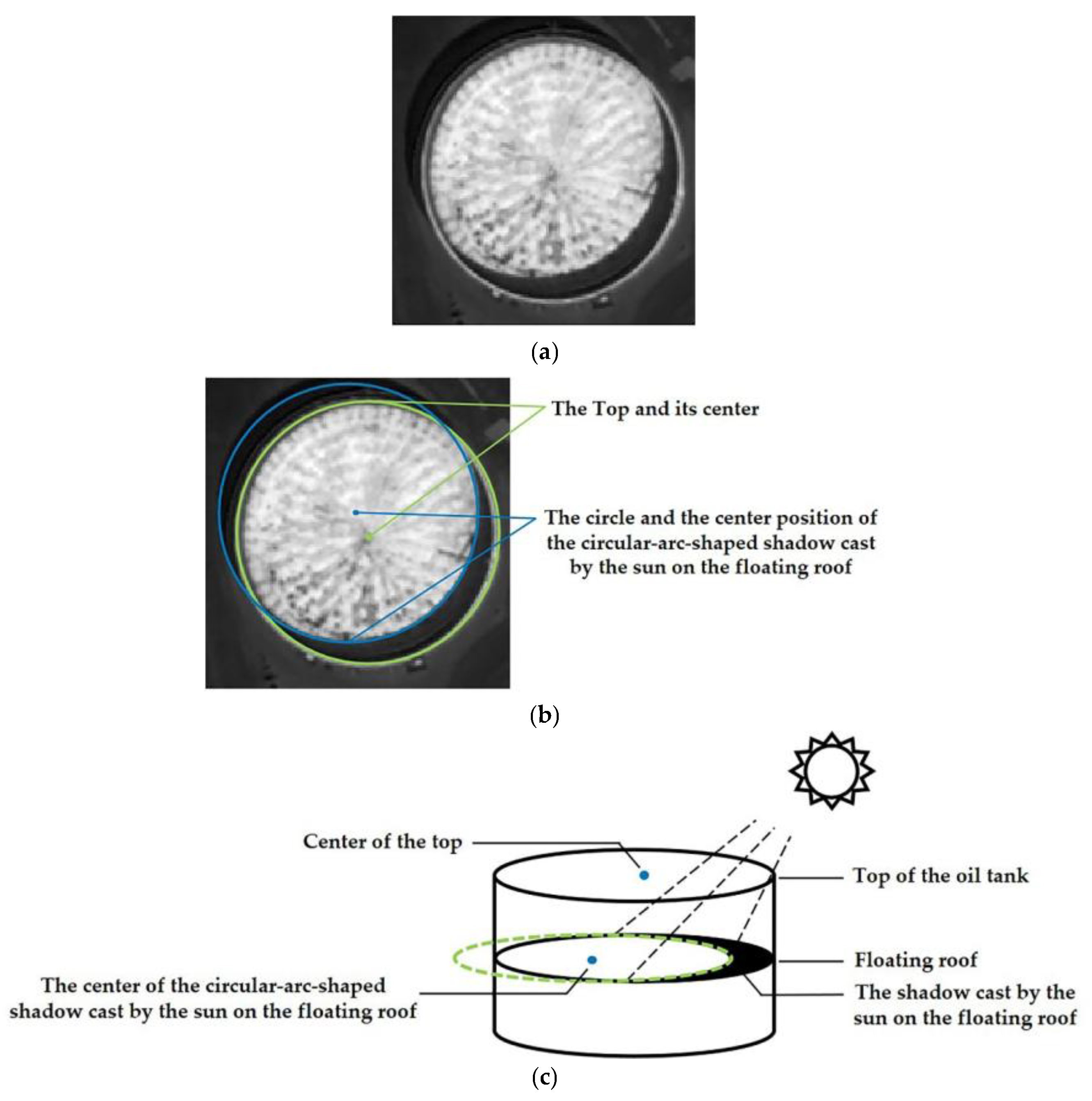
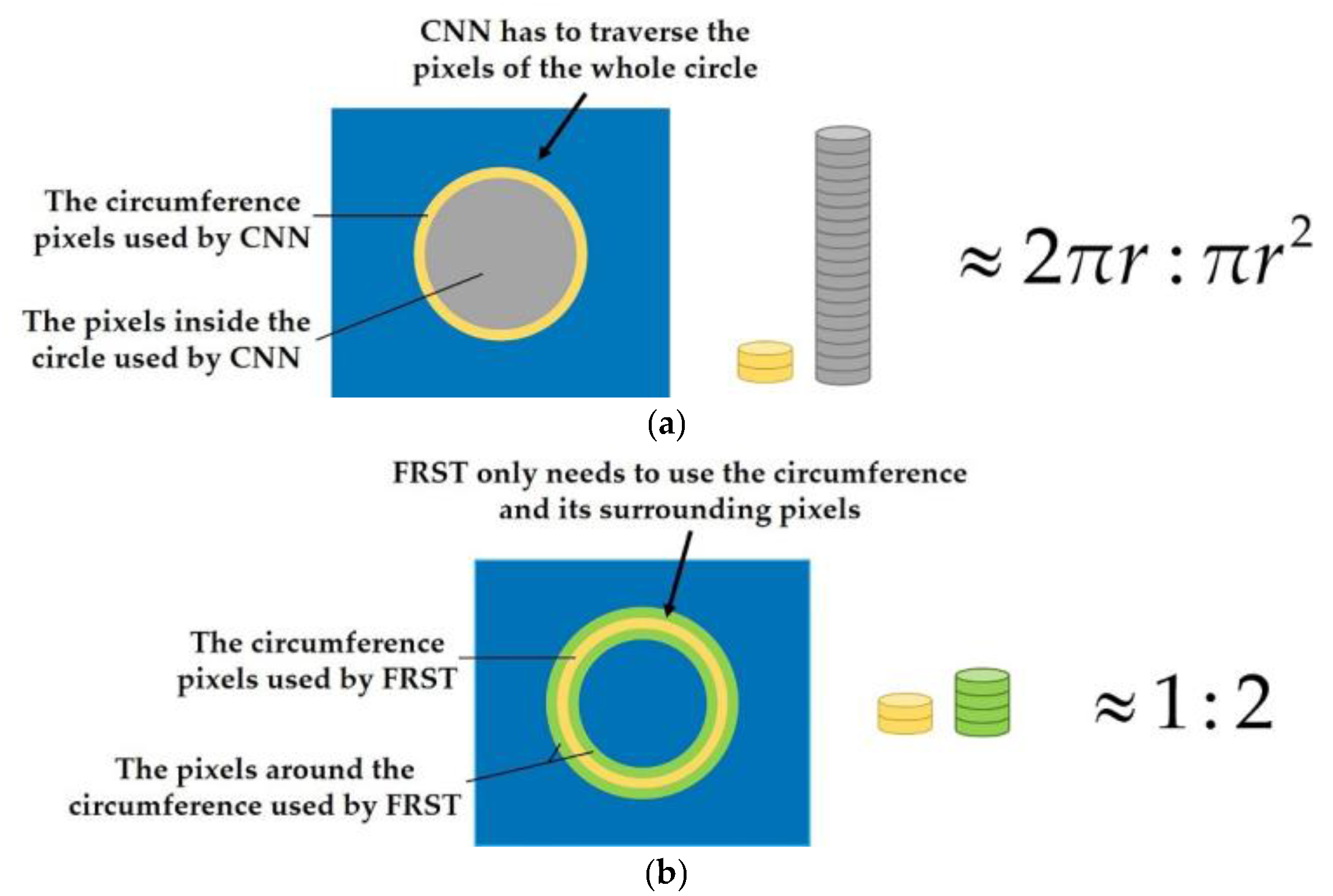
- The main feature of an object with a circular structure such as the oil tank is on the circumference, but not in the circle (as shown in Figure 1). However, at present, the neural networks need to traverse all the pixels (as shown in Figure 2a), which leads to a large increase in unnecessary computation and a low processing efficiency.
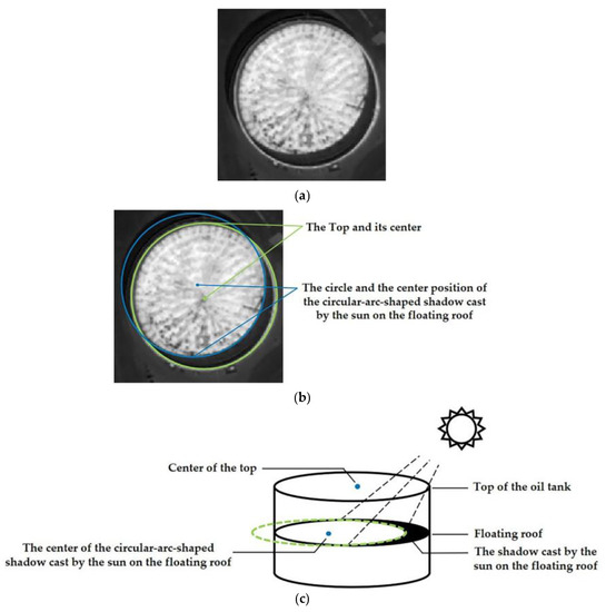 Figure 1. Structural diagram of floating roof oil tank. (a) Original image; (b) top of oil tank and circle of circular arc on the floating roof; (c) three-dimensional structure of floating roof oil tank.
 Figure 2. Comparison of the number of pixels traversed by CNN and FRST to process circular objects. (a) Comparison of the number of pixels traversed by CNN in processing circular objects; (b) comparison of the number of pixels traversed by FRST in processing circular objects
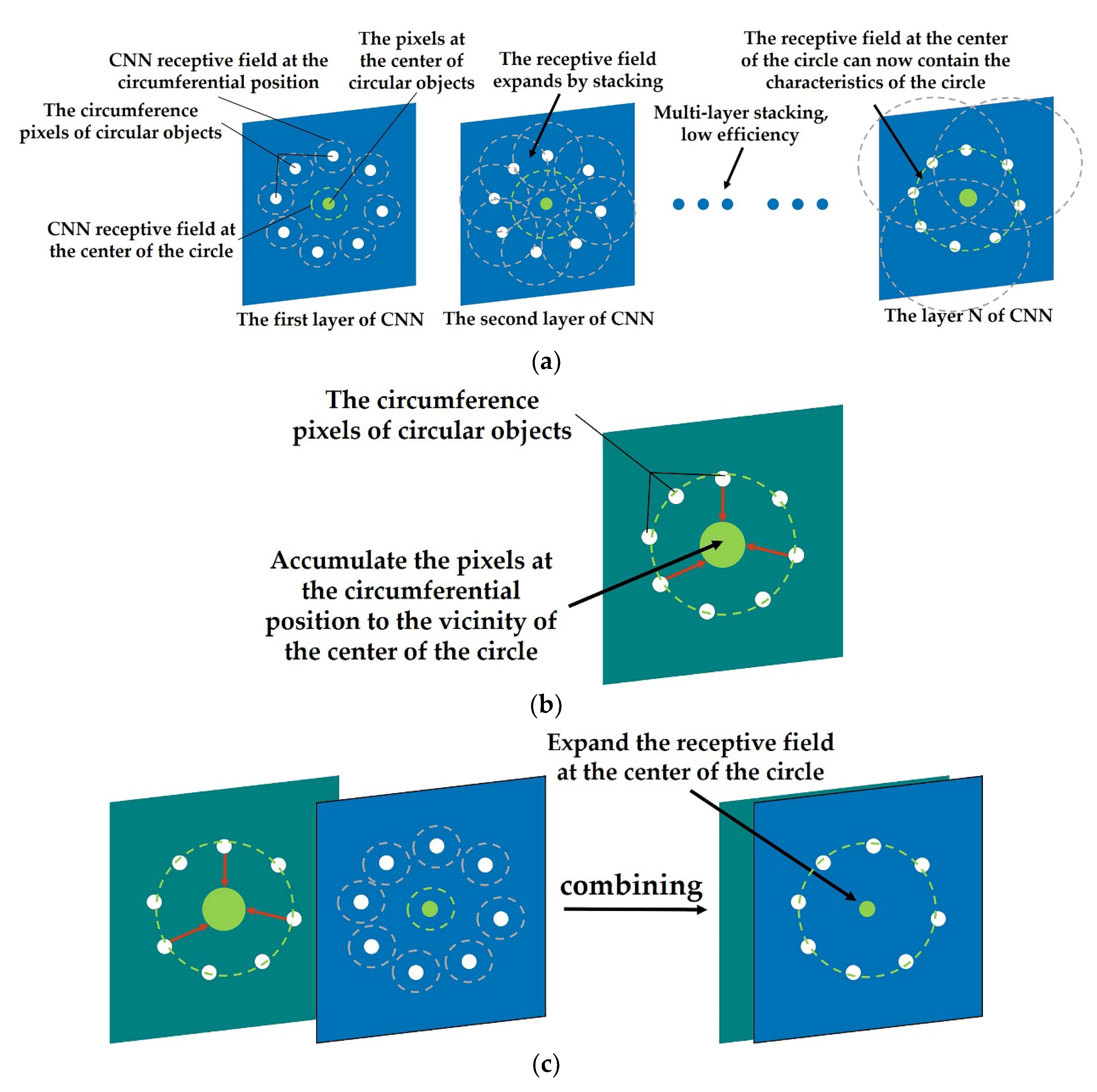
 - Due to the limitation of the receptive field, CNN gradually increases the receptive field and aggregates the spatial features by cascading networks (as shown in Figure 3a). Therefore, the larger the object size is, the deeper the network structure is required, which leads to a large number of parameters and computation.
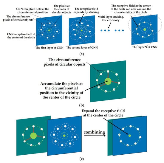 Figure 3. Schematic diagram of CNN, FGMRST/FRST, and dual-channel method applied to circular objects. (a) CNN applied to circular objects; (b) FGMRST/FRST applied to circular objects; (c) dual-channel method applied to circular objects.
 - It depends on the abundance and quantity of training samples, which does not exist in the traditional parameterized feature extraction method.
2.2. FGMRST-Based Localization Method of the Oil Tank
2.2.1. Introduction of FRST Theory
FRST is a transform that utilizes local radial symmetry to highlight points of interest within a scene [19]. The approach was inspired by the results of the generalized symmetry transform [21,22,23], although the final method bears more similarity to the work of Sela and Levine [24] and the circular Hough transform [19,25,26]. The approach presented herein determines the contribution each pixel makes to the symmetry of pixels around it, rather than considering the contribution of a local neighborhood to a central pixel [19].
The new transform is calculated at one or more radii n ∊N, where N is the set of radii of the radially symmetric features to be detected. The value of the transform at the radius n indicates the contribution to radial symmetry of the gradients a distance n away from each point.
Firstly, the positively affected pixels and the negatively affected pixels are defined: for pixel p, the positively affected pixel is defined as the pixel that the gradient vector g(p) is pointing to, a distance n away from p, and the negatively affected pixel is the pixel a distance n away that the gradient is pointing directly away from.
The coordinates of the positively affected pixel are given by:
while those of the negatively affected pixel are:
where “round” rounds each vector element to the nearest integer. The positively affected pixel and the negatively affected pixel are shown in Figure 4:
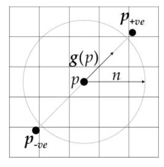
Figure 4.
Schematic map of the positively affected pixel and the negatively affected pixel.
At each radius n, an orientation projection image On and a magnitude projection image Mn are formed. For each pair of affected pixels, the corresponding point p+ve in the orientation projection image On and magnitude projection image Mn is incremented by 1 and ||g(p)||, respectively, while the point corresponding to p−ve is decremented by these same quantities in each image (the orientation and magnitude projection images are initially zero). That is:
The radial symmetry contribution at radius n is defined as the convolution
where
and
An is a two-dimensional Gaussian, α is the radial strictness parameter, and kn is a scaling factor that normalizes Mn and On across different radii.
The full transform is defined as the average of the symmetry contributions over all the radii considered:
An overview of the algorithm is shown in Figure 5 along with the key signals (images) involved.

Figure 5.
Schematic diagram of FRST.
The effect of FRST applied to the human eye is shown in Figure 6:
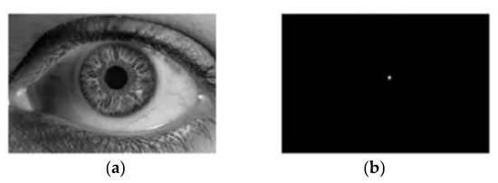
Figure 6.
FRST method is applied to the human eye. (a) Original image; (b) transformed image.
In FRST, the idea of using image gradient to localize points of high radial symmetry makes it suitable for circle detection. In addition, it does not need to traverse the whole circle as CNN does, but only needs to use the circumference and its surrounding pixels to complete the transformation (as shown in Figure 2b). Therefore, the computation complexity is low, and the runtimes are fast. The schematic diagram of the object with a circular structure is shown in Figure 3b.
2.2.2. An Improved FRST Algorithm Based on the Characteristics of Oil Tank Images—FGMRST
In this study, we conduct analyses and experiments based on the SkySat satellite with a resolution of 0.8 m.
The analysis of feature extraction using FRST in oil tank images is provided below. As shown in Figure 7, we used FRST to transform 68 × 68 images with different radii as input.

Figure 7.
Comparison of results. (a) Original image; (b) when the radius is 23.5; (c) when the radius range is [20,27]; (d) when the radius range is [1,34].
It can be seen that:
- When the floating roof of the oil tank is lower than the tank wall, there will be two areas that are brighter and darker in the image (as shown in Figure 7a), which makes positively affected pixels and negatively affected pixels at the boundary of the floating roof offset each other during transformation. Thus, the distribution of pixel values of orientation projection image and magnitude projection image is affected, and the final transformation result is affected. The solution to this problem in this study is to change the processing object of FRST from pixel to gradient modulus of pixel and cancel the positively affected pixel. Since the positively and negatively affected pixels play decisive roles in aggregating “black circle” (circle whose contour is darker than the background) and “white circle” (circle whose contour is brighter than the background), respectively, the coexistence of these two pixels makes FRST have the function of aggregating both “black circle” and “white circle” on an image. However, when the circle in the image is not a complete “black circle” or “white circle”, the coexistence of the positively and negatively affected pixels will interfere with each other, thus affecting the aggregation effect of circles. After all the pixels are processed into a gradient modulus, all circles in the image will become “white circles”, and then only negatively affected pixels need to be retained (because positively affected pixels have little effect on aggregating “white circles”), which solves the problem that some positively and negatively affected pixels offset each other during transformation.
- In the transformation results, almost only one aggregation area can be seen (see Figure 7b,c), and it is impossible to distinguish the center of the tank roof from the center of the circular-arc-shaped shadow cast by the sun on the floating roof. Therefore, FRST cannot complete the accurate localization task of the oil tank in this study. In view of the fact that the positions of the two circle centers are close, and the blur effect of the 3 × 3 Sobel operator used in FRST to calculate the gradient will have an adverse effect on accurate localizing, a simple first-order difference is used to calculate the gradient instead in this study.
- The effect of the transformation is greatly limited by the range of the input radius, and the wider the range, the worse the effect, which leads to the transformation being extremely dependent on the priori knowledge of radius. It can be inferred that the parameters related to the radius in FRST are particularly important to the result. The value of scaling factor kn is 9.9 by default when the radius is not 1, but this value is an empirical value given in an experiment with a radius range of 2–30. However, in this study and practice, the radius may exceed 30. Therefore, in this study, Mn and On are normalized by dividing all pixels in Mn and On by the maximum value of pixels in Mn and On respectively instead of kn.
In this study, the modified algorithm is named fast gradient modulus radial symmetry transform (FGMRST), and the specific transformation process is as follows:
FGMRST is calculated at one or more radii n ∊ N, where N is the set of radii of the radially symmetric features to be detected. The gradient modulus of pixel p is calculated to obtain ||g(p)||. For the convenience of subsequent expression, let:
For q, the negatively affected pixel is defined as the pixel that the gradient vector g(q) is pointing directly away from, a distance n away from q. The coordinates of the negatively affected pixel are given by:
where “round” rounds each vector element to the nearest integer. The negatively affected pixel is shown in Figure 8:
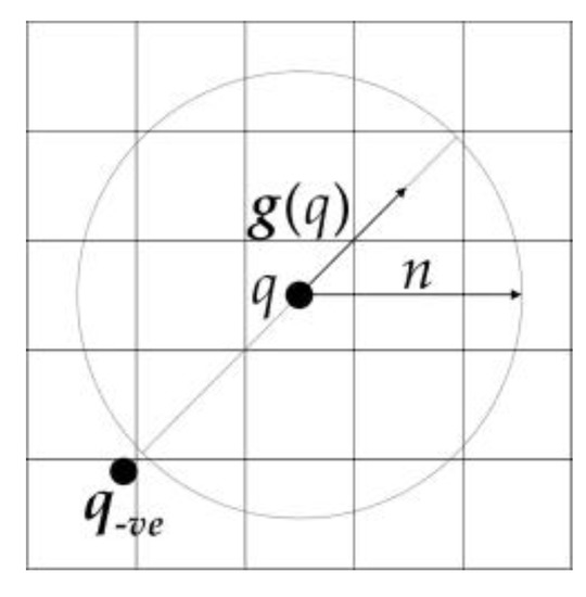
Figure 8.
Schematic map of the negatively affected pixel.
At each radius n, an orientation projection image On and a magnitude projection image Mn are formed. For each affected pixel, the corresponding point q−ve in the orientation projection image On and magnitude projection image Mn is decremented by 1 and ||g(q)|| (the orientation and magnitude projection images are initially zero). That is:
The radial symmetry contribution at radius n is defined as the convolution in Equation (7), where
An is a two-dimensional Gaussian, α is the radial strictness parameter.
The full transform is defined as the average of the symmetry contributions over all the radii considered in Equation (10).
An overview of the algorithm is shown in Figure 9 along with the key signals (images) involved.

Figure 9.
Schematic diagram of FGMRST.
The analysis of feature extraction using FGMRST in oil tank images is provided below. As shown in Figure 10, we used FGMRST to transform 68 × 68 images with different radii as input.

Figure 10.
Comparison of results. (a) Original image; (b) when the radius is 23.5; (c) when the radius range is [20,27]; (d) when the radius range is [1,34].
Comparing Figure 10b,c with Figure 7b,c, it can be found that FGMRST can better extract and distinguish the two circle centers. However, the final symmetry map is produced after combining all radial symmetry images [27]. Thus, different radii information is accumulated in the output of the transform [27]. As long as the value of input radius is a range rather than a single value, the number of pixels at certain locations and specific radii that contribute to the projection matrices is not possible to be evaluated, thus the purpose of accurately localizing the circle center and determining the radius cannot be achieved.
Based on the above analysis, it is found that FGMRST alone is difficult to achieve relatively good accuracy and a relatively high level of automation for localization of oil tank in remote sensing images. It is worth noting that FGMRST has the ability to reduce the localization range of the circle center and has good transformation results for the small radius range, so it may be combined with other methods to better achieve high-precision localization of the oil tank.
2.3. FGMRST-Based CNN Localization Method of the Oil Tank
2.3.1. Overview of Methods
FGMRST cannot accurately localize the circle center and determine the radius, but it can reduce the localization range of the circle center and realize the spatial aggregation of the circular features. In this study, FGMRST and CNN are combined to construct network parameters, and an FGMRST-based CNN method is proposed. The schematic diagram of the method is shown in Figure 3. To make the receptive field at the center of the circle contain the features of the circle, CNN must expand the receptive field through multi-layer stacking, which is inefficient, while FGMRST can accumulate the peripheral pixels near the center of the circle, and the aggregation efficiency is high. Therefore, this study attempts two combination methods: New method one (called tandem method): FGMRST is used to process the original image, and then the processed image is input into CNN. New method two (called dual-channel method): the original image and the image processed by FGMRST are combined in a dual-channel manner, and then input into CNN. The comparison of calculation location and feature processing location of three methods is shown in Table 1. The convolution operation and FGMRST can only deal with the features at the circumference and the circle center, respectively. After combining them, the new method can process the circumference feature at both the circumference and the center.

Table 1.
Comparison of three methods.
2.3.2. Flow of Methods

Figure 11.
Flow chart of tandem method.

Figure 12.
Flow chart of dual-channel method.
- 1.
- Data set preparation
The center position of the tank roof, the center position of the circular-arc-shaped shadow cast by the sun on the floating roof, and the radius of the oil tank to label, were selected and the data set was created.
- 2.
- Pre-processing
The bilinear interpolation method was used to compress the sample images to a uniform size.
- 3.
- Define CNN
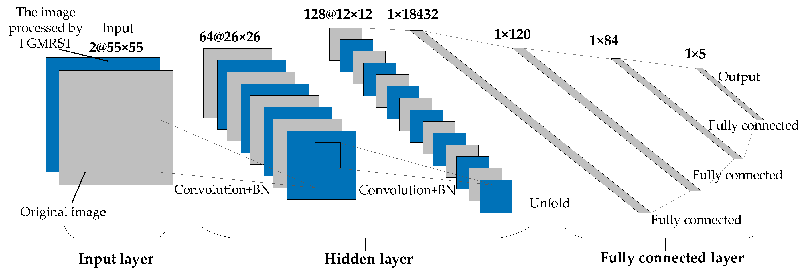
This study designed three CNN structures. The first CNN is named net_conv2, whose structure model is shown in Figure 13. It is divided into three parts: the input layer, hidden layer, and output layer. The input layer is the input sample data. The hidden layer is the key part of CNN, including two convolutional layers and two batch normalization (BN) layers. The convolutional layer is composed of a filter layer, a spatial sampling layer, and a nonlinear layer. The nonlinear layer is realized by the RELU activation function. Considering that the sampling position of the pixels for the max pooling will affect the accurate localization of the oil tank, the sampling is realized by setting the stride of two convolutional layers to 2 instead of adding the pooling layer. The output layer is a fully connected layer, which is designed as a three-layer perceptron, and the number of output features of each layer is 120, 84, and 5, respectively. After the samples are input into CNN, the hidden layer is used for feature extraction, and then the fully connected layer is used to predict the related parameters. The second CNN is named net_conv3, which adds a convolutional layer and a BN layer after the second BN layer of net_conv2, and the others remain unchanged. The structure model is shown in Figure 14. The third CNN is named net_alex because it is modified from AlexNet [16]. Its structure model is shown in Figure 15. It is also divided into three parts: input layer, hidden layer, and output layer. The hidden layer contains five convolutional layers. The convolutional layer is also composed of a filter layer, a spatial sampling layer, and a nonlinear layer. The nonlinear layer is realized by the RELU activation function. Considering that the sampling position of the pixels for the max pooling affects the accurate localization of the oil tank, the sampling is realized by setting the stride of five convolutional layers as 2, 2, 1, 2, and 2, respectively, instead of adding the pooling layer. The output layer is a fully connected layer, which is designed as a two-layer perceptron, and the number of output features of each layer is 1024 and 5, respectively.
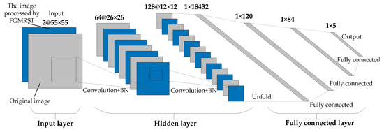
Figure 13.
Structural model of net_conv2.

Figure 14.
Structural model of net_conv3.

Figure 15.
Structural model of net_alex.
- 4.
- Training network
The L1Loss function is suitable for regression problems, so we chose it as the loss function, as shown in the following formula:
where y represents the real value and represents the output of the model.
For the consideration of convergence speed and accuracy, the Adaptive Moment Estimation (Adam) algorithm was selected to update network parameters.
The training samples were trained, the loss curve was drawn, and the training situation was judged by observing the trend of the curve.
- 5.
- Testing network on the test set
The test samples were used for testing, the average losses of each and the total of the five parameters were calculated, and the loss curve in sample units was drawn.
3. Experiments and Results
3.1. Training Details
In this study, nine experiments were designed based on the proposed method, as shown in Table 2.

Table 2.
Experimental arrangements.
3.2. Data sets
This paper uses SkySat satellite data, which is a sub-meter resolution microsatellite for business-oriented commercial earth observation [20]. The experimental data set in this paper is based on 1312 image slices fabricated from 0.8m resolution SkySat images, which is divided into 1024 training samples and 288 test samples (the proportion is close to 4:1).
3.3. Experimental Process and Results
The experiment relies on the algorithm designed in Section 2.3.2 and is carried out once each under the condition that the random seed is 0 and 1.
In the preparation before training, the learning rate of optimizer Adam is shown in Table 3. The exponential decay rate of the first moment estimation is 0.9, and that of the second moment estimation is 0.99. The MultiStepLR method was used to adjust the learning rate dynamically, setting epoch (the number of iterations) = 300 and epoch = 650 as the milestones of the learning rate, and the learning rate adjustment multiplier factor (gamma) is 0.5.

Table 3.
Total average prediction errors of five parameters in experiments.
In the training process, 1024 samples (32 batches) of the train set were used for training, and GPU was used to accelerate the training. We set epoch = 1000, then drew the loss curve, and judge the training situation by observing the trend of the curve.
In the testing process, 288 samples (9 batches) of the test set were used for testing, and then the average losses of each and the total of the five parameters were calculated on the test result. The size of the sample image was restored to the state before compression, and the predicted values of sample parameters were converted according to the same compression ratio. The converted result was used to represent the predicted values of the sample parameters under the original size, and the loss between this value and the value of the original sample was calculated. The loss curve in sample units was drawn.
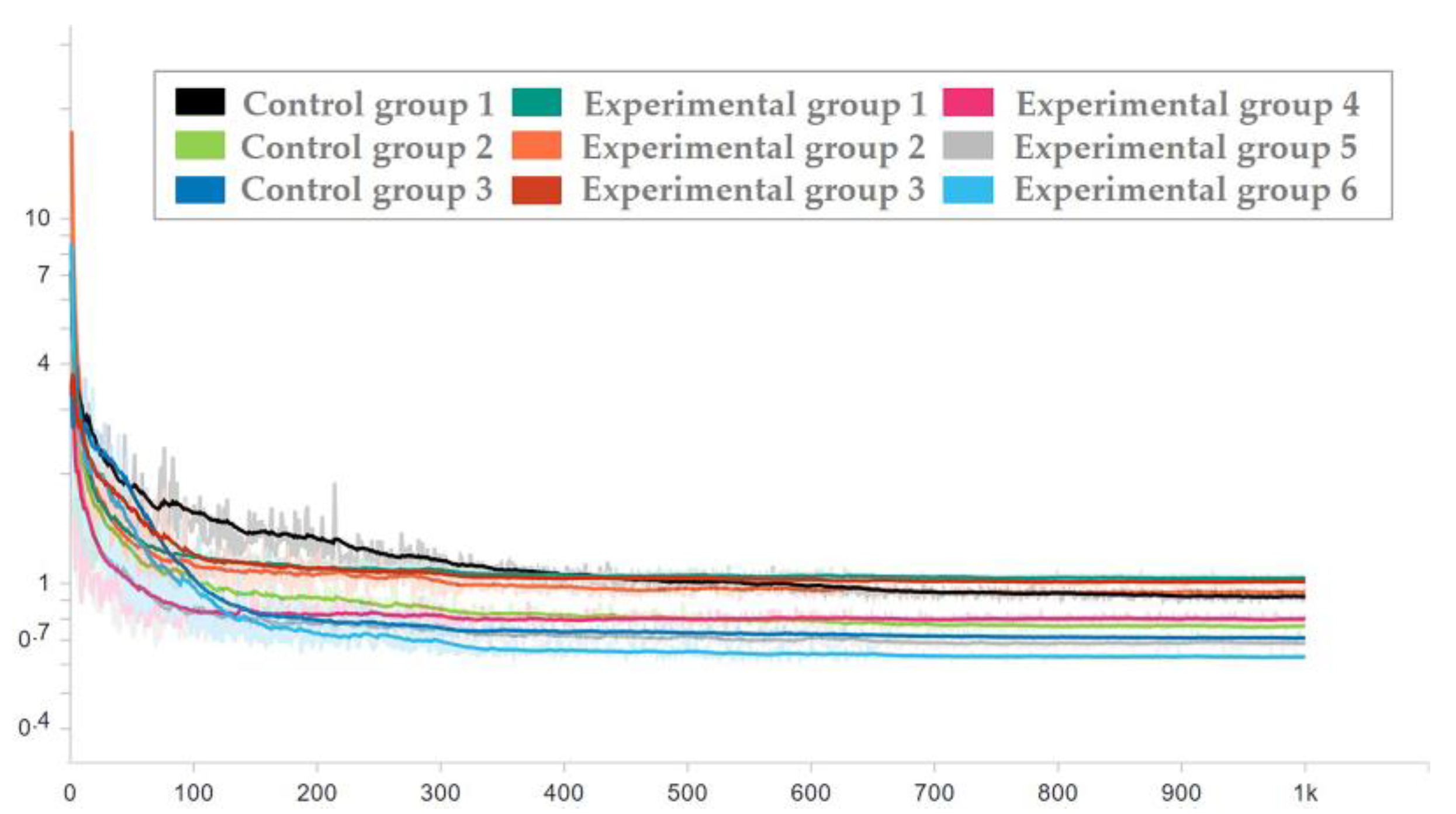
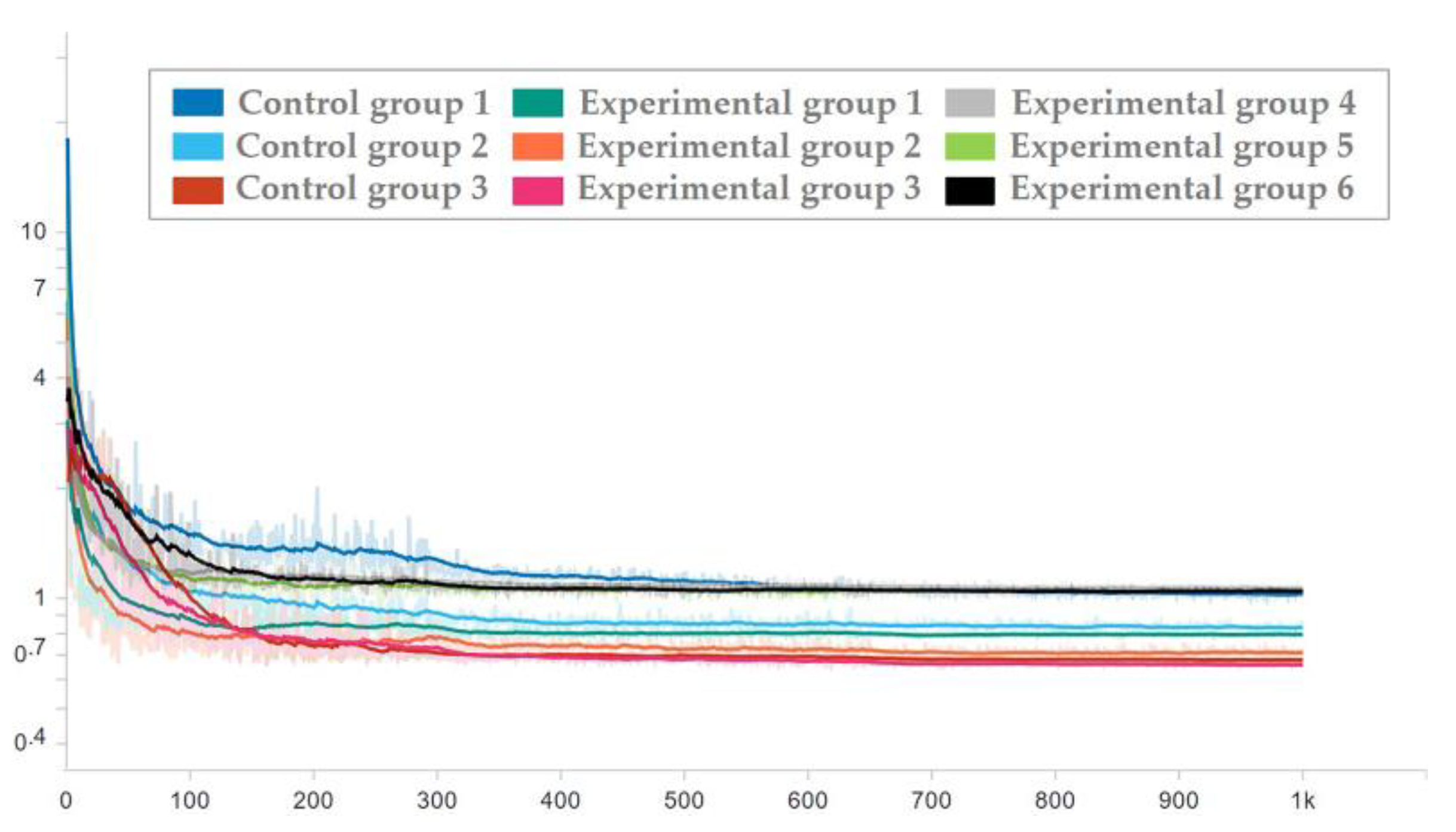
To ensure the effectiveness of the network used in the test set, the network corresponding to each epoch in the training process was applied to the test set, and the loss trend diagram of the test set is drawn as shown in Figure 16 and Figure 17. To ensure the display effect, the y-axis was logarithmic and smoothed, and the smoothing coefficient was set to 0.95.
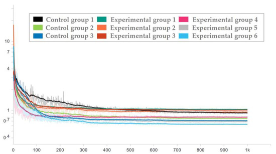
Figure 16.
Loss trend of the test set with random seed 0.
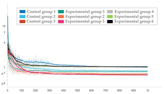
Figure 17.
Loss trend of the test set with random seed 1.
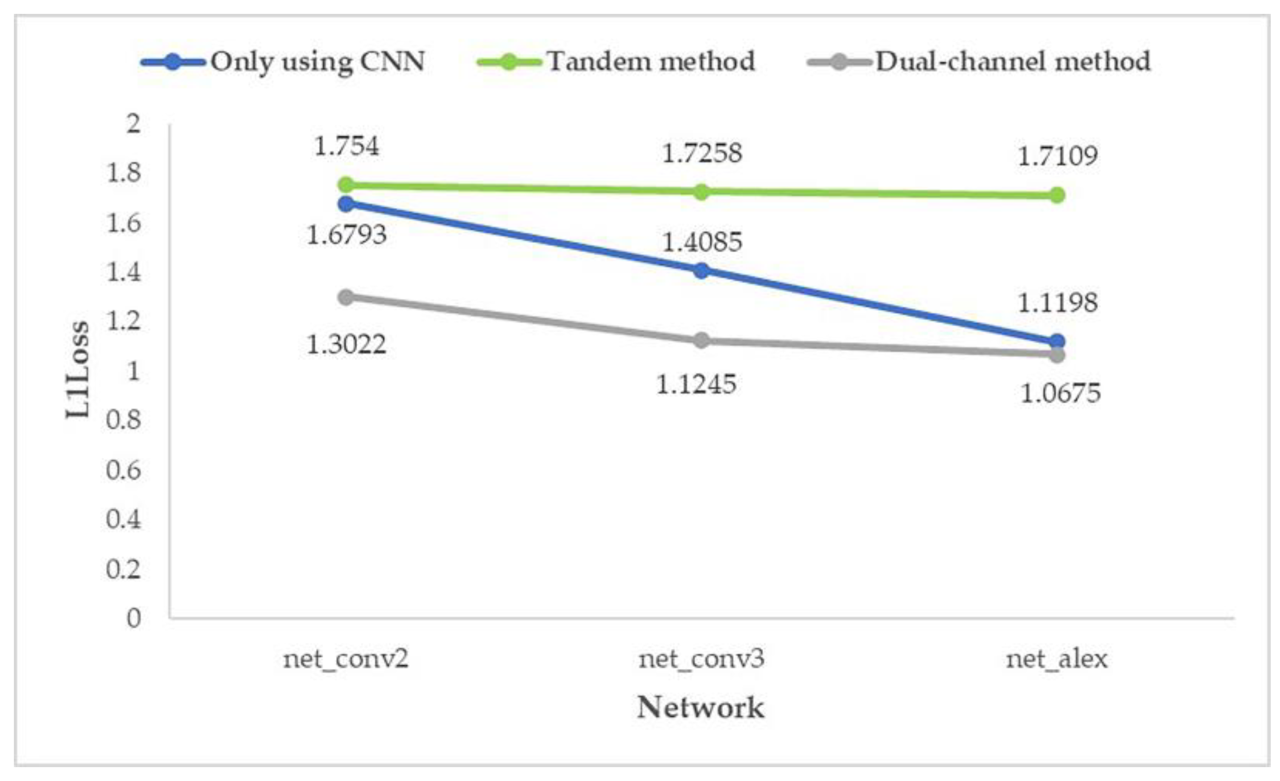
It can be seen from the figure that after the milestones of learning rate (epoch = 300 and epoch = 650), the loss is still decreasing. After the guarantee was obtained, the trained network was used to process the test set, and then the average prediction loss of five parameters was calculated on the result, as shown in Figure 18 and Figure 19.
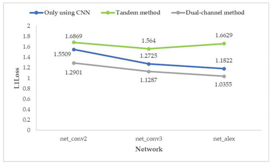
Figure 18.
Average prediction loss of five parameters with random seed 0.

Figure 19.
Average prediction loss of five parameters with random seed 1.
From the above two graphs (Figure 18 and Figure 19), it can be found that for the prediction effect, no matter what kind of structure of the network is, the “dual-channel method” better than “only using CNN” which is better than the “tandem method”; and the effect of “dual-channel method” improves with the increase in network depth.
The total average prediction errors of these nine experiments for the five parameters are provided in the following table.
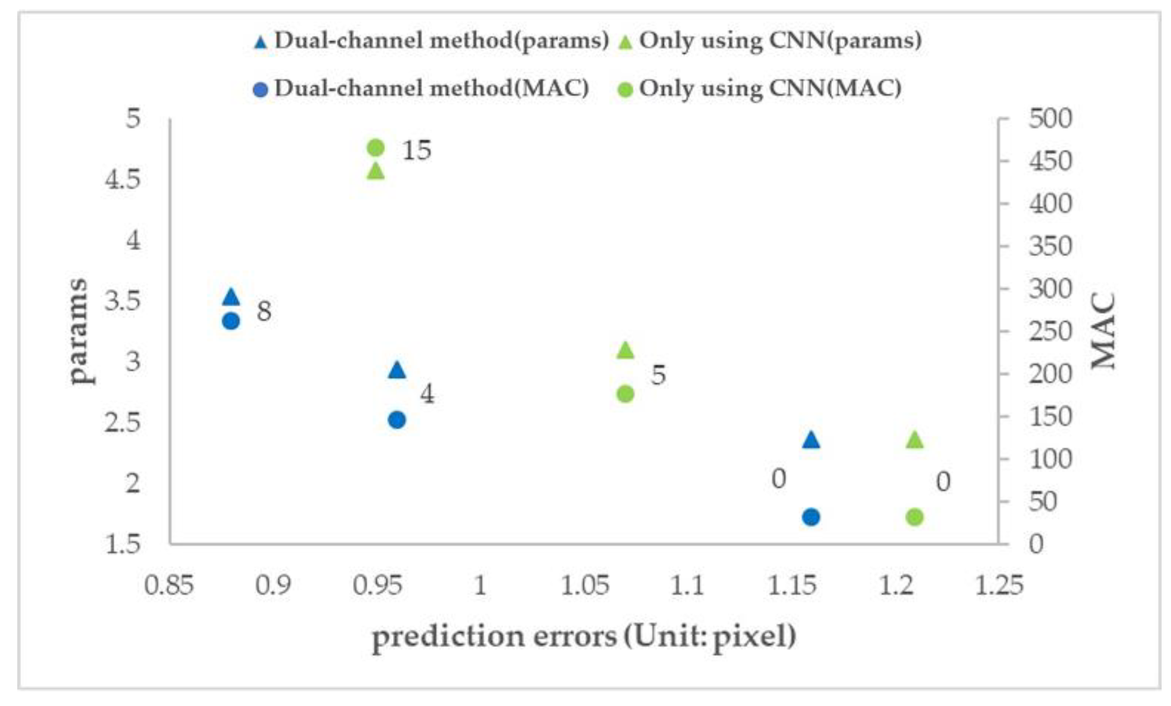
To measure the impact of the dual-channel method on computational efficiency, two physical quantities, params and multiplication and addition counts (MACs), were introduced to evaluate different network methods, as shown in Table 4. Figure 20 is drawn according to Table 4, and the data marked in the figure indicates the number of additional convolution layers added on net_conv3.

Table 4.
Prediction error and computational efficiency of different networks.
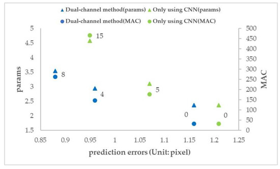
Figure 20.
Prediction error and computational efficiency of different networks.
- When the number of additional convolution layers is 0, the number of parameters and computation (params and MAC) of the two methods are the same, but the prediction error of the dual-channel method is less than that of the ordinary CNN method.
- The prediction error of adding 4 layers in the dual-channel method is close to that of adding 15 layers in the ordinary CNN method, but the amount of parameters (params) of the latter is 1.6 times that of the former, and the amount of computation (MAC) of the latter is 3.2 times that of the former.
- The number of parameters and computation (params and MAC) of the two methods increases with the increase in the number of network layers, but the dual-channel method grows more slowly. Therefore, the dual-channel method effectively reduces the number of parameters and computation, that is, improves the computational efficiency.
4. Conclusions
To improve the accuracy and stability of the localization of the oil tank in remote sensing images, this paper proposes an FGMRST-based CNN method. Experiments based on SkySat show that:
- In the FGMRST-based CNN method, the average prediction error of the dual-channel method is reduced by 14.64% compared with the ordinary CNN method, which effectively improves the accuracy.
- In the shallowest network (net_conv2), the average prediction error of the dual-channel method is reduced by 19.66% compared with the ordinary CNN method. In the deeper network (net_conv3), the average prediction error is reduced by 15.73%. In the deepest network (net_alex), the average prediction error is reduced by 8.54%. It shows that the proposed method is still better than the method using only CNN when the number of network layers increases.
- In the FGMRST-based CNN method, the dual-channel method significantly improves the computational efficiency compared with the ordinary CNN method.
The main work and innovation of this paper are as follows:
An improved FRST algorithm based on the characteristics of oil tank images is proposed, FGMRST. The advantages and disadvantages of FGMRST and CNN are discussed, and the FGMRST-based CNN method is designed, which is different from the traditional deep learning method that expends the receptive field by sacrificing resolution or increasing the model size. With only a little extra computation cost of FGMRST, the dual-channel method can efficiently aggregate spatial features, effectively improve the accuracy and stability of localization of the oil tank and improve the real-time performance in practical application.
The disadvantage of this study are as follows:
Due to the limitation of time and the author’s ability, only two combination methods of FGMRST and CNN are designed in this paper. In future work, we will continue to explore the combination of the traditional parameterized feature extraction method and the deep learning method. A key challenge in the work was the cast of shadows of the object. It was addressed using a gradient approach. However, there are still some unwanted shadows in the image (such as those caused by the uneven ground and tank top), and the method in this paper cannot eliminate the interference caused by these shadows. Therefore, in future work, we will try to combine our method with some advanced shadow detection and removal methods (such as a framework for automatic detection and removal of shadows proposed by Salman et al. [28], and methods based on paired regions proposed by Guo et al. [29,30]) to eliminate the localizing interference caused by redundant shadow information.
Author Contributions
Conceptualization, H.J., Y.Z. and J.G.; methodology, H.J.; software, H.J.; validation, H.J.; formal analysis, H.J.; investigation, H.J.; resources, H.J. and Y.Z..; data curation, H.J.; writing—original draft preparation, H.J.; writing—review and editing, H.J., Y.Z. and J.G.; visualization, H.J.; supervision, Y.Z., F.L., Y.H., B.L. and C.D.; project administration, Y.Z.; funding acquisition, Y.Z. All authors have read and agreed to the published version of the manuscript.
Funding
This work is supported by the National Key Research and Development Program of China (Grant No.2016YFF0202700) and the National Natural Science Foundation of China (Grant No.61991420).
Data Availability Statement
Not applicable.
Conflicts of Interest
The authors declare no conflict of interest.
References
- Meng, F.S. Review of change detection methods based on Remote Sensing Images. Technol. Innov. Appl. 2012, 24, 57–58. [Google Scholar]
- Sui, X.L.; Zhang, T.; Qu, Q.X. Application of Deep Learning in Target Recognition and Position in Remote Sensing Images. Technol. Innov. Appl. 2019, 34, 180–181. [Google Scholar]
- Xu, H.P.; Chen, W.; Sun, B.; Chen, Y.F.; Li, C.S. Oil tank detection in synthetic aperture radar images based on quasi-circular shadow and highlighting arcs. J. Appl. Remote Sens. 2014, 8, 397–398. [Google Scholar] [CrossRef]
- Yu, S.T. Research on Oil Tank Volume Extraction Based on High Resolution Remote Sensing Image. Master’s Thesis, Dalian Maritime University, Liaoning, China, 2019. [Google Scholar]
- Ding, W. A Practical Measurement for Oil Tank Storage. J. Lanzhou Petrochem. Polytech. 2001, 1, 4–6. [Google Scholar]
- Duda, R.O.; Hart, P.E. Use of the Hough transformation to detect lines and curves in pictures. Commun. ACM 1972, 15, 11–15. [Google Scholar] [CrossRef]
- Shin, B.G.; Park, S.Y.; Lee, J.J. Fast and robust template matching algorithm in noisy image. In Proceedings of the International Conference on Control, Automation and Systems, Seoul, Korea, 17–20 October 2007. [Google Scholar]
- Wu, X.D.; Feng, W.F.; Feng, Q.Q.; Li, R.S.; Zhao, S. Oil Tank Extraction from Remote Sensing Images Based on Visual Attention Mechanism and Hough Transform. J. Inf. Eng. Univ. 2015, 16, 503–506. [Google Scholar]
- Han, X.W.; Fu, Y.L.; Li, G. Oil Depots Recognition Based on Improved Hough Transform and Graph Search. J. Electron. Inf. Technol. 2011, 33, 66–72. [Google Scholar] [CrossRef]
- Cai, X.Y.; Sui, H.G. A Saliency Map Segmentation Oil Tank Detection Method in Remote Sensing Image. Electron. Sci. Technol. 2015, 28, 154–156, 160. [Google Scholar]
- Zhang, W.S.; Wang, C.; Zhang, H.; Wu, F.; Tang, Y.X.; Mu, X.P. An Automatic Oil Tank Detection Algorithm Based on Remote Sensing Image. J. Astronaut. 2006, 27, 1298–1301. [Google Scholar]
- Hinton, G.; Osindero, S.; Teh, Y. A Fast Learning Algorithm for Deep Belief nets. Neural. Comput. 2006, 18, 1527–1554. [Google Scholar] [CrossRef] [PubMed]
- Lecun, Y.; Bengio, Y.; Hinton, G. Deep learning. Nature 2015, 521, 436. [Google Scholar] [CrossRef] [PubMed]
- Sun, Z.J.; Xue, L.; Xu, Y.M. Overview of deep learning. Appl. Res. Comput. 2012, 29, 2806–2810. [Google Scholar]
- Lecun, Y.; Boser, B.; Denker, J.S.; Henderson, D.; Howard, R.; Hubbard, W.; Jackel, L. Backpropagation Applied to Handwritten Zip Code Recognition. Neural. Comput. 1989, 1, 541–551. [Google Scholar] [CrossRef]
- Krizhevsky, A.; Sutskever, I.; Hinton, G. ImageNet Classification with Deep Convolutional Neural Networks. In Proceedings of the Annual Conference on Neural Information Processing Systems, Lake Tahoe, NV, USA, 3–8 December 2012. [Google Scholar]
- Deep Residual Learning for Image Recognition. Available online: https://arxiv.org/pdf/1512.03385.pdf (accessed on 1 October 2020).
- Wang, Y.J.; Zhang, Q.; Zhang, Y.M.; Meng, Y.; Guo, W. Oil Tank Detection from Remote Sensing Images based on Deep Convolutional Neural Network. Remote Sens. Technol. Appl. 2019, 34, 727–735. [Google Scholar]
- Loy, G.; Zelinsky, A. Fast radial symmetry for detecting points of interest. IEEE Trans. Pattern Anal. Mach. Intell 2003, 25, 959–973. [Google Scholar] [CrossRef] [Green Version]
- Gong, R. Sky Sat. Satell. Appl. 2016, 7, 82. [Google Scholar]
- Reisfeld, D.; Wolfson, H.; Yeshurun, Y. Context-free attentional operators: The generalized symmetry transform. Int. J. Comput. Vis. 1995, 14, 119–130. [Google Scholar] [CrossRef]
- Intrator, N.; Reisfeld, D.; Yeshurun, Y. Extraction of Facial Features for Recognition using Neural Networks. Acta Obs. Gynecol Scand. 1995, 19, 1–167. [Google Scholar]
- Reisfeld, D.; Yeshurun, Y. Preprocessing of Face Images: Detection of Features and Pose Normalization. Comput. Vis. Image Underst. 1998, 71, 413–430. [Google Scholar] [CrossRef]
- Sela, G.; Levine, M.D. Real-Time Attention for Robotic Vision. Real-Time Imaging 1997, 3, 173–194. [Google Scholar] [CrossRef] [Green Version]
- Kimme, C.; Balard, D.; Sklansky, J. Finding Circles by an Array of Accumulators. Commun. ACM 1975, 18, 120–122. [Google Scholar] [CrossRef]
- Minor, L.G.; Sklansky, J. The Detection and Segmentation of Blobs in Infrared Images. IEEE Trans. Syst. Man Cybern. 1981, 11, 194–201. [Google Scholar] [CrossRef]
- Ok, A.O.; Baseski, E. Circular Oil Tank Detection from Panchromatic Satellite Images: A New Automated Approach. IEEE Geosci. Remote Sens. Lett. 2015, 12, 1347–1351. [Google Scholar] [CrossRef]
- Khan, S.H.; Bennamoun, M.; Sohel, F.; Togneri, R. Automatic Shadow Detection and Removal from a Single Image. IEEE Trans. Pattern Anal. Mach. Intell 2016, 38, 431–446. [Google Scholar] [CrossRef] [PubMed] [Green Version]
- Guo, R.Q.; Dai, Q.Y.; Hoiem, D. Paired Regions for Shadow Detection and Removal. IEEE Trans. Pattern Anal. Mach. Intell 2013, 35, 2956–2967. [Google Scholar] [CrossRef] [PubMed]
- Guo, R.Q.; Dai, Q.Y.; Hoiem, D. Single-image shadow detection and removal using paired regions. In Proceedings of the IEEE Conference on Computer Vision and Pattern Recognition, Colorado Springs, CO, USA, 20–25 June 2011. [Google Scholar]
Publisher’s Note: MDPI stays neutral with regard to jurisdictional claims in published maps and institutional affiliations. |
© 2021 by the authors. Licensee MDPI, Basel, Switzerland. This article is an open access article distributed under the terms and conditions of the Creative Commons Attribution (CC BY) license (https://creativecommons.org/licenses/by/4.0/).

