Error Characteristics of Pan-Arctic Digital Elevation Models and Elevation Derivatives in Northern Sweden

Abstract

Many biochemical processes and dynamics are strongly controlled by terrain topography, making digital elevation models (DEM) a fundamental dataset for a range of applications. This study investigates the quality of four pan-Arctic DEMs (Arctic DEM, ASTER DEM, ALOS DEM and Copernicus DEM) within the Kalix River watershed in northern Sweden, with the aim of informing users about the quality when comparing these DEMs. The quality assessment focuses on both the vertical accuracy of the DEMs and their abilities to model two fundamental elevation derivatives, including topographic wetness index (TWI) and landform classification. Our results show that the vertical accuracy is relatively high for Arctic DEM, ALOS and Copernicus and in our study area was slightly better than those reported in official validation results. Vertical errors are mainly caused by tree cover characteristics and terrain slope. On the other hand, the high vertical accuracy does not translate directly into high quality elevation derivatives, such as TWI and landform classes, as shown by the large errors in TWI and landform classification for all four candidate DEMs. Copernicus produced elevation derivatives with results most similar to those from the reference DEM, but the errors are still relatively high, with large underestimation of TWI in land cover classes with a high likelihood of being wet. Overall, the Copernicus DEM produced the most accurate elevation derivatives, followed by slightly lower accuracies from Arctic DEM and ALOS, and the least accurate being ASTER.

1. Introduction

Topography is a fundamental property of the terrain that strongly influences a large number of biogeochemical processes and dynamics that take place on the Earth’s surface [1]. Consequently, digital elevation models (DEMs) are key datasets for studying and modelling Earth surface features and processes, of relevance for hydrology, agronomy, geomorphology, soil formation and land cover mapping [2]. A DEM is a digital representation of a terrain surface usually conceptualised as a grid, where the grid-cell values represent the elevation of a specific area relative to a reference value (e.g., sea level). At present, differences exist in the terminology and definitions concerning DEMs, as well as the associated terms digital surface model (DSM) and digital terrain model (DTM) [3,4,5]. The term DEM is used here as a general umbrella term for all types of elevation models, while the term DTM refers to the model representing the elevation of the bare ground, and the term DSM refers to the model representing the elevation, which includes any natural and manmade features located on the Earth surface [5,6]. In other words, DTMs are a bare-Earth model, where heights of natural or manmade features, if present, have been removed.

The recent progress in satellite remote sensing technology has paved the way to produce several global or regional DEMs with increasing accuracy and spatial resolution. Widely used products include Shuttle Radar Topography Mission (SRTM) [7], Advanced Spaceborne Thermal Emission and Reflection Radiometer (ASTER) Global DEM [8], Advanced Land Observing Satellite (ALOS) World 3D [9] and TanDEM-X WorldDEM^TM [10,11]. These are all examples of DEMs with medium spatial resolution (30–100 m cell size) that are freely available to the user community. Such wide-area coverage DEMs are of high value in areas where national mapping agencies or other actors have not created higher spatial resolution products based on Light Detection and Ranging (LiDAR) or aerial photogrammetry [12]. In addition, these products provide seamless and consistent data coverage beneficial for large area applications, such as regional scale hydrological modelling and land cover mapping [13,14]. The main difference between these wide-area coverage products is the techniques used for data acquisition and processing of the raw signal to DEM, which influence their respective properties and qualities. For example, SRTM and TanDEM-X were produced from synthetic aperture radar (SAR) acquisitions, whereas ASTER and ALOS are based on photogrammetric processing of optical imagery.

Information about topography, including forms and features of the land surface, is of particular importance in the Arctic (>60 °N), which is a geographical region that has experienced large effects of global climate change with increasing land surface temperature and changes in precipitation patterns [15,16]. The availability of accurate DEM information is key for studying and monitoring environmental processes and responses related to the climate and its dynamics, including land surface warming, permafrost thaw, thermokarst development, as well as changes in vegetation cover and the impacts on biogeochemical cycles [17,18,19]. In addition, DEMs are also crucial for rectification of other remote sensing data, including compensating for diverse incidence and sun elevation angles [20]. Previously, wide-area coverage DEMs have had incomplete coverage or significant data gaps in the Arctic because of limitations mainly related to the satellite systems used for data acquisition and environmental conditions. However, the last few years have seen the release of several DEMs with pan-Arctic coverage and a spatial resolution of 30 m or less. This includes improved versions of ALOS World 3D (v. 3.1 in 2020) and ASTER (v. 3 in 2019), Arctic DEM (v. 3.0 in 2018) and Copernicus DEM (v. 1 in 2020).

Given the high applicability of DEMs, it is important to assess their accuracy in order to understand their respective qualities, capabilities and limitations [21]. This is also the focus of the recently launched initiative, called the Digital Elevation Model Intercomparison Experiment (DEMIX), which targets global DEM benchmarking [22]. The vertical accuracy of a DEM, or its ability to represent the true elevation, is a key consideration when selecting between different DEMs for a particular application. The accuracy of a DEM is usually quantified through comparison with a data source of higher quality and resolution, such as elevation records from global navigation satellite systems, topographic maps, ground surveys and aerial LiDAR acquisitions [21]. An alternative approach to DEM accuracy assessment is to use vertical profiles of paved runways characterised by flatness and homogenous material as reference data, against which comparisons are made [23,24]. A general approximation of the vertical accuracy is usually provided in the metadata of a DEM product. However, from an application perspective, more relevant aspects of DEM accuracy are related to the applicability, or “fitness for use”, of a DEM [25]. Assessments of DEM applicability can both focus on specific geographical regions or terrain types [26,27,28], as well as the ability of a DEM to model secondary elevation derivatives with applications in, for example, hydrology and geomorphology [29,30,31,32]. The data acquisition technique used to create the DEM is one of the main determinants of the vertical accuracy, but the terrain characteristics of the area of interest also play an important role [21]. In addition, accuracy of a DEM can differ spatially depending on land cover characteristics and dynamics, including the influence of tree cover and land surface conditions (e.g., soil moisture and snow cover) [33].

While the evaluation of wide-area coverage DEMs has been the focus of numerous studies, only a few of them have targeted Arctic areas. In a recent study, Glennie (2018) assessed several high-resolution DEMs generated from interferometric SAR, as well as three versions of Arctic DEM over a 25-km² area centred on Sitka, Alaska [33]. The mean vertical error of the Arctic DEM products ranged between 8.07–15.75 m when elevation was compared with reference datasets produced from airborne LiDAR acquisitions. Arctic DEM performed best in areas with little or no vegetation and in relatively flat areas. Xing et al. (2020) compared four DEMs over Greenland, including two from the Greenland Ice Mapping Project (GIMP), TanDEM-X and ArcticDEM [34]. The GIMP DEMs are combinations of several regional DEMs and ASTER DEM with the processing workflow outlined in [35]. Xing et al. (2020) concluded that TanDEM-X performed best in terms of both vertical accuracy (RMSE 5.6 m) and applicability, in this case for the automatic extraction of river network information in Greenland. Toutin et al. (2013) described the production and evaluation of a DEM produced from RADARSAT-2 imagery covering a coastal area in Nunavut close to Baffin Island, northern Canada [36]. Similar to many other studies, these authors observed that elevation error is often a function of increasing slope [36]. Consequently, previous studies evaluating the quality of pan-Arctic DEMs are limited in number, as well as geographical scope, considering the large extent of the region and the high diversity in topography and land cover conditions. In addition, key qualitative aspects of the most recent versions of pan-Arctic DEMs have not been reported. This includes both vertical accuracy and abilities to model fundamental elevation derivatives, such as upstream area, local slope and landform classes in key Artic land cover types, such as tundra, wetlands and forests.

The aim of this study is to analyse the quality of four recently released DEMs with pan-Arctic coverage, including ASTER DEM, ALOS World 3D, Arctic DEM and Copernicus DEM, in the Kalix River watershed located in the Arctic region of Sweden. This is achieved by comparing these four candidate DEMs with a LiDAR-based, high-spatial resolution DTM produced by the Swedish Mapping, Cadastral and Land Registration Authority, which is considered here to represent the true elevation of the bare Earth surface. Our accuracy assessment considers both vertical accuracy, as well as the applicability of the candidate DEMs to model two elevation derivatives, including topographic wetness index (TWI) and landform classification. We assess both the overall accuracy of the candidate DEMs, the spatial variation of vertical error, as well as accuracies in specific land cover categories.

2. Study Area and Data

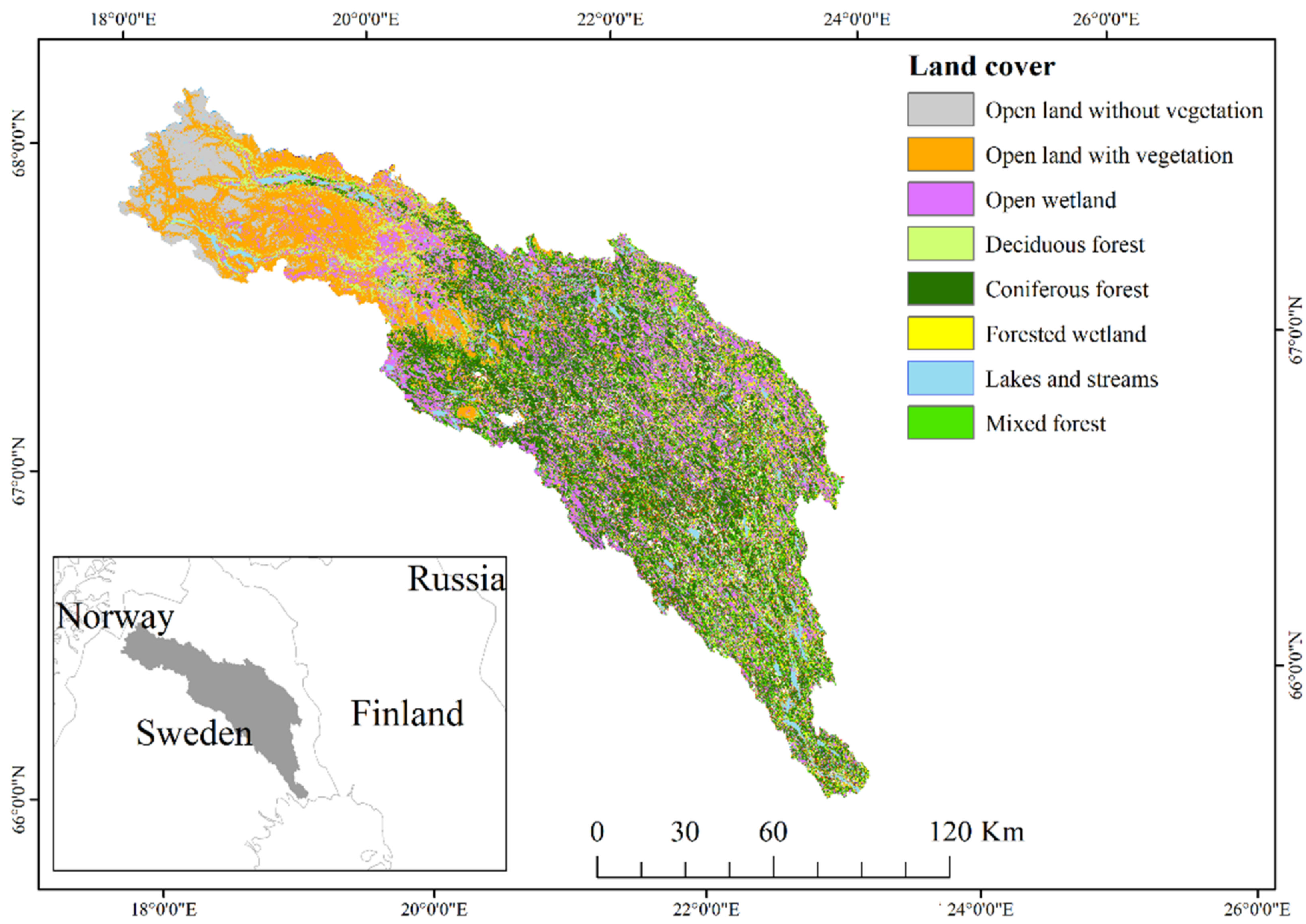
2.1. Study Area

The Kalix River watershed is located in the most northern parts of Sweden and encompasses an area of 18,122 km² (Figure 1). This is a sparsely populated watershed, with Kiruna as the largest city (pop. 16 420 in 2018). The main land cover classes include forest (63%, of which 79% is coniferous and 21% deciduous), wetland (18%), open land (13%) and inland water (4%) [37]. Kalix River is one of Sweden’s four untouched rivers where no hydropower has been installed. The river is 430 km long, flows southeast from the origin in the mountainous region near the border with Norway, and ends in the Bothnian Bay southeast of the city of Kalix. The elevation in the watershed ranges between 0–2096 m above sea level. This study area was chosen because it represents land cover conditions that apply over large parts of the Arctic and is characterised by high spatial variability in topography, including both mountains, foothills, valleys and plains.

The National Land Cover data includes data on vegetation height classes derived from the airborne LiDAR data provided by the Swedish Mapping, Cadastral and Land Registration Authority. The distribution of vegetation height classes is provided in

Table 1. Distribution of vegetation height classes over all land cover classes except water bodies in the Kalix River watershed.

Distribution of Vegetation Height Classes in Study Area
Height class (m)	0–0.5	0.5–5	5–10	10–15	15–20	20–25	>25–30
Percent of study area	29.1%	15.4%	30.5%	19.2%	5.4%	0.3%	<0.1%
Total area (km2)	5277	2790	5536	3487	986	50	1

for the purpose of describing the vegetation in the study area that might have an influence on DSMs.

2.2. Data

2.2.1. Arctic DEM

Arctic DEM is a DSM that covers the regions above 60 °N latitude and is the outcome of a partnership between the National Science Foundation, the National Geospatial-Intelligence Agency and Digital Globe Inc. [38]. The DSM was created using autocorrelation techniques on overlapping image pairs, primarily from the Digital Globe constellation of optical satellites, including ~0.5 m grid cell resolution images from WorldView-1, -2 and -3. This autocorrelation approach is called SETSM (surface extraction with TIN-based search-space minimization) [39]. A drawback of Arctic DEM is that it does include data voids, or holes, mainly due to clouds, fog, shadows or dust. Additional voids over homogeneous terrain and open water can also occur due to errors in the autocorrelation processing. The original spatial resolution of Arctic DEM is 2 m, but reduced resolution products are also available, including 10 m, 32 m, 100 m, 500 m and 1000 m products. We used the 10 m mosaicked product (version 3.0, release 7) in this study with an overall vertical RMSE of 4 m suggested by the developers [38]. Each DEM product is derived from a TIN-based model where pixels are assigned elevation values when the TIN is translated into a raster format. The 10 m product was chosen because it represents a compromise between spatial detail and data load when considering regional scale DEM application. In addition, aggregating the 2 m reference DEM to 10 m instead of 30 m to allow comparisons with the other DEMs in this study results in reduced interpolation errors [33,40]. Additional documentation about Arctic DEM is available on the Polar Geospatial Centre website hosted by the University of Minnesota (http://www.pgc.umn.edu/arcticdem; accessed on 2 September 2021).

2.2.2. ALOS World 3D 30

ALOS World 3D 30 is a DSM created by Japan Aerospace Exploration Agency (JAXA) from optical imagery collected between 2006–2011 by the Panchromatic Instrument for Stereo Mapping (PRISM) on-board the Advanced Land Observing Satellite (ALOS). DSM generation is based on matching triplets of stereoscopic images producing a commercial product with 5 m spatial resolution and a reported vertical accuracy of 5 m [41,42,43]. A resampled version of the 5 m commercial product is also available at 30 m spatial resolution. Specifically, pixel values of the 30 m product are derived from a resampling method where pixels from the 5 m product have been averaged within a 7 × 7 pixel neighbourhood [9]. We used the 30 m version 3.1 product, released in April 2020, which was done to improve the DSM quality in areas > 60 °N latitude. Additional details about ALOS World 3D are available on the JAXA website (https://www.eorc.jaxa.jp/ALOS/en/index_e.htm; accessed on 5 September 2021).

2.2.3. ASTER Global DEM

The ASTER DEM is a DSM created from optical stereo imagery acquired by the Advanced Spaceborne Thermal Emission and Reflection Radiometer (ASTER) on-board the TERRA satellite. The first version of the ASTER global DEM was released in 2009. This was a joint project between the National Aeronautics and Space Administration (NASA) and the Japanese Ministry of Economy, Trade and Economics. The most recent version (v3, or ASTER GDEM3) of this DSM was released in August 2019 with improvements in coverage and accuracy, as well as reductions of data voids and artefacts [44]. The data have a 1-arc second (ca 30 m) grid cell resolution, and the reported vertical accuracy of ASTER GDEM2 is 8.68 m RMSE [8]. Additional detail about the ASTER global DEM can be retrieved from the Jet Propulsion Laboratory website (https://asterweb.jpl.nasa.gov/gdem.asp; accessed on 5 September 2021).

2.2.4. Copernicus DEM

The Copernicus DEM product (version 2.1) is a DSM derived from an edited version of WorldDEM^TM product (ESA 2020), which was produced from radar data acquired by the TanDEM-X system. The TanDEM-X mission was operated by the German Aerospace Centre and Airbus between 2010–2015 and consisted of two similar satellites, including TerraSAR-X and TerraSAR-X add-on for Digital Elevation Measurements [10,11]. These satellites acquire SAR data in an instrument configuration that enabled dynamic, along-track, single-pass interferometry. The Copernicus DEM is available in two versions with global coverage (30 m and 90 m) and a 10 m version that covers EU-member states and their overseas territories. The 30 m global product released in 2020 was used in this study. The overall vertical and horizontal accuracies are reported to <4 m and <6 m, respectively. The 30 m product (also called “GLO-30”) has been interpolated from the highest resolution data using a weighted aggregation approach. Further details about Copernicus DEM are available at the Eurostat webpage (https://ec.europa.eu/eurostat/web/gisco/geodata/reference-data/elevation/copernicus-dem; accessed on 5 September 2021).

2.2.5. Swedish National DEM

The Swedish National DEM is a DTM produced by the Swedish Mapping, Cadastral and Land Registration Authority using aerial LiDAR data collected between 2009 and 2019, depending on geographic location, and is continuously updated. The DTM was generated from a point cloud with a density of 0.5–1 points m⁻², resulting in a product with grid cell resolution of 2 × 2 m and a horizontal and vertical error of 0.1 m and 0.3 m, respectively [45]. Objects not belonging to the Earth’s surface, including buildings and vegetation, were filtered out to produce the final DTM product. We used the Swedish National DEM as reference data against which the four candidate DEMs were compared. This reference dataset fulfils the standard requirements that the vertical accuracy of the reference should be at least three times higher than the candidate DEMs included in a comparative analysis [46].

2.2.6. Land Cover

We used the Swedish National Land Cover data released in July 2020 [37] to stratify the study area (Figure 1). This stratification enabled the assessment of how different land cover types affected candidate DEM accuracy. This product is primarily generated from the same LiDAR data described in Section 2.2.5 and Sentinel-2 imagery from 2015–2018. The horizontal accuracy is below 10 m and the classification accuracy is between 70% and 100%, depending on the specific land cover class [47]. The original product consists of 21 thematic classes in the Kalix River watershed. We excluded some classes with limited spatial extent and relevance from the land cover map in this study, including different types of developed land, ocean and agricultural land. The class called “temporary non-forest”, delimiting areas of forest regrowth, was also excluded due to it temporally dynamic nature and the difficulty to ensure consistency with the DEM products. In addition, tree species classes were aggregated to two tree type classes (coniferous and deciduous). This procedure was done for both regular forest areas and forests on wetland, resulting in eight land cover classes: open wetland (OW), open land with vegetation (OLwV), coniferous forest (CF), mixed forest (MF), deciduous forest (DF), forested wetland (FW), open land without vegetation (OloV), and lakes and streams (LK).

We also used the vegetation heights layer (Table 1) included in the land cover data to calculate mean heights of the eight land cover classes. More details about characteristics of the land cover classes, including mean and standard deviation of vegetation height, can be found in Supplementary Table S1. The land cover data can be accessed through the Swedish Environmental Protection Agency webpage (https://www.naturvardsverket.se/verktyg-och-tjanster/kartor-och-karttjanster/nationella-marktackedata; accessed on 5 September 2021).

3. Methods

3.1. Pre-Processing of DEMs

ALOS and ASTER elevations correspond to orthometric heights referenced to the EGM96 geoid, while Copernicus is referenced to the EGM2008 geoid. The reference DEM uses the national vertical reference system RH and corresponds to orthometric height referenced to the SWEN17_RH2000 geoid. The difference between these three geoids (EGM96, EGM2008 and SWEN17_RH2000) was deemed negligible in the study area and height conversions were not done for ALOS, ASTER, Copernicus and the reference DEM. On the other hand, Arctic DEM elevation corresponds to ellipsoidal heights referenced to the WGS84 ellipsoid and consequently needed conversion to orthometric height. This was achieved by subtracting the EGM96 geoid separation from the ellipsoidal height of Arctic DEM. The geoid separation was calculated by evaluating EGM96 in the study area at 0.5 degree intervals using the method outlined in the GeographicLib library [48].

The 2 m reference DEM and all 30 m candidate DEMs, except Arctic DEM, were then re-projected to the National Snow and Ice Data Centre (NSIDC) Polar Stereographic North coordinate system (EPSG:3413) and resampled to a common grid consisting of 10 × 10 m cells using bilinear interpolation. These resampled DEMs were used to derive elevation derivatives and formed the material for the comparison. The reference DEM originally had a 2 m grid cell; comparing grid cells which are an aggregation of higher resolution data to grid cells from DEMs, which originally had coarser spatial resolutions, does not result in linear comparisons. However, this process does allow the relative comparison among the DEMs tested here.

When comparing multiple DEMs and elevation derivatives, it is important that the horizontal location between them, as well as with the reference DEM, is matching. All candidate DEMs have officially reported horizontal accuracies well below the spatial resolution of the original DEM products, including <4 m for Arctic DEM [33,38], <5 m for ALOS [9], <6 m for ASTER [8,49] and <6 m for Copernicus [50]. The horizontal matching between the candidate DEMs and the reference DEM was controlled visually by comparing the locational fit of a sample of clearly identifiable objects and features distributed throughout the study area, such as waterbodies, roads and streambeds [51]. This visual assessment revealed that the officially reported horizontal accuracies of all candidate DEMs seemed reasonable and that no further co-registration was necessary. Lastly, we considered negative elevation values in all DEMs to be errors and therefore converted those pixels to no data to avoid spurious results in the comparisons.

3.2. Computation of Topographic Wetness Index

The Topographic Wetness Index (TWI; Equation (1)), first introduced by [52], is one of the most widely used hydrological-based indices that quantifies the propensity of a grid cell in a DEM to accumulate water [53]. This index is calculated as follows:

TWI = ln(α/tan(β))

(1)

where α represents the upslope catchment area that drains through a specific point, or the tendency of a location to receive water, whereas tan(β) is the local slope angle representing the propensity of a location for local runoff. We used the r.watershed package available in Geographic Resource Analysis Support System (GRASS 7.6.1), developed by the U.S. Army Corps of Engineers [54], and the multiple flow direction algorithm [55,56] to derive TWI layers from all DEMs.

3.3. Landform Classification

Landform classification is a conceptual approach to identify and delineate geomorphic or terrain features of the Earth’s surface, such as plains, valleys and plateaus. Landform information is often useful for predicting biogeochemical conditions that exist and processes that operate in a particular area. Many different methods for landform classification exist, but most are based on spatial and contextual properties of a location, such as shape, size, relief and relative position in the terrain [57].

We used the GRASS tool r.geomorphon [58] to classify all DEMs into landform maps. The relative elevation of each cell in a DEM is characterised through a comparison with at least eight neighbouring cells using a three-value scale (higher, lower, same) that represent differences in elevation values. This process generates a pattern of a visibility neighbourhood, and then labels each cell to one of 498 potential patterns, or so-called morphons. A look-up table is then used to assign each cell to one out of ten commonly recognizable landforms (

Table 2. Landform classes derived from the GRASS GIS package r.geomorphon.

Landform Class	Description
Flat	Areas with small variations in elevation and low slope
Summit	Mountain tops
Ridge	Narrow range of hills
Shoulder	Part of a hill where it curves towards the top
Spur	Lateral ridge or tongue of land descending from a hill
Slope	Areas with uniform slope
Hollow	Cavity within higher elevation areas
Footslope	Area with gently inclined slope at the foot of a hill
Valley	Long depression in the land surface that often contains a watercourse at the bottom
Depression	Area with lower elevation compared to the surrounding, but more extensive compared to a hollow

).

The r.geomorphon tool requires two scalar parameters as input: lookup distance L and flatness threshold t. Lookup distance L controls the length in number of cells where line-of-sight is calculated for producing the visibility neighbourhood and influences the size of landforms that can be detected. We set L to 9 and t to the default value 1. The selection of L and t was done by visually comparing the landform maps resulting from using multiple scalar parameter combinations to a shaded relief of the reference DEM in which common landforms are easily identifiable.

3.4. DEM Comparison and Accuracy Assessment

3.4.1. Spatial Sampling

To assess the differences between each candidate DEM and the reference DEM for elevation and TWI, all cells were used. However, cells with difference values greater than three standard deviations from the initial mean value were removed from the statistics computation to mitigate the effect of outliers [33]. These outliers were primarily artefacts located on the edges of the study area that were a result of differences in spatial resolution of the reference and candidate DEMs, as well as the resampling procedure. Difference statistics for elevation and TWI were derived both overall for each DEM comparison and for each of the eight land cover classes.

The level of agreement in elevation and TWI values between the candidate DEMs and reference DEM was computed from a subset of 220,000 cells distributed randomly throughout the study area. This subset of cells was also used to correlate errors in elevation and TWI with terrain slope derived from the reference DEM, as well as to assess the landform classification accuracy.

3.4.2. Land Cover Stratification

In addition to the overall comparison between candidate DEM and the reference DEM, difference statistics for elevation and TWI were also calculated using cells constrained by the eight land cover categories (see Section 2.2.6). This step provides land cover specific accuracies and facilitates interpretations of results from the DEM comparison. Detailed descriptions of the eight land cover classes, including vegetation height statistics, are provided in Supplementary Table S1.

3.4.3. Quality Metrics

We used several different quality metrics to assess the vertical accuracy of the candidate DEM, as well as their suitability to produce TWI, by comparison with the reference DEM. The same quality metrics were used to assess the land cover specific accuracies and included mean error (ME; bias; Equation (2)), standard deviation of error (SE; Equation (3)) and root-mean-square error (RMSE; Equation (4)). The Pearson product-moment correlation coefficient (r; Equation (5)) was used to determine the level of agreement or goodness of fit, between the candidate DEMs and reference DEM and to assess the relationship between candidate DEM error and local slope. The calculations of the quality metrics for assessing vertical and TWI accuracy are as follows:

$$\mathrm{ME}=\frac{\sum {}_{\mathit{i}=\mathit{i}}^{\mathit{n}}\left({\mathit{x}}_{\mathit{i}}-{\mathit{y}}_{\mathit{i}}\right)}{\mathit{n}}$$

(2)

$$\mathrm{SE}=\sqrt{\frac{\sum {}_{\mathit{i}=\mathit{i}}^{\mathit{n}}{({\mathit{x}}_{\mathit{i}}-{\mathit{y}}_{\mathit{i}}-\mathit{M}\mathit{E})}^{\mathbf{2}}}{\mathit{n}-\mathbf{1}}}$$

(3)

$$\mathrm{RMSE}=\sqrt{\frac{\sum {}_{\mathit{i}=\mathbf{0}}^{\mathit{n}}{({\mathit{x}}_{\mathit{i}}-{\mathit{y}}_{\mathit{i}})}^{\mathbf{2}}}{\mathit{n}-\mathbf{1}}}$$

(4)

$$\mathit{r}=\frac{\mathit{n}\left(\sum \mathit{z}\mathit{s}\right)-\left(\sum \mathit{z}\right)\left(\sum \mathit{s}\right)}{\sqrt{[\mathit{n}}\sum {\mathit{z}}^{\mathbf{2}}-{(\sum \mathit{z})}^{\mathbf{2}}\left]\right[\mathit{n}\sum {\mathit{s}}^{\mathbf{2}}-{(\sum \mathit{s})}^2]}$$

(5)

where x is the value of candidate DEMs, y is the value of reference DEM, z is the error of candidate DEM, s is the slope derived from reference DEM, while I represents the ith cell and n is the total number of cells in a DEM.

The applicability of the candidate DEMs for landform classification was assessed through the computation of a confusion matrix and the associated quality metrics’ overall accuracy (OA), producer’s accuracy (PA) and user’s accuracy (UA). OA is the proportion of correctly classified cells in a candidate DEM, whereas PA and UA are class specific metrics. PA is the proportion of correctly classified cells relative to the total number of cells in a specific class, whereas UA is the proportion of correctly classified cells relative to the total number of cells assigned to a specific class in the landform map. In addition, Cohen’s kappa coefficient (k; Equation (6)) quantifies the level of agreement between two classifications by taking into account the possibility of the agreement taking place by chance [59]. The calculation of k is as follows:

$$\mathit{k}=\frac{{\mathit{p}}_{\mathit{o}}-{\mathit{p}}_{\mathit{e}}}{\mathbf{1}-{\mathit{p}}_{\mathit{e}}}=\mathbf{1}-\frac{\mathbf{1}-{\mathit{p}}_{\mathit{o}}}{\mathbf{1}-{\mathit{p}}_{\mathit{e}}}$$

(6)

where p_o is the relative observed agreement between two classifications, while p_e is the probability that agreement occurs by chance and is calculated based on the specific dataset.

4. Results and Discussion

4.1. Elevation Differences

4.1.1. Overall Differences

The Swedish national DEM provided the reference dataset against which the vertical accuracies of the candidate DEMs were compared. Figure 2 shows subsets of the reference DEM as well as the candidate DEM over an area with varying topography and land cover to enable detailed comparisons of how elevation is represented in the different products.

Table 3. Overall statistics of elevation errors for four candidate DEMs. r_SweDEM is the correlation coefficient between the elevation of each candidate DEM and the reference DEM, whereas r_Slope is the correlation between vertical error and terrain slope derived from the reference DEM.

DEM Product	Mean (m)	SD (m)	Nr. Cells	RMSE (m)	rSweDEM	rSlope	Outliers (%)
Arctic DEM	1.35	3.29	173,182,213	3.56	1.0	0.27	0.16
ASTER	−10.63	7.52	183,673,063	13.02	0.99	0.13	0.40
ALOS	2.09	3.45	182,906,335	4.03	1.0	0.36	0.78
Copernicus	1.42	1.99	183,709,521	2.44	1.0	0.41	0.38

provides statistics on the overall elevation differences and shows that all candidate DEMs had on average higher elevations as compared to the reference DEM, except ASTER, which had lower elevations on average. A minor positive bias can be expected since all four candidate DEMs are DSMs, whereas the reference DEM is a DTM representing the bare Earth surface where vegetation and buildings have been filtered out. Consequently, the mean error in elevation of Arctic DEM (1.35 m), ALOS (2.01 m) and Copernicus (1.42 m) is reasonable considering that it represents the elevation at the top or close to the tree canopy. For Arctic DEM, the positive bias is significantly lower compared to the values between 14.71 and 15.75 m, as reported by Glennie (2018) in Sitka, Alaska, but in the same range as those reported for Svalbard [60]. Several studies have identified a considerable negative bias in ASTER DEM [29,61,62,63], but our results stand out in terms of its magnitude (−10.63 m). Bolkas et al. (2016) and Tachikawa et al. (2011) attribute the negative bias of ASTER DEM to a vertical adjustment implemented in the later versions of the DEM generation to achieve a better global fit.

The goodness of fit between the candidate DEMs and the reference DEM was equal to 1 in the cases of Arctic DEM, ALOS DEM and Copernicus, and 0.99 for ASTER DEM. However, ASTER stands out as being the least accurate in terms of RMSE and standard deviation of the vertical error (Table 3), indicating a generally lower accuracy [34]. Arctic DEM, ALOS and Copernicus agreed well with the reference DEM, with the latter being the most accurate overall in terms of both standard deviation of the vertical error and RMSE. The relatively high accuracy of the Copernicus DEM is expected because it is a modified version of the TanDEM-X WorldDEM. Numerous studies have reported high vertical accuracy of TanDEM-X when compared to other global DEMs, including ASTER DEM and ALOS DEM [12,29,31,32,34]. Vertical RMSE values of the candidate DEMs observed in this study also agree rather well with those presented in official validation results for Arctic DEM (<4 m; ref. [38]), ALOS (<5 m; ref. [9]), ASTER (<12 m; ref. [8]), and TanDEM-X (<2 m; ref. [64]).

The elevation deviation between all candidate DEMs and the reference DEM was positively correlated with increasing terrain slope, suggesting that the error is induced by the target rather than the instruments [65]. This is often the case for DEMs constructed from SAR and optical stereo imagery, due to less than ideal viewing geometry of the satellite sensors under such conditions [33,61] and the relatively coarse spatial resolution of the products [66]. In this study, the Copernicus DEM generated the highest correlation coefficient (rSlope in Table 3) followed by ALOS and Arctic DEM. The fact that elevation error of Copernicus is most strongly related to increasing slope confirms previous studies suggesting that DEMs based on SAR have highest accuracies in relatively flat areas [67]. The low correlation between the ASTER DEM elevation error and slope also confirms previous studies [29,68] and is probably the effect of the generally lower vertical accuracy of this DEM.

Figure 3 shows the spatial distribution of the elevation error of the four candidate DEMs. The errors of Arctic DEM are mainly clustered in the eastern lowlands of the study area, which are also characterised by a denser tree canopy cover (Figure 1). There is also some striping in the Arctic DEM vertical error potentially due to edge-matching artefacts resulting from the use of multiple elevation sources (satellite sensors), as well as different imagery dates with seasonal differences used in the construction of the DEM mosaic [38]. Similar effects with vertical error striping are even more visible for ALOS and ASTER, as has been documented in previous research [29,69,70], but not for the Copernicus DEM. An additional potential explanation for the striping effect in ALOS and ASTER is residual misregistration of the individual DEMs used in the stacking process that produces the final DEM products. For ALOS, the spatial variability of the elevation error is relatively high in the western mountainous areas and to some degree in the eastern parts of the study area. The spatial variability of the elevation error for the Copernicus DEM is also higher in the western mountainous areas, as well as in the lowland areas to the east, but the error values are lower compared to the other candidate DEMs.

4.1.2. Vertical Errors by Land Cover Class

The vertical error characteristics of the candidate DEMs in eight land cover classes were also analysed and the results are presented in

Table 4. Elevation error for four candidate DEMs in eight land cover classes (open wetland–OW, open land with vegetation–OlwV, coniferous forest–CF, mixed forest–MF, deciduous forest–DF, forest on wetland–FoW, open land without vegetation–OloV, lakes and streams–LK). r_Slope is the correlation between vertical error and terrain slope derived from the reference DEM.

Land Cover	Mean (m)	SD (m)	RMSE (m)	rSlope	Mean (m)	SD (m)	RMSE (m)	rSlope
	Arctic DEM				ALOS DEM
Open wetland	−0.36	1.71	1.75	0.19	1.22	2.04	2.37	0.04
Open land with vegetation	0.40	1.48	1.53	0.20	1.70	3.69	4.07	0.54
Coniferous forest	3.29	4.00	5.18	0.05	2.92	2.86	4.09	0.18
Mixed forest	3.05	3.57	4.70	0.05	2.80	2.66	3.86	0.14
Deciduous forest	1.48	2.69	3.07	0.19	2.59	2.89	3.88	0.23
Forest on wetland	2.23	3.03	3.77	0.13	2.29	1.98	3.03	0.03
Open land without vegetation	0.88	2.10	2.28	0.10	1.05	8.07	8.14	0.38
Lakes and streams	−0.75	2.25	2.37	-	1.77	3.67	4.08	-
	ASTER DEM				Copernicus DEM
Open wetland	−12.31	6.53	13.94	0.05	0.30	0.62	0.69	0.34
Open land with vegetation	−9.44	7.56	12.10	0.22	0.46	1.28	1.37	0.49
Coniferous forest	−10.47	7.55	12.89	0.02	3.09	1.83	3.59	0.19
Mixed forest	−9.87	7.12	12.17	0.02	2.51	1.75	3.06	0.10
Deciduous forest	−10.36	6.92	12.46	0.10	1.56	1.51	2.17	0.21
Forest on wetland	−11.04	6.92	13.02	0.02	1.52	1.35	2.03	0.14
Open land without vegetation	−9.17	10.46	13.91	0.31	−0.14	2.32	2.32	0.45
Lakes and streams	−11.29	7.31	13.45	-	−0.21	0.85	0.88	0.32

. In general, land cover classes with sparse or no tree canopy had the lowest bias for all candidate DEMs, as can be expected for DSMs [33]. The positive bias increased with the density and height of the tree canopy (SI Table S1). For example, the largest bias for Arctic DEM and Copernicus DEM was found in the coniferous forest class, whereas the bias in deciduous forest, dominated by mountain birch, and in forested wetlands was considerably smaller. The reason for the lower bias is that the tree canopy in these land cover classes is generally both sparser and of shorter height. Vertical errors in terms of standard deviation and RMSE was also higher for Arctic DEM and Copernicus DEM in classes with a denser and taller tree canopy.

Elevation error standard deviations did not differ much between land cover classes for ASTER and ALOS, except for the significantly higher values in the class open land without vegetation. An explanation for this is that this class mainly is located in mountainous areas where the terrain slope is greater and more variable, and therefore reduces the quality of image acquisitions and increases the vertical errors of ASTER and ALOS [12]. The correlation between vertical error and terrain slope is similar for most land cover classes and candidate DEMs. However, one exception is the open land classes (with and without vegetation), and to some extent the open wetland class, where the elevation error is more positively correlated to terrain slope, especially for ALOS and Copernicus DEM. Another notable result is the good performance of Copernicus to characterise the elevation of lakes and watercourses in comparison to the other candidate DEMs, which suggests that the corrections applied by the developer, including flattening of waterbodies, have been successful [50].

4.2. TWI Differences

4.2.1. Overall Differences

The theory underlying TWI assumes input data to be a DTM representing the bare ground surface [52], making DSMs less suitable for this application. However, a comparison between TWI derived from DTM and DSM is valid, as the latter product is often used for regional and global applications [13,71], and insights to their respective abilities is important for guiding potential users. The overall statistics derived from differences in TWI calculated between the candidate DEMs and the reference DEM are reported in

Table 5. Overall statistics of TWI errors for four candidate DEMs.

DEM	Mean (TWI)	SD (TWI)	Nr. Cells	RMSE (TWI)	relRMSE (%)	rSweDEM	rSlope	Outliers (%)
Arctic DEM	−1.10	3.82	170,120,920	3.98	49.7%	0.243	−0.30	2.1
ASTER	−1.41	3.45	179,845,235	3.72	46.5%	0.191	−0.274	2.4
ALOS	−0.37	3.16	179,916,579	3.18	39.7%	0.244	−0.25	2.3
Copernicus	−0.45	3.15	179,908,597	3.18	39.7%	0.422	−0.229	2.4

. From these results, it is clear that all candidate DEMs produce TWI values that differ substantially from those produced by the reference DEM. Overall, all candidate DEMs underestimate TWI, with ASTER generating the largest negative bias, followed by Arctic DEM. Additionally, the RMSE and standard deviation of TWI error is generally high for all candidate DEMs, with ALOS and Copernicus DEM performing slightly better than the other two. The overall large discrepancies between TWI from candidate DEMs and the reference DEM largely result from the inherent higher accuracy and spatial resolution of the latter. The higher level of spatial detail enables the more realistic characterisation of upslope area and flow paths, which are critical input to TWI.

The low correlation between TWI from Arctic DEM, ASTER DEM and ALOS, and the reference DEM also suggests a low accuracy in TWI estimation. Copernicus DEM performed best in this regard with a correlation of 0.422 relative to the reference DEM. These results and the internal ranking of the candidate DEMs suggest that the elevation error described in the previous section propagates when DEMs are used for computing elevation derivatives [69,70]. The lower elevation error as well as the absence of artificial striping of Copernicus DEM is mirrored in its ability to better produce TWI that approximates the values of the reference DEM [29,72]. Another potential source of TWI error for Arctic DEM is the presence of large data voids that introduce artificial barriers in the landscape, which limits the simulation of hydrologic flow used in the calculation of TWI [73].

The TWI errors of all candidate DEMs were negatively correlated with terrain slope, meaning that the error decreases when slope increases. This may be because areas with high slopes are by definition areas where high water accumulation is unlikely, and thus are characterised by low TWI values. Hence, the standard deviation and range of TWI is higher in flatter areas producing higher magnitudes of error. The TWI model is less reliable in flat areas because under such conditions, local slope often overestimates the down slope hydrologic gradient, which propagates to TWI [74]. In addition, flow directions are uncertain in flat areas, which often results in unrealistic TWI values. Consequently, small errors in the candidate DEMs’ elevation can propagate into substantial errors in TWI.

For all candidate DEMs, the spatial variability of the TWI error appears to be evenly distributed throughout the Kalix River watershed (Figure 4). From Figure 4, it is also clear that the largest underestimations are generally found in valleys and on valley bottoms. In addition, the TWI derived from all candidate DEMs is severely underestimated in areas within or close to waterbodies and watercourses.

4.2.2. Land Cover Differences

The mean error, or bias, differed substantially between the eight land cover classes for all candidate DEMs, with TWI being underestimated for most land cover classes (

Table 6. TWI error for four candidate DEMs in eight land cover classes. Correlation between TWI and terrain slope differed marginally between candidate DEMs and is not reported.

Land Cover	Mean (TWI)	SD (TWI)	r	RMSE (TWI)	Mean (TWI)	SD (TWI)	r	RMSE (TWI)
	Arctic DEM				ALOS DEM
Open wetland	−1.50	4.67	0.12	4.90	−1.09	3.80	0.06	3.94
Open land with vegetation	−0.13	2.67	0.42	2.67	0.30	2.63	0.26	2.65
Coniferous forest	−1.16	3.45	0.13	3.64	−0.06	2.56	0.21	2.55
Mixed forest	−1.46	3.68	0.11	3.96	−0.19	2.82	0.18	2.83
Deciduous forest	−0.92	3.38	0.21	3.50	0.10	2.85	0.20	2.84
Forest on wetland	−2.77	4.48	0.05	5.27	−1.07	3.80	0.04	3.95
Open land without vegetation	0.15	1.76	0.63	1.76	0.21	2.09	0.41	2.10
Lakes and streams	−5.45	5.80	0.24	7.96	−4.95	4.76	0.08	6.87
	ASTER DEM				Copernicus DEM
Open wetland	−2.76	3.87	0.02	4.79	−0.73	3.94	0.12	4.01
Open land with vegetation	−0.62	3.02	0.10	3.08	0.18	2.50	0.38	2.50
Coniferous forest	−0.88	2.95	0.04	3.08	−0.51	2.61	0.22	2.66
Mixed forest	−1.29	3.13	0.05	3.39	−0.66	2.90	0.17	2.98
Deciduous forest	−0.88	3.24	0.04	3.35	−0.29	2.85	0.24	2.86
Forest on wetland	−2.57	3.80	0.04	4.59	−1.66	3.73	0.07	4.08
Open land without vegetation	−0.10	2.32	0.03	2.32	0.16	1.98	0.52	1.98
Lakes and streams	−5.53	4.47	0.21	7,11	−2.25	5.34	0.21	5.79

). All candidate DEMs underestimate TWI the most in the forested wetland class. This is likely caused by the DSM including tree canopy heights instead of the actual ground surface and thereby limits its ability to characterise local depressions in these areas. TWI is also underestimated in the lake and watercourse class, with Copernicus DEM producing the lowest bias, likely due to the targeted editing by the DEM developers [50].

TWI values were relatively accurate in the classes open land with and without vegetation for all candidate DEMs in terms of standard deviation, correlation to reference DEM and RMSE. TWI accuracy in the three forest classes (coniferous, deciduous and mixed) was similar between Arctic DEM, ALOS and Copernicus DEM, whereas ASTER performed significantly worse for these three classes. ASTER produced the lowest accuracies for most of the land cover classes, especially in terms of the correlation to the reference DEM’s TWI. A plausible explanation for this is the inability of ASTER to produce terrain slope accurately, as reported by Li et al. (2017), which is a critical input in the calculation of TWI.

4.3. Landform Classification Differences

The overall accuracies derived when the four candidate DEMs were used for landform classification based on the geomorphon approach [58] are presented in

Table 7. Overall accuracy of landform classification from four candidate DEMs when compared with landform map derived from reference DEM.

Candidate DEM	Overall Accuracy (%)	Kappa
Arctic DEM	40.87	0.26
ALOS	39.12	0.21
ASTER	25.39	0.07
Copernicus	54.84	0.40

. Copernicus DEM produced the most accurate landform map in relation to the other candidate DEMs, both in terms of OA and kappa. Arctic DEM and ALOS produced similarly accurate landform maps with small differences in OA and kappa, whereas ASTER produced the least accurate landform map. The relatively low ability of ASTER to identify landforms accurately was also reported by [32], who attributed this to the irregular or bumpy texture in elevation values that often conceal landforms, especially those of smaller spatial extent. Overall, the internal ranking of the candidate DEMs in terms of landform classification accuracy is similar to the order for vertical accuracy and TWI accuracy, as reported in this study.

The class specific accuracies of the landform classifications are presented in

Table 8. User and producer accuracy for ten landform classes derived for candidate DEMs.

Landform Class	UA (%)	PA (%)	UA (%)	PA (%)	Reference Cells	Reference Cells (%)
	Arctic DEM		ALOS
Flat	31.9	95.0	22.8	88.5	72,439	33.0
Summit	20.8	4.5	6.0	4.0	780	0.07
Ridge	36.6	12.0	19.8	9.9	6045	2.7
Shoulder	9.8	15.7	15.7	8.5	8376	3.8
Spur	30.2	20.0	18.8	15.3	15,992	7.4
Slope	61.3	62.3	70.9	56.8	83,032	37.7
Hollow	27.7	16.6	15.6	12.3	13,223	6.1
Footslope	17.6	19.1	14.0	11.0	14,461	6.7
Valley	38.3	9.5	17.1	7.0	5403	2.5
Depression	19.8	1.2	2.4	0.5	249	0.03
Mean	29.4	25.6	20.3	21.4
	ASTER		Copernicus
Flat	6.0	96.2	62.2	92.6	72,439	33.0
Summit	2.6	0.7	18.3	14.8	780	0.07
Ridge	13.9	4.5	31.2	22.6	6045	2.7
Shoulder	1.1	6.7	19.2	19.2	8376	3.8
Spur	19.5	8.7	29.1	23.3	15,992	7.4
Slope	53.0	45.0	70.8	63.3	83,032	37.7
Hollow	18.0	6.9	26.2	20.8	13,223	6.1
Footslope	1.6	12.2	23.1	20.5	14,461	6.7
Valley	14.1	3.8	28.6	20.2	5403	2.5
Depression	2.4	0.2	7.6	5.6	249	0.03
Mean	13.2	18.5	31.6	30.3

and these results show that none of the candidate DEMs perform particularly well when compared against the landform classification produced by the reference DEM. For most landform classes, users’ accuracies are generally slightly higher that the producers’ accuracies, except for areas classified as flat. Sloping areas are the most abundant landform class in the study area and generally have the highest producer and user accuracies for all candidate DEMs.

Copernicus produced the highest class-specific accuracies overall, follow by Arctic DEM. In addition, Arctic DEM produces the highest accuracies for landform classes characterised by low elevation compared to the surroundings, including hollows, valleys and depressions. Arctic DEM also had a tendency to produce higher class-specific accuracies for elevated landforms characterised by a narrow or small spatial extent, including summits, ridges and spurs, possibly due to its higher spatial resolution. Copernicus produced the most homogeneous landform map to a high degree characterised by spatially continuous polygons. It also performed well for landforms with relatively small variations in relief, specifically flat and sloping areas. Similar observations were made for TanDEM-X by [32]. Figure 5 presents subsets of the landform maps derived from the reference DEM and candidate DEMs to facilitate detailed comparison over areas characterised by varying land cover (see extent of subset in Supplementary Figure S1).

5. Conclusions

This study has analysed four freely available DEMs with pan-Arctic coverage, including Arctic DEM (version 3.0), ALOS World 3D (version 3.1), ASTER GDEM3 and Copernicus (version 2.1), through comparison with a highly accurate DTM with 2 m grid cell size produced from airborne LiDAR. The study area was an 18,000 km² watershed in northern Sweden. In addition to the DEMs vertical accuracies, we also assessed their fitness for use in terms of producing two elevation derivatives, TWI and landforms, widely used in a range of fundamental DEM applications, such as hydrological modelling and land cover mapping. Kalix River watershed in northern Sweden offered large variations in land cover and terrain complexity allowing assessments of the DEMs’ capabilities in varying environmental conditions that prevail in large parts of the Arctic region.

Our results show that the recently released Copernicus DEM (GLO-30) both had the highest vertical accuracy in terms of mean error, standard deviation and RMSE, and produced elevation derivatives most similar to those derived from the reference DEM, followed by Arctic DEM. The performance of ALOS was slightly below Arctic DEM in all aspects of the assessment. The higher overall quality of Copernicus DEM outweighs the higher spatial resolution of Arctic DEM in all aspects of our assessment. However, in contrast to Copernicus, Arctic DEM has not been hydrologically corrected, nor have waterbodies been flattened, and additional editing of Arctic DEM would therefore increase its applicability. Arctic DEM is at present also characterised by a large number of data voids that need filling using another DEM product, to enable complete coverage and dynamic applications, such as hydrological modelling. The effects of such void filling on vertical accuracy and fitness for use merits further investigation. Nevertheless, Arctic DEM is available at higher spatial resolution (2 m) and the high vertical accuracy reported here suggests that application in smaller areas with complete coverage may be beneficial when a DEM with a higher level of spatial resolution is needed. ASTER was the least accurate DEM overall and needs to be used with caution in similar environments, especially if used for deriving elevation derivatives. These results demonstrate that the vertical errors of a DEM propagate to the calculations of TWI and landform classes. In addition, land cover affected the vertical accuracy of all four candidate DEMs with error magnitude being dependent on forest species class and height, as well as terrain slope and complexity. TWI error increased with the wetness conditions that can be expected in a specific land cover class, with the highest absolute errors identified in the open wetland and forested wetland classes.

While the Kalix River watershed provides a high variability in land cover and terrain complexity, the study area is limited in extent and results derived here may diverge in other areas of the Arctic. Since the number of studies focusing on the accuracy of freely available DEMs in the Arctic is relatively low, other areas in the region with characteristic environmental conditions and where high-quality reference data are available should be the focus of future research. In addition, the fitness for use of the pan-Arctic DEMs needs further attention, including assessments of other elevation derivatives and the different models used for their calculation. Such knowledge about DEM characteristics and qualities can help users to make informed decisions about which DEM to use for a specific region or a particular application.

References

1. Tucker, G.E.; Hancock, G.R. Modelling landscape evolution. Earth Surf. Process. Landf. 2010, 35, 28–50. [Google Scholar] [CrossRef]
2. Moore, I.D.; Grayson, R.B.; Ladson, A.R. Digital terrain modelling: A review of hydrological, geomorphological, and biological applications. Hydrol. Process. 1991, 5, 3–30. [Google Scholar] [CrossRef]
3. Doyle, F.J. Digital terrain models: An overviewe. Photogramm. Eng. Remote Sens. 1978, 44, 1481–1485. [Google Scholar]
4. Li, Z.; Zhu, C.; Gold, C. Digital Terrain Modeling: Principles and Methodology, 1st ed.; CRC Press: Boca Raton, FL, USA, 2005; ISBN 9780415324625. [Google Scholar]
5. Hirt, C. Digital Terrain Models. In Encyclopedia of Geodesy; Grafarend, E., Ed.; Springer International Publishing: Cham, Switzerland, 2014; pp. 1–6. ISBN 978-3-319-02370-0. [Google Scholar]
6. Polidori, L.; El Hage, M. Digital elevation model quality assessment methods: A critical review. Remote Sens. 2020, 12, 3522. [Google Scholar] [CrossRef]
7. Werner, M. Shuttle Radar Topography Mission (SRTM) Mission Overview. Frequenz 2001, 55, 75–79. [Google Scholar] [CrossRef]
8. Tachikawa, T.; Kaku, M.; Iwasaki, A.; Gesch, D.B.; Oimoen, M.J.; Zhang, Z.; Danielson, J.J.; Krieger, T.; Curtis, B.; Haase, J.; et al. ASTER Global Digital Elevation Model Version 2—Summary of Validation Results, 2nd ed.; NASA: Sioux Falls, SD, USA, 2011. [Google Scholar]
9. Tadono, T.; Nagai, H.; Ishida, H.; Oda, F.; Naito, S.; Minakawa, K.; Iwamoto, H. Generation of the 30 M-MESH global digital surface model by alos prism. Int. Arch. Photogramm. Remote Sens. Spat. Inf. Sci.—ISPRS Arch. 2016, 41, 157–162. [Google Scholar] [CrossRef] [Green Version]
10. Krieger, G.; Zink, M.; Bachmann, M.; Bräutigam, B.; Schulze, D.; Martone, M.; Rizzoli, P.; Steinbrecher, U.; Walter Antony, J.; De Zan, F.; et al. TanDEM-X: A radar interferometer with two formation-flying satellites. Acta Astronaut. 2013, 89, 83–98. [Google Scholar] [CrossRef] [Green Version]
11. Zink, M.; Bachmann, M.; Brautigam, B.; Fritz, T.; Hajnsek, I.; Moreira, A.; Wessel, B.; Krieger, G. TanDEM-X: The new global DEM takes shape. IEEE Geosci. Remote Sens. Mag. 2014, 2, 8–23. [Google Scholar] [CrossRef]
12. González-Moradas, M.d.R.; Viveen, W. Evaluation of ASTER GDEM2, SRTMv3.0, ALOS AW3D30 and TanDEM-X DEMs for the Peruvian Andes against highly accurate GNSS ground control points and geomorphological-hydrological metrics. Remote Sens. Environ. 2020, 237, 111509. [Google Scholar] [CrossRef]
13. Gumbricht, T.; Roman-Cuesta, R.M.; Verchot, L.; Herold, M.; Wittmann, F.; Householder, E.; Herold, N.; Murdiyarso, D. An expert system model for mapping tropical wetlands and peatlands reveals South America as the largest contributor. Glob. Chang. Biol. 2017, 23, 3581–3599. [Google Scholar] [CrossRef] [PubMed] [Green Version]
14. Karlson, M.; Gålfalk, M.; Crill, P.; Bousquet, P.; Saunois, M.; Bastviken, D. Delineating northern peatlands using Sentinel-1 time series and terrain indices from local and regional digital elevation models. Remote Sens. Environ. 2019, 231, 111252. [Google Scholar] [CrossRef]
15. Hinzman, L.D.; Bettez, N.D.; Bolton, W.R.; Chapin, F.S.; Dyurgerov, M.B.; Fastie, C.L.; Griffith, B.; Hollister, R.D.; Hope, A.; Huntington, H.P.; et al. Evidence and implications of recent climate change in northern Alaska and other Arctic regions. Clim. Change 2005, 72, 251–298. [Google Scholar] [CrossRef]
16. Intergovernmental Panel on Climate Change. Climate Change 2014—Impacts, Adaptation and Vulnerability: Part B: Regional Aspects: Working Group II Contribution to the IPCC Fifth Assessment Report: Volume 2: Regional Aspects; Cambridge University Press: Cambridge, UK, 2014; Volume 2, ISBN 9781107058163.
17. Hutengs, C.; Vohland, M. Downscaling land surface temperatures at regional scales with random forest regression. Remote Sens. Environ. 2016, 178, 127–141. [Google Scholar] [CrossRef]
18. Philipp, M.; Dietz, A.; Buchelt, S.; Kuenzer, C. Trends in satellite Earth observation for permafrost related analyses—A review. Remote Sens. 2021, 13, 1217. [Google Scholar] [CrossRef]
19. Veremeeva, A.; Nitze, I.; Günther, F.; Grosse, G.; Rivkina, E. Geomorphological and climatic drivers of thermokarst lake area increase trend (1999–2018) in the Kolyma lowland yedoma region, north-eastern Siberia. Remote Sens. 2021, 13, 178. [Google Scholar] [CrossRef]
20. Florinsky, I.V. Combined analysis of digital terrain models and remotely sensed data in landscape investigations. Prog. Phys. Geogr. Earth Environ. 1998, 22, 33–60. [Google Scholar] [CrossRef]
21. Mesa-Mingorance, J.L.; Ariza-López, F.J. Accuracy assessment of digital elevation models (DEMs): A critical review of practices of the past three decades. Remote Sens. 2020, 12, 2630. [Google Scholar] [CrossRef]
22. Strobl, P.A.; Bielski, C.; Guth, P.L.; Grohmann, C.H.; Muller, J.-P.; López-Vázquez, C.; Gesch, D.B.; Amatulli, G.; Riazanoff, S.; Carabajal, C. The Digital Elevation Model Intercomparison Experiment DEMIX, a community-based approach at global DEM benchmarking. Int. Arch. Photogramm. Remote Sens. Spat. Inf. Sci. 2021, XLIII-B4-2, 395–400. [Google Scholar] [CrossRef]
23. Caglar, B.; Becek, K.; Mekik, C.; Ozendi, M. On the vertical accuracy of the ALOS world 3D-30m digital elevation model. Remote Sens. Lett. 2018, 9, 607–615. [Google Scholar] [CrossRef]
24. Becek, K.; Koppe, W.; Kutoğlu, Ş.H. Evaluation of vertical accuracy of the WorldDEMTM using the runway method. Remote Sens. 2016, 8, 934. [Google Scholar] [CrossRef] [Green Version]
25. Wechsler, S.P. Uncertainties associated with digital elevation models for hydrologic applications: A review. Hydrol. Earth Syst. Sci. 2007, 11, 1481–1500. [Google Scholar] [CrossRef] [Green Version]
26. Liu, K.; Song, C.; Ke, L.; Jiang, L.; Pan, Y.; Ma, R. Global open-access DEM performances in Earth’s most rugged region High Mountain Asia: A multi-level assessment. Geomorphology 2019, 338, 16–26. [Google Scholar] [CrossRef]
27. Singh, M.K.; Gupta, R.D.; Snehmani; Bhardwaj, A.; Ganju, A. Scenario-based validation of moderate resolution DEMs freely available for complex Himalayan terrain. Pure Appl. Geophys. 2016, 173, 463–485. [Google Scholar] [CrossRef]
28. Florinsky, I.V.; Skrypitsyna, T.N.; Trevisani, S.; Romaikin, S.V. Statistical and visual quality assessment of nearly-global and continental digital elevation models of Trentino, Italy. Remote Sens. Lett. 2019, 10, 726–735. [Google Scholar] [CrossRef]
29. Li, X.; Zhang, Y.; Jin, X.; He, Q.; Zhang, X. Comparison of digital elevation models and relevant derived attributes. J. Appl. Remote Sens. 2017, 11, 046027. [Google Scholar] [CrossRef]
30. Boulton, S.J.; Stokes, M. Which DEM is best for analyzing fluvial landscape development in mountainous terrains? Geomorphology 2018, 310, 168–187. [Google Scholar] [CrossRef]
31. Kramm, T.; Hoffmeister, D. Evaluation of digital elevation models for geomorphometric analyses on different scales for northern Chile. Int. Arch. Photogramm. Remote Sens. Spat. Inf. Sci. 2019, XLII-2/W13, 1229–1235. [Google Scholar] [CrossRef] [Green Version]
32. Pipaud, I.; Loibl, D.; Lehmkuhl, F. Evaluation of TanDEM-X elevation data for geomorphological mapping and interpretation in high mountain environments—A case study from SE Tibet, China. Geomorphology 2015, 246, 232–254. [Google Scholar] [CrossRef]
33. Glennie, C. Arctic high-resolution elevation models: Accuracy in sloped and vegetated terrain. J. Surv. Eng. 2018, 144, 6017003. [Google Scholar] [CrossRef]
34. Xing, Z.; Chi, Z.; Yang, Y.; Chen, S.; Huang, H.; Cheng, X.; Hui, F. Accuracy evaluation of four Greenland digital elevation models (DEMs) and assessment of river network extraction. Remote Sens. 2020, 12, 3429. [Google Scholar] [CrossRef]
35. Howat, I.M.; Negrete, A.; Smith, B.E. The Greenland Ice Mapping Project (GIMP) land classification and surface elevation data sets. Cryosphere 2014, 8, 1509–1518. [Google Scholar] [CrossRef] [Green Version]
36. Toutin, T.; Blondel, E.; Clavet, D.; Schmitt, C. Stereo radargrammetry with Radarsat-2 in the Canadian Arctic. IEEE Trans. Geosci. Remote Sens. 2013, 51, 2601–2609. [Google Scholar] [CrossRef]
37. Naturvårdsverket Nationella Marktäckesdata 2018 Baskikt; Naturvårdsverket: Stockholm, Sweden, 2020.
38. Porter, C.; Morin, P.; Howat, I.; Noh, M.-J.; Bates, B.; Peterman, K.; Keesey, S.; Schlenk, M.; Gardiner, J.; Tomko, K.; et al. ArcticDEM 2018; Harvard Dataverse, Polar Geospatial Centre, University of Minnesota: Saint Paul, MN, USA, 2018. [Google Scholar] [CrossRef]
39. Noh, M.-J.; Howat, I.M. Automated stereo-photogrammetric DEM generation at high latitudes: Surface Extraction with TIN-based Search-space Minimization (SETSM) validation and demonstration over glaciated regions. GIScience Remote Sens. 2015, 52, 198–217. [Google Scholar] [CrossRef]
40. Shi, W.Z.; Li, Q.Q.; Zhu, C.Q. Estimating the propagation error of DEM from higher-order interpolation algorithms. Int. J. Remote Sens. 2005, 26, 3069–3084. [Google Scholar] [CrossRef]
41. Takaku, J.; Tadono, T.; Tsutsui, K. Generation of high resolution global DSM from ALOS PRISM. Int. Arch. Photogramm. Remote Sens. Spat. Inf. Sci. 2014, XL-4, 243–248. [Google Scholar] [CrossRef] [Green Version]
42. Takaku, J.; Tadono, T. High resolution DSM generation from ALOS PRISM—processing status and influence of attitude fluctuation. In Proceedings of the 2010 IEEE International Geoscience and Remote Sensing Symposium, Honolulu, HI, USA, 25–30 July 2010; pp. 4228–4231. [Google Scholar]
43. Tadono, T.; Ishida, H.; Oda, F.; Naito, S.; Minakawa, K.; Iwamoto, H. Precise global DEM generation by ALOS PRISM. ISPRS Ann. Photogramm. Remote Sens. Spat. Inf. Sci. 2014, II4, 71–76. [Google Scholar] [CrossRef] [Green Version]
44. Abrams, M.; Crippen, R.; Fujisada, H. ASTER Global Digital Elevation Model (GDEM) and ASTER Global Water Body Dataset (ASTWBD). Remote Sens. 2020, 12, 1156. [Google Scholar] [CrossRef] [Green Version]
45. Nilsson, M.; Nordkvist, K.; Jonzén, J.; Lindgren, N.; Axensten, P.; Wallerman, J.; Egberth, M.; Larsson, S.; Nilsson, L.; Eriksson, J.; et al. A nationwide forest attribute map of Sweden predicted using airborne laser scanning data and field data from the National Forest Inventory. Remote Sens. Environ. 2017, 194, 447–454. [Google Scholar] [CrossRef]
46. Höhle, J.; Höhle, M. Accuracy assessment of digital elevation models by means of robust statistical methods. ISPRS J. Photogramm. Remote Sens. 2009, 64, 398–406. [Google Scholar] [CrossRef] [Green Version]
47. Nilsson, M.; Ahlkrona, E.; Jönsson, C.; Allard, A. Regionala jämförelser mellan Nationella Marktäckedata och fältdata från Riksskogstaxeringen och NILS; Sveriges Lantbruksuniversitet: Umeå, Sweden, 2020. [Google Scholar]
48. Karney, C.F.F. GeographicLib, Version 1.52. 2019. Available online: https://geographiclib.sourceforge.io/1.52 (accessed on 22 June 2021).
49. Abrams, M.; Crippen, R. ASTER GDEM V3—User Guide Version 1; California Institute of Technology: Pasadena, CA, USA, 2019. [Google Scholar]
50. Fahrland, E.; Jacob, P.; Schrader, H.; Kahabka, H. Copernicus Digital Elevation Model—Product Handbook; Airbus Defence and Space—Intelligence: Potsdam, Germany, 2020. [Google Scholar]
51. Alganci, U.; Besol, B.; Sertel, E. Accuracy assessment of different digital surface models. ISPRS Int. J. Geo-Inf. 2018, 7, 114. [Google Scholar] [CrossRef] [Green Version]
52. Beven, K.J.; Kirby, M.J. A physically based, variable contributing area model of basin hydrology. Hydrol. Sci. Bull. 1979, 24, 43–69. [Google Scholar] [CrossRef] [Green Version]
53. Mattivi, P.; Franci, F.; Lambertini, A.; Bitelli, G. TWI computation: A comparison of different open source GISs. Open Geospat. Data Softw. Stand. 2019, 4, 6. [Google Scholar] [CrossRef]
54. Neteler, M.; Bowman, M.H.; Landa, M.; Metz, M. GRASS GIS: A multi-purpose open source GIS. Environ. Model. Softw. 2012, 31, 124–130. [Google Scholar] [CrossRef] [Green Version]
55. Freeman, T.G. Calculating catchment area with divergent flow based on a regular grid. Comput. Geosci. 1991, 17, 413–422. [Google Scholar] [CrossRef]
56. Quinn, P.; Beven, K.; Chevallier, P.; Planchon, O. The prediction of hillslope flow paths for distributed hydrological modelling using digital terrain models. Hydrol. Process. 1991, 5, 59–79. [Google Scholar] [CrossRef]
57. Mokarram, M.; Sathyamoorthy, D. A review of landform classification methods. Spat. Inf. Res. 2018, 26, 647–660. [Google Scholar] [CrossRef]
58. Jasiewicz, J.; Stepinski, T.F. Geomorphons—A pattern recognition approach to classification and mapping of landforms. Geomorphology 2013, 182, 147–156. [Google Scholar] [CrossRef]
59. Cohen, J. A coefficient of agreement for nominal scales. Educ. Psychol. Meas. 1960, 20, 37–46. [Google Scholar] [CrossRef]
60. Błaszczyk, M.; Ignatiuk, D.; Grabiec, M.; Kolondra, L.; Laska, M.; Decaux, L.; Jania, J.; Berthier, E.; Luks, B.; Barzycka, B.; et al. Quality assessment and glaciological applications of digital elevation models derived from space-borne and aerial images over two tidewater glaciers of southern spitsbergen. Remote Sens. 2019, 11, 1121. [Google Scholar] [CrossRef] [Green Version]
61. Bolkas, D.; Fotopoulos, G.; Braun, A.; Tziavos, I.N. Assessing digital elevation model uncertainty using GPS survey data. J. Surv. Eng. 2016, 142, 4016001. [Google Scholar] [CrossRef]
62. Gesch, D.; Oimoen, M.; Danielson, J.; Meyer, D. Validation of the ASTER global digital elevation model version 3 over the conterminous United States. Int. Arch. Photogramm. Remote Sens. Spat. Inf. Sci. 2016, XLI-B4, 143–148. [Google Scholar] [CrossRef] [Green Version]
63. Elkhrachy, I. Vertical accuracy assessment for SRTM and ASTER digital elevation models: A case study of Najran city, Saudi Arabia. Ain Shams Eng. J. 2018, 9, 1807–1817. [Google Scholar] [CrossRef]
64. Wessel, B.; Huber, M.; Wohlfart, C.; Marschalk, U.; Kosmann, D.; Roth, A. Accuracy assessment of the global TanDEM-X Digital Elevation Model with GPS data. ISPRS J. Photogramm. Remote Sens. 2018, 139, 171–182. [Google Scholar] [CrossRef]
65. Becek, K. Investigating error structure of shuttle radar topography mission elevation data product. Geophys. Res. Lett. 2008, 35, L15403. [Google Scholar] [CrossRef]
66. Becek, K.; Akgül, V.; Inyurt, S.; Mekik, Ç.; Pochwatka, P. How well can spaceborne digital elevation models represent a man-made structure: A runway case study. Geosciences 2019, 9, 387. [Google Scholar] [CrossRef] [Green Version]
67. Gonzalez, J.H.; Bachmann, M.; Scheiber, R.; Krieger, G. Definition of ICESat selection criteria for their use as height references for TanDEM-X. IEEE Trans. Geosci. Remote Sens. 2010, 48, 2750–2757. [Google Scholar] [CrossRef]
68. Mouratidis, A.; Ampatzidis, D. European digital elevation model validation against extensive Global Navigation Satellite Systems data and comparison with SRTM DEM and ASTER GDEM in Central Macedonia (Greece). ISPRS Int. J. Geo-Inf. 2019, 8, 108. [Google Scholar] [CrossRef] [Green Version]
69. Fisher, P.F.; Tate, N.J. Causes and consequences of error in digital elevation models. Prog. Phys. Geogr. 2006, 30, 467–489. [Google Scholar] [CrossRef]
70. Oksanen, J.; Sarjakoski, T. Error propagation of DEM-based surface derivatives. Comput. Geosci. 2005, 31, 1015–1027. [Google Scholar] [CrossRef]
71. Marthews, T.R.; Dadson, S.J.; Lehner, B.; Abele, S.; Gedney, N. High-resolution global topographic index values for use in large-scale hydrological modelling. Hydrol. Earth Syst. Sci. 2015, 19, 91–104. [Google Scholar] [CrossRef] [Green Version]
72. Szabó, G.; Singh, S.K.; Szabó, S. Slope angle and aspect as influencing factors on the accuracy of the SRTM and the ASTER GDEM databases. Phys. Chem. Earth Parts A/B/C 2015, 83–84, 137–145. [Google Scholar] [CrossRef]
73. Leitão, J.P.; de Sousa, L.M. Towards the optimal fusion of high-resolution Digital Elevation Models for detailed urban flood assessment. J. Hydrol. 2018, 561, 651–661. [Google Scholar] [CrossRef]
74. Grabs, T.; Seibert, J.; Bishop, K.; Laudon, H. Modeling spatial patterns of saturated areas: A comparison of the topographic wetness index and a dynamic distributed model. J. Hydrol. 2009, 373, 15–23. [Google Scholar] [CrossRef] [Green Version]
Figure 1. Location, extent and land cover classes of the study area. Land cover data from Swedish National Land Cover data (Nationella Marktäckedata or NMD, 2020).
Remotesensing 13 04653 g001
Figure 2. Subsets of reference DEM (a), Arctic DEM (b), ALOS (c), ASTER (d), Copernicus (e) and the National Land Cover map (extent shown in Supplementary Figure S1). (f) The horizontal legend refers to the landform classes in (ae), while the vertical legend refers to the land cover classes in (f).
Remotesensing 13 04653 g002
Figure 3. Differences in elevation when candidate DEMs were compared with the reference DEM.
Remotesensing 13 04653 g003
Figure 4. Difference maps of TWI from four candidate DEMs when compared with TWI derived from the reference DEM.
Remotesensing 13 04653 g004
Figure 5. Subsets of landform maps derived from Arctic DEM (a), ALOS (b), ASTER (c), Copernicus (d), reference DEM (e) and the National Land Cover map (f). The horizontal legend refers to the landform classes in (ae), while the vertical legend refers to the land cover classes in (f).
Remotesensing 13 04653 g005