Article

Automated Bale Mapping Using Machine Learning and Photogrammetry

1
Department of Biological Systems Engineering, University of Wisconsin–Madison, Madison, WI 53706, USA
2
3M Company, Maplewood, MN 55109, USA
*
Author to whom correspondence should be addressed.
Remote Sens. 2021, 13(22), 4675; https://doi.org/10.3390/rs13224675
Submission received: 27 October 2021 / Revised: 13 November 2021 / Accepted: 15 November 2021 / Published: 19 November 2021

Abstract

:
An automatic method of obtaining geographic coordinates of bales using monovision un-crewed aerial vehicle imagery was developed utilizing a data set of 300 images with a 20-megapixel resolution containing a total of 783 labeled bales of corn stover and soybean stubble. The relative performance of image processing with Otsu’s segmentation, you only look once version three (YOLOv3), and region-based convolutional neural networks was assessed. As a result, the best option in terms of accuracy and speed was determined to be YOLOv3, with 80% precision, 99% recall, 89% F1 score, 97% mean average precision, and a 0.38 s inference time. Next, the impact of using lower-cost cameras was evaluated by reducing image quality to one megapixel. The lower-resolution images resulted in decreased performance, with 79% precision, 97% recall, 88% F1 score, 96% mean average precision, and 0.40 s inference time. Finally, the output of the YOLOv3 trained model, density-based spatial clustering, photogrammetry, and map projection were utilized to predict the geocoordinates of the bales with a root mean squared error of 2.41 m.

1. Introduction

Cellulosic biomass is a distributed energy resource. It must be collected from production fields and accumulated at storage locations. Additionally, these materials have low bulk density and are commonly densified in-field with balers and handled in a bale format. In-field bale collection plays a vital role in the logistics of farm-gate operations. If bales are left in the field for a long time, they can damage plants under them and undergo losses associated with microbial degradation, leading to reduced integrity observed as dry matter loss [1].
If bales were geolocated at the time of baling, the collection process could be optimized algorithmically, and a path plan could be communicated to a human operator or autonomous uncrewed ground vehicle, allowing the operator to order the bale collection efficiently. However, many tractors still do not incorporate geolocation, and web connectivity is still limited in rural areas [2], which would restrict sharing of data between field operations.
We propose a novel solution where bales are located from images collected by an uncrewed aerial vehicle (UAV) equipped with a monocular camera and a low-cost global navigation satellite system (GNSS) receiver. This solution could be implemented in an ad hoc network between the UAV and bale collection tractor or uncrewed ground vehicle to transmit the bales’ positions and coordinate the collection system. Consequently, each farmer need not invest in these technologies as location and collection could be offered in a farming as a service model. At the time of writing, many developing autonomous solutions have adopted this business model.
The utility of UAV sensor payloads in remote sensing and agricultural diagnostics has been extensively studied. Some applications include the development of UAV-based remote sensing products [3], irrigation management [4,5], crop stress management [6,7], crop yield management [8,9], weed management [10,11], georeferencing [12,13], mapping [14,15], and path planning [16,17]. One common use of UAV data is object detection. This task is fundamental in computer vision and has seen rapid development in the past several decades [18].
The state-of-the-art object detection models are found in deep learning techniques that mainly belong to two model families: R-CNN and YOLO. The region-based convolutional neural networks (R-CNNs) deep learning models family includes the R-CNN model, fast R-CNN model, and faster R-CNN model. This family of algorithms pursues model performance by increasing the accuracy of object recognition and localization. The faster R-CNN model has demonstrated accuracy and speed [19]. Similarly, the you only look once (YOLO) model family includes YOLO, YOLOv2 (YOLO9000), and YOLOv3, which have higher inference speeds but are less accurate than R-CNN models [20].
Both algorithms have been broadly used in agriculture. Xu et al. [21] studied a variation of faster R-CNN called mask R-CNN for counting cattle in real time. Zheng et al. [22] obtained good performance using YOLOv3 for vegetable detection for an agricultural picking robot. Tian et al. [23] compared the detection of YOLOv3 incorporated with a dense net method and faster R-CNN to detect apples in an orchard and plan to estimate yield in future work. Ferentinos [24], using CNNs, obtained a 99.53% success rate identifying plant species, healthiness, and disease.
In terms of bale detection, Seyyedhasani et al. [25] used an approach to determine bale geolocation using UAV imagery to generate an orthomosaic map. The methodology applied resulted in a centimeter precision. However, the utility to generate real-time maps is limited due to the use of ground control points and the time needed to generate an orthomosaic of the field, which can take hours. These data would have little utility in making timely decisions for bale collection operations.
The goal of this work was to develop a UAV-based vision system that could generate bale geolocations to support path planning for bale collection. The specific objectives were (1) to evaluate the performance of threshold and supervised learning for detection of bales, (2) to understand the influence that image resolution has on the accuracy and detection speed, and (3) to apply photogrammetry to images to estimate the geolocations of bales.

2. Materials and Methods

Figure 1 outlines the approach utilized in this work for processing RGB images captured by a UAV, the detection method for bales observed in each photo, and the process for obtaining the geographic coordinates for each bale. First, an annotated dataset was created containing images of three different fields. Next, the relative utility of thresholding and two methods of supervised learning for bale detection faster R-CNN and YOLOv3 were compared [19,20,26]. The output from the best candidate was utilized with photogrammetry to estimate the bale geolocation and determine localization error. Finally, the results were compared graphically with the corresponding orthomosaic image.

2.1. Datasets Preparation and Preprocessing

The datasets utilized in this research were collected by commercial UAV overflights of corn and soybean stubble fields located at the University of Wisconsin Arlington Research Station (Arlington, WI, USA). Fields were observed after grain harvest and baling of the remaining stubble but before bale collection. Round bales were made using a John Deere 569 round baler, producing a nominal bale of 1.22 m width × 1.52 m diameter.
Examples of imaged bales are shown in Figure 2. Seven flight campaigns were conducted by a UAV (Model T650A, SZ DJI Technology Co., Ltd., Shenzhen, China) and a monocular camera (Model ZENMUSE X4S, SZ DJI Technology Co., Ltd., Shenzhen, China). The camera utilizes a 25.4 mm CMOS sensor (Model Exmor R, Sony Corporation, Minato, Tokyo) coupled to a gimbal stabilizer that allows lateral and vertical rotation. The bale datasets were imaged at an altitude of 61 m or 122 m above ground level on four different days in early winter.
For each of the campaigns, we also surveyed the location of each bale. The localization was determined using a GNSS rover (Model GeoMax Zenith 35 Pro, Hexagon AB, Stockholm, Sweden) with real-time position corrections from the Wisconsin Continuously Operating Reference Station’s network and data logger (Model Surveyor 2, Carlson Software Inc., Maysville, KY, USA). The center of each bale was located by computing the center of two opposite corners of the bale marked by the rover.
All images were annotated using the Computer Vision Annotation Tools (CVATs), LabelImg, and LabelMe [27]. These tools were used to annotate bales, buildings, trucks, and roads in both Microsoft Common Objects in Context and YOLO data formats (Figure 3). The numbers of each instance registered in the dataset are shown in Table 1. The specifications of the datasets used in experiments are displayed in Table 2.

2.2. Image Resolution Dataset

To better understand the impact of image resolution on bale localization, captured images taken at 61 m were rescaled. The original photos have 5472 × 3648 pixels, which corresponds to a camera resolution of 20 megapixels and a ground sampling distance (GSD) of 1.365 cm/pixel. A second dataset was created, resizing the images to 1080 × 720 pixels to simulate a camera with less than 1-megapixel resolution and a GSD of 6.916 cm/pixel, which maintains the aspect ratio of 3:2 of the original captures. One advantage of a low-resolution image is that smaller image sizes can be obtained. Without any compression and metadata, the images could reduce their file size by a factor of 20. This can improve network traffic and object detection [28]. These data also create the possibility of using the same image sensor at a higher altitude, effectively increasing the area capacity of the UAV [25]. Reducing the image from 20 to 1 megapixel would simulate an altitude of 309 m, which is greater than the maximum altitude the FAA permits a small UAV to operate under title 14 code of federal regulations part 107.

2.3. Detection Algorithms

Our team also explored the relative utility of image processing compared with YOLOv3 and faster R-CNN for bale detection. Bale detection using image processing follows the pipeline in Figure 4. This approach exploits the brightness of the bales for image segmentation.
The first step was converting to grayscale and blurring the image. The Gaussian blur would remove image components with high frequency that are usually related to noise. After the Gaussian blur, histogram equalization was performed by remapping values of the pixels from 0 to 255. Pixels with lower brightness were assigned to zero and those with the highest brightness to 255.
The binarization process utilized Otsu’s method [29]. Otsu’s method is an automatic algorithm that returns a single intensity to separate pixels into two classes—foreground and background. Morphological operations of erosion, followed by dilation, were employed to remove unexpected small noise after the binarization. The result is a mask that segments the bales from the background. This approach depends on luminosity. In general, the bales are the brightest objects in the field, but their brightness can vary depending on the type of wrap and environmental variables, such as weather, shadows, and season.
The next two approaches for bale detection employed machine learning. The YOLO architecture called Darknet-53 consists of 53 convolutional layers (Table 3) [20]. YOLOv3 was implemented using the Ultralytics [30] and training code in PyTorch. The faster R-CNN was implemented using the Facebook API Detectron2 [31], which employs a ResNet + feature pyramid network and utilizes the model zoo as the backbone.

2.4. Geolocalization

The coordinate system for geolocalization of the images was WGS 84 (EPSG 4326), with a UTM zone of 16N (EGM 96 Geoid) as designated for the county in which the experiments were conducted. Using this coordinate system, we have a principal radius of the spheroid a = 6 , 378 , 137 m, an inverse flattening f = 298.257223563 , and a squared eccentricity of e 2 = ( 2 1 / f ) / f . With these parameters, it is possible to calculate the meridional radius of curvature M , the radius of curvature along with the parallel N , and the radius of the parallel r at a given latitude ϕ using the following equations [32,33]:
M = a ( 1 e 2 ) ( 1 e 2 sin ( ϕ ) 2 ) ( 3 / 2 ) , N = a 1 e 2 sin ( ϕ ) 2 , r = N cos ( ϕ ) .
To determine the latitude and longitude of each detected bale, the following data were available: the GPS coordinate of the center of the picture ( l o n c , l a t c ) , the pixel position of the center image ( x c , y c ) , the orientation of the gimbal to the true north (i.e., roll, pitch, yaw) ( ϕ G , θ G , ψ G ) , the camera focal length f , the above-ground level altitude of the UAV ( h A G L ) , and the mean sea level altitude ( h M S L ).
The pixel coordinate ( x i , y i ) of the center of each bale i in the image is oriented by the UAV’s gimbal. Thus, it needs to be rotated to align with the true north. As the gimbal was locked, only the yaw, ψ G , was allowed to change while the other angles maintained a constant. Therefore, the rotation matrix is defined as
R = ( cos ψ G sin ψ G sin ψ G cos ψ G )
To rotate a pixel coordinate with respect to the center of the image, we apply
( Δ x i Δ y i ) = ( x i x c y i y c )   = R ( x i x c y i y c ) = R ( Δ x i Δ y i )
where x i and y i are the i th bale rotated coordinates with respect to the image center. Given the corrected coordinates, it is possible to calculate the actual distance between the center of the image to each bale
d x i = h A G L Δ x i f ,     d y i = h A G L Δ y i f
and the latitude and longitude coordinates for the bale
l a t i = l a t c + 180 d y i π M ,     l o n i = l o n c + 180 d x i π r .
Finally, to detect the coordinate groups representing the same bale, we used an unsupervised learning method that employed density-based spatial clustering of applications with noise, DBSCAN [34]. It was applied using a neighborhood radius of 5 × 10 5 ° and a minimum number of neighbors of at least 2.

2.5. Implementation and Evaluation

All methods were implemented inside the Google Colab Pro environment with Python version 3.6.9 notebooks. The specifications of the virtual machine utilized are listed in Table 4. The YOLOv3 was implemented using PyTorch version 1.5.1, while faster R-CNN was implemented with PyTorch version 1.5.0. All package requisites for running the faster R-CNN or YOLO (e.g., NumPy, skimage) were satisfied with the installation of the Ultralytics and Detectron GitHub repositories on the Colab environment.
The dataset was split into 90% for training and validation and 10% for testing. The model was trained for 300 epochs. In addition, 10-fold cross-validation was used to validate the model performance. Transfer learning can be defined as tuning a pre-existing network to perform new tasks. It has become an essential technique to machine learning when limited annotated data exists for this task. In this work, we used the Darknet-53 pre-trained model as a backbone for YOLOv3. The backbone for the faster RCNN was Resnet-51 with a feature pyramid network detector.
Precision and recall were considered to evaluate the performance of the detection networks. These metrics can be formulated as follows, with T P , T F , F P , and F N standing for true positives, true negatives, false positives, and false negatives:
P r e c i s i o n = T P T P + F P ,   R e c a l l = T P T P + F N
The area of intersection over union is defined by Equation (12). This metric evaluates if a bounding box is a true or a false positive. If the IoU between the predicted bounding box and ground truth is greater than a threshold, it is a true positive; otherwise, it is false. If multiple detections overlap or have an IoU greater than a threshold, the bounding box with the largest IoU will be considered T P , and the others will be F P . For the conducted experiments, a threshold of 0.5 was used.
I o U = d e t e c t i o n   r e s u l t g r o u n d   t r u t h d e t e c t i o n   r e s u l t g r o u n d   t r u t h
F1 score is a statistical measure defined as the harmonic average between precision and recall, and its value ranges between 0 and 1, where 1 is the best performance.
F 1 = 2 P r e c i s i o n R e c a l l P r e c i s i o n + R e c a l l
The average precision is defined as the area under the curve of the precision–recall curve. For multiple classes, it is possible to calculate the mean average precision (mAP) using the average precision of each class. The last metric measured for object detection is the average time for the inference process to detect objects in the field images.
The root-mean-square error (RMSE) was utilized to characterize the performance of bale geolocation and was defined by
R M S E = i = 1 n ( l a t i g t l a t i ) 2 + ( l o n i g t l o n i ) 2 n
where n is the number of bales detected, and l a t i g t and l o n i g t correspond to the ground truth latitude and longitude of the i th bale, respectively. One can also consider the RMSE for latitude and longitude separately as follows:
R M S E L a t = i = 1 n ( l a t i g t l a t i ) 2 n ,   R M S E L o n = i = 1 n ( l o n g t l o n i ) 2 n

3. Results and Discussion

3.1. Bale Detection

The image processing method did not require trained or annotated images to accomplish the detection task. However, manual tuning of parameter values was necessary to optimize bale detection. The best set of parameters for this dataset are reported in Table 5. Additionally, Figure 5 depicts the results of each step. The resulting mask is shown in Figure 6b. In general, this approach was successful. However, in some photos, there were regions brighter than the bales. Since this detection method was based on this feature, the algorithm detected that part of the field as the bale, obfuscating the real bales. These factors influenced the performance of this method, having moderate values for Precision, Recall, and F1 score (Table 6). The average inference time was 9.1 s per image, meaning this approach would not have utility in real-time applications.
The image processing method using Otsu segmentation achieved a 68.1% precision, 87.8% recall, and 76.7% F1 score. Xu et al. [35] reported similar object detection performance where the Otsu segmentation algorithm detected bayberries with a precision of 82%, recall of 72%, and 79% F1 score.
Performance was also considered for a reduced resolution dataset. The motivation was to determine the efficacy of bale detection given a higher flight altitude or reduced image sensor size. Here, the original image resolution (5472 × 3648, 20 MP, 1.365 cm/pixel) taken at 61 m height was downscaled to a lower resolution (1080 × 720, 1 MP, 6.916 cm/pixel) that would simulate an altitude of 309 m, maintaining the aspect ratio of the image (3:2). In Figure 6c–f, it is possible to see the output of the bale detection for each of the models. A slightly faster detection was observed using lower resolution images. However, the precision/recall/mAP performance was better for high-resolution images.
In both high and low image resolutions, the recall of the YOLOv3 is close to one, indicating that the algorithm did not make any type II error (false negative) while evaluating the test set. The type I error (false positives) can be handled as noise and may be rejected with georeferencing. Therefore, the overall best performance obtained was using YOLOv3 with the high-resolution dataset.
After the selection of the YOLOv3 model, hyperparameter tuning was performed to optimize the network. The hyperparameters that were tuned were the generalized intersection over union (GIoU) loss gain for the box regression, classification (cls), objectness (obj) loss gain, binary cross-entropy positive weight for classification ( cls p w ), and objectness ( obj p w ), intersection over union training threshold (iot_t), learning rate (lr), stochastic gradient descent (SGD) momentum, optimizer weight decay, and focal loss gamma (fl_gamma). The initial values of each hyperparameter can be found in Table 7.
An evolutionary search algorithm was utilized to tune the hyperparameter with a probability of mutation of 20% for 100 generations. The algorithm was set to maximize the average between the F1 score and the mAP. The resulting hyperparameter values are shown in Table 7, and the resulting performance is shown in Table 8. Hyperparameter tuning increased precision, recall, and F1. Since the optimization criteria maximized the average between the F1 score and mAP, a slight reduction in mAP was observed to increase the precision and, thus, increase the F1 score.

3.2. Bale Geolocation

UAV imagery of three different fields from training was used to test the inference. The image metadata contained the gimbal orientation in degrees, GPS data of the center of the picture (latitude, longitude, MSL altitude, MGL altitude), and calibration parameters ( x c , y c , and f ). The UAV’s GPS has a nominal accuracy of 1.5 m. The final pipeline of the mapping framework is shown in Figure 7.
The visualization of bale coordinate predictions can be seen in Figure 8, where the red dots correspond to the surveyed (ground truth) coordinates, and the black dots represent the predicted coordinates. There were some false positives from the detection algorithm within the black dots, and three bales were missing the ground truth coordinates.
An unsupervised learning algorithm (DBSCAN) was utilized to group coordinates from the same bale in different photos. Isolated detections that do not fit in any of the clusters generated by the algorithm are treated as noise, removing possible false positives. Additionally, a criterion was added that a bale must be detected in at least two other images. The main parameters to be set for DBSCAN are the maximum distance between two samples inside a cluster and the minimum number of samples in a neighborhood. The maximum distance between two samples was obtained empirically. We measured the minimum distance between two bales and used half of this distance as the threshold, which was determined to be 5.5 × 10 5 ° . As false positives were not often detected at the same place by YOLOv3, the threshold to consider a group of points in a cluster was set to at least two samples inside a neighborhood. The output of DBSCAN is shown in Figure 8b, and it was overlaid with an orthomosaic generated with the same images in Figure 8c for better visualization.
After point clustering was completed, the positions of individual bales could be predicted. A comparison between the predicted and the surveyed bale positions for three independent fields are summarized in Table 9. While the error associated with this method was larger than orthomasic mapping, it was small compared with the size of the field (Figure 9).
Although this project presented good results, there are limitations. The first limitation is that the detection model was trained on one type of bale (round bale with net wrap), in two types of crops, and under good illumination conditions. This problem can be solved by increasing the training dataset with more samples of other bales and weather conditions or augmenting the data using generative adversarial networks, as Zhao et al. [36] proposed. The second issue is that precision is lower than that obtained using orthomosaic mapping [25]. For some tasks, such as path planning, the generated map could be augmented by navigation algorithms such as SLAM to correct the map. For other applications requiring centimeter precision, a better GPS, correction signal for the UAV, or utilizing surveyed positions as ground control points might be considered. The last consideration is the topography of the field. The fields imaged in this study were generally flat and rectangular in shape. If the field has a slope or deformations, it might interfere with the pixel resolution of the image and affect the localization performance.
The method resulting from this work has utility over other geolocalization methods that utilize ground control points and image stitching [37]. The process to set up the ground control points and to obtain their coordinates can be time consuming and hard to automate [38]. The method presented here relies only on the GPS data and the imagery provided by the UAV. The GPS utilized in this study had meter precision (1.5 m); therefore, the bale geolocation accuracy could not reach centimeter precision achieved by the orthomosaic method. However, the level of accuracy achieved and the performance of the YOLOv3 detection demonstrated in this work would be sufficient for automated bale collection and use in machinery logistics simulations.

4. Conclusions

This work optimized a software pipeline that transformed monocular images with GPS metadata into georeferenced coordinates of round bales with a precision of 2.41 m and an inference time of 0.4 s. The optimal pipeline consisted of bale detection with YOLOv3, deduplication of multiple observations of the same bale with DBSCAN, and transformation of GPS coordinates from image metadata into bale positions. This method would have utility in generating datasets for modeling bale collection systems and path planning for crewed and uncrewed bale collection systems.

Author Contributions

Conceptualization, W.Y. and M.D.; methodology, W.Y., W.Z., and M.D.; software, W.Y.; validation, W.Y. and W.Z.; formal analysis, W.Y.; investigation, W.Y.; resources, M.D.; data curation, W.Y.; writing—original draft preparation, W.Y. and M.D.; writing—review and editing, W.Y. and M.D.; visualization, W.Y.; supervision, M.D.; project administration, M.D. All authors have read and agreed to the published version of the manuscript.

Funding

This research received no external funding.

Data Availability Statement

Data available on request to the e-mail [email protected].

Conflicts of Interest

The authors declare no conflict of interest.

References

  1. Shinners, K.J.; Boettcher, G.C.; Muck, R.E.; Weimer, P.J.; Casler, M.D. Harvest and Storage of Two Perennial Grasses As Biomass Feedstocks. Trans. ASABE 2010, 53, 359–370. [Google Scholar] [CrossRef]
  2. Drewry, J.L.; Shutske, J.M.; Trechter, D.; Luck, B.D.; Pitman, L. Assessment of digital technology adoption and access barriers among crop, dairy and livestock producers in Wisconsin. Comput. Electron. Agric. 2019, 165, 104960. [Google Scholar] [CrossRef]
  3. Zhu, X.; Meng, L.; Zhang, Y.; Weng, Q.; Morris, J. Tidal and Meteorological Influences on the Growth of Invasive Spartina alterniflora: Evidence from UAV Remote Sensing. Remote Sens. 2019, 11, 1208. [Google Scholar] [CrossRef] [Green Version]
  4. Aboutalebi, M.; Torres-Rua, A.; Allen, N. Spatial and Temporal Analysis of Precipitation and Effective Rainfall Using Gauge Observations, Satellite, and Gridded Climate Data for Agricultural Water Management in the Upper Colorado River Basin. Remote Sens. 2018, 10, 2058. [Google Scholar] [CrossRef] [Green Version]
  5. Chen, A.; Orlov-Levin, V.; Meron, M. Applying High-Resolution Visible-Channel Aerial Scan of Crop Canopy to Precision Irrigation Management. Proceedings 2018, 2, 335. [Google Scholar] [CrossRef] [Green Version]
  6. Hou, J.; Li, L.; He, J. Detection of grapevine leafroll disease based on 11-index imagery and ant colony clustering algorithm. Precis. Agric. 2016, 17, 488–505. [Google Scholar] [CrossRef]
  7. Shivers, S.W.; Roberts, D.A.; McFadden, J.P. Using paired thermal and hyperspectral aerial imagery to quantify land surface temperature variability and assess crop stress within California orchards. Remote Sens. Environ. 2019, 222, 215–231. [Google Scholar] [CrossRef]
  8. Doughty, C.; Cavanaugh, K. Mapping Coastal Wetland Biomass from High Resolution Unmanned Aerial Vehicle (UAV) Imagery. Remote Sens. 2019, 11, 540. [Google Scholar] [CrossRef] [Green Version]
  9. Yue, J.; Yang, G.; Tian, Q.; Feng, H.; Xu, K.; Zhou, C. Estimate of winter-wheat above-ground biomass based on UAV ultrahigh-ground-resolution image textures and vegetation indices. ISPRS J. Photogramm. Remote Sens. 2019, 150, 226–244. [Google Scholar] [CrossRef]
  10. Etienne, A.; Saraswat, D. Machine Learning Approaches to Automate Weed Detection by UAV based sensors. In Proceedings of the Volume 11008, Autonomous Air and Ground Sensing Systems for Agricultural Optimization and Phenotyping IV, Baltimore, MD, USA, 14–18 April 2019. [Google Scholar] [CrossRef]
  11. Mukherjee, A.; Misra, S.; Raghuwanshi, N.S. A survey of unmanned aerial sensing solutions in precision agriculture. J. Netw. Comput. Appl. 2019, 148, 102461. [Google Scholar] [CrossRef]
  12. Helgesen, H.H.; Leira, F.S.; Bryne, T.H.; Albrektsen, S.M.; Johansen, T.A. Real-time georeferencing of thermal images using small fixed-wing UAVs in maritime environments. ISPRS J. Photogramm. Remote Sens. 2019, 154, 84–97. [Google Scholar] [CrossRef]
  13. Padró, J.-C.; Muñoz, F.-J.; Planas, J.; Pons, X. Comparison of four UAV georeferencing methods for environmental monitoring purposes focusing on the combined use with airborne and satellite remote sensing platforms. Int. J. Appl. Earth Obs. Geoinf. 2019, 75, 130–140. [Google Scholar] [CrossRef]
  14. Goraj, M.; Wroblewski, C.; Ciezkowski, W.; Jozwiak, J.; Chormanski, J. Free water table area monitoring on wetlands using satellite and UAV orthophotomaps—Kampinos National Park case study. Meteorol. Hydrol. Water Manag.-Res. Oper. Appl. 2019, 7, 23–30. [Google Scholar] [CrossRef]
  15. Hu, J.; Peng, J.; Zhou, Y.; Xu, D.; Zhao, R.; Jiang, Q.; Fu, T.; Wang, F.; Shi, Z. Quantitative Estimation of Soil Salinity Using UAV-Borne Hyperspectral and Satellite Multispectral Images. Remote Sens. 2019, 11, 736. [Google Scholar] [CrossRef] [Green Version]
  16. Arantes, M.D.S.; Toledo, C.F.M.; Williams, B.C.; Ono, M. Collision-Free Encoding for Chance-Constrained Nonconvex Path Planning. IEEE Trans. Robot. 2019, 35, 433–448. [Google Scholar] [CrossRef]
  17. Mardani, A.; Chiaberge, M.; Giaccone, P. Communication-Aware UAV Path Planning. IEEE Access 2019, 7, 52609–52621. [Google Scholar] [CrossRef]
  18. Mittal, P.; Sharma, A.; Singh, R. Deep learning-based object detection in low-altitude UAV datasets: A survey. Image Vis. Comput. 2020, 104, 104046. [Google Scholar] [CrossRef]
  19. Ren, S.; He, K.; Girshick, R.; Sun, J. Faster R-CNN: Towards Real-Time Object Detection with Region Proposal Networks. IEEE Trans. Pattern Anal. Mach. Intell. 2017, 39, 1137–1149. [Google Scholar] [CrossRef] [Green Version]
  20. Redmon, J.; Farhadi, A. YOLOv3: An Incremental Improvement. Comput. Vis. Pattern Recognit 2018, 18, 1804–2767. [Google Scholar]
  21. Xu, B.; Wang, W.; Falzon, G.; Kwan, P.; Guo, L.; Chen, G.; Tait, A.; Schneider, D. Automated cattle counting using Mask R-CNN in quadcopter vision system. Comput. Vis. Pattern Recognit 2020, 171, 105300. [Google Scholar] [CrossRef]
  22. Zheng, Y.; Kong, G.; Jin, X.; Su, T.; Nie, M.; Bai, Y. Real-Time Vegetables Recognition System based on Deep Learning Network for Agricultural Robots. In Proceedings of the 2018 Chinese Automation Congress (CAC), Xi’an, China, 30 November–2 December 2018; pp. 2223–2228. [Google Scholar] [CrossRef]
  23. Tian, Y.; Yang, G.; Wang, Z.; Wang, H.; Li, E.; Liang, Z. Apple detection during different growth stages in orchards using the improved YOLO-V3 model. Comput. Electron. Agric. 2019, 157, 417–426. [Google Scholar] [CrossRef]
  24. Ferentinos, K.P. Deep learning models for plant disease detection and diagnosis. Comput. Electron. Agric. 2018, 145, 311–318. [Google Scholar] [CrossRef]
  25. Seyyedhasani, H.; Digman, M.; Luck, B.D. Utility of a commercial unmanned aerial vehicle for in-field localization of biomass bales. Comput. Electron. Agric. 2021, 180, 105898. [Google Scholar] [CrossRef]
  26. Martha, T.R.; Kerle, N.; van Westen, C.J.; Jetten, V.; Kumar, K.V. Segment Optimization and Data-Driven Thresholding for Knowledge-Based Landslide Detection by Object-Based Image Analysis. IEEE Trans. Geosci. Remote Sens. 2011, 49, 4928–4943. [Google Scholar] [CrossRef]
  27. Labelme: Image Polygonal Annotation with Python. Available online: http://labelme.csail.mit.edu/Release3.0 (accessed on 17 November 2021).
  28. Yadav, Y.; Walavalkar, R.; Sunchak, S.; Yedurkar, A.; Gharat, S. Comparison of processing time of different size of images and video resolutions for object detection using fuzzy inference system. Int. J. Sci. Technol. Res. 2017, 6, 191–195. [Google Scholar]
  29. Otsu, N. A threshold selection method from gray-level histograms. IEEE Trans. Syst. Man Cybern. 1979, 9, 62–66. [Google Scholar] [CrossRef] [Green Version]
  30. YOLOv3—Ultralytics. Available online: https://github.com/ultralytics/yolov3 (accessed on 17 November 2021).
  31. Welcome to Detectron2′s Documentation. Available online: https://detectron2.readthedocs.io/en/latest/index.html (accessed on 17 November 2021).
  32. Lev Bugayevskiy, J.S.; Snyder, J.P. Map Projections—A Reference Manual; Taylor and Francis: Bristol, PA, USA, 1995; ISBN 0-7484-0303-5. [Google Scholar]
  33. Snyder, J.P. Map Projections—A Working Manual (U.S. Geological Survey Professional Paper 1395); US Government Printing Office: Washington, DC, USA, 1987; ISBN 72543-3-874-3. [Google Scholar]
  34. Ester, M.; Kriegel, H.-P.; Sander, J.; Xu, X. A Density-Based Algorithm for Discovering Clusters in Large Spatial Databases with Noise. In Proceedings of the Second International Conference on Knowledge Discovery and Data Mining (AAAI Press, 1996), Portland, OR, USA, 2–4 August 1996; pp. 226–231. [Google Scholar]
  35. Xu, L.; He, K.; Lv, J. Bayberry image segmentation based on manifold ranking salient object detection method. Biosyst. Eng. 2019, 178, 264–274. [Google Scholar] [CrossRef]
  36. Zhao, W.; Yamada, W.; Li, T.; Digman, M.; Runge, T. Augmenting Crop Detection for Precision Agriculture with Deep Visual Transfer Learning—A Case Study of Bale Detection. Remote Sens. 2020, 13, 23. [Google Scholar] [CrossRef]
  37. Hugenholtz, C.; Brown, O.; Walker, J.; Barchyn, T.; Nesbit, P.; Kucharczyk, M.; Myshak, S. Spatial Accuracy of UAV-Derived Orthoimagery and Topography: Comparing Photogrammetric Models Processed with Direct Geo-Referencing and Ground Control Points. Geomatica 2016, 70, 21–30. [Google Scholar] [CrossRef]
  38. Han, X.; Thomasson, J.A.; Wang, T.; Swaminathan, V. Autonomous Mobile Ground Control Point Improves Accuracy of Agricultural Remote Sensing through Collaboration with UAV. Inventions 2020, 5, 12. [Google Scholar] [CrossRef] [Green Version]
Figure 1. Approach utilized in this study to evaluate methods of bale detection (image processing, faster R-CNN, and YOLO) in UAV imagery and predict bale geolocation using photogrammetry.
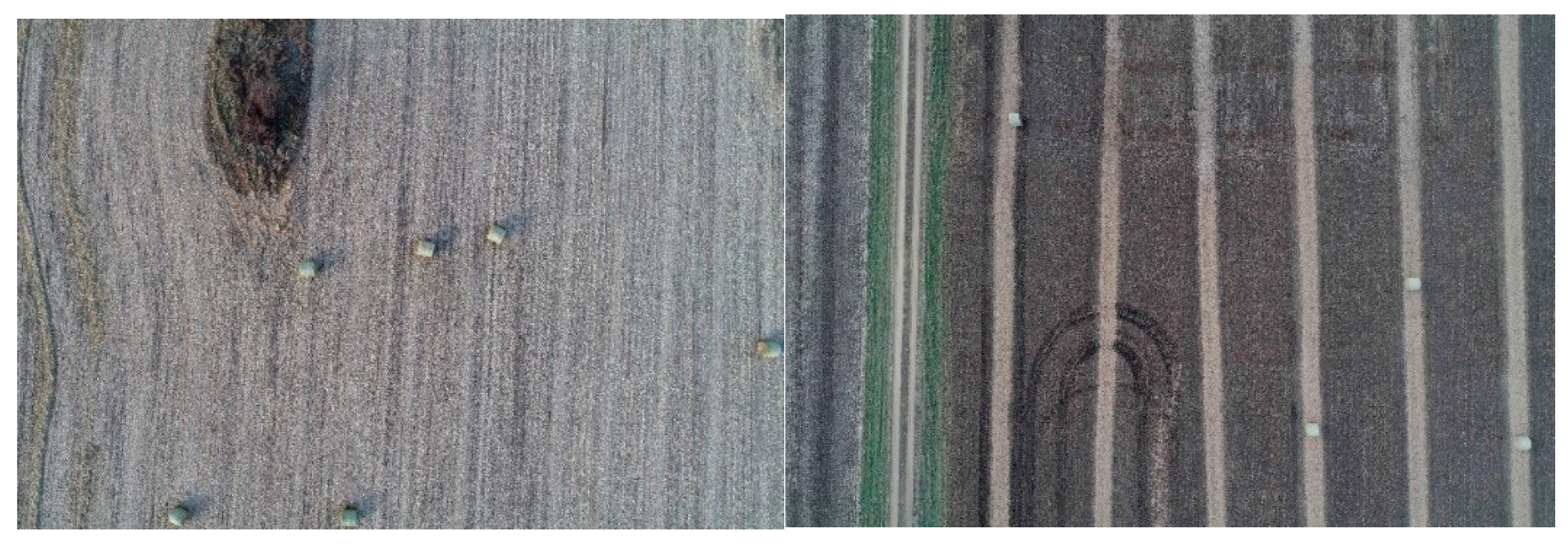
Remotesensing 13 04675 g001
Figure 2. Examples of bales imaged at 20 MP (5472 × 3648 pixels) and an altitude of 61 m above ground level yielding a pixel resolution of 1.08 × 1.65 cm: top left—field of corn stover residue containing six bales and one partial bale; top right—field of corn stover residue containing three bales and one building; bottom left—field of corn stover residue containing six bales; bottom right—field of soybean residue containing four bales.
Remotesensing 13 04675 g002aRemotesensing 13 04675 g002b
Figure 3. Examples of annotated images with LabelMe [27]: Left—a road annotated in red and four bales in blue/yellow/green/pink; right—here, a truck is highlighted in red, and yellow/green represent annotated buildings.
Remotesensing 13 04675 g003
Figure 4. Pipeline to detect bales in the field using image processing. It starts with converting the image to grayscale, blurring to remove noise, equalizing the histogram to remap the pixel values between 0–255, binarizing using Otsu threshold, and applying the erosion + dilation to remove noise.
Remotesensing 13 04675 g004
Figure 5. Sample picture from a field of corn stover residue processed through each step of the pipeline (af) described in Figure 4. The input image contains only one biomass bale in the top right part of the figure. The output image is a binary mask that segments the bale from the background.
Remotesensing 13 04675 g005
Figure 6. Image processing, faster R-CNN, and YOLOv3 detection outputs from a sample image of field 0. (a) is the original 20 MP sample image. (b) is the output of the detection using the image processing pipeline. (c,e) are the outputs of the faster R-CNN and YOLOv3 on the 1 MP sample image, respectively. (d,f) are the outputs of the faster R-CNN on the 20 MP sample image, respectively.
Remotesensing 13 04675 g006aRemotesensing 13 04675 g006b
Figure 7. The final pipeline of the mapping framework: (1) image data were collected with a UAV; (2) a YOLOv3 model was trained and tuned to obtain the coordinates in the image; (3) image coordinates are converted from drone position and pose to latitude and longitude; (4) multiple observations of the same bale in different images are reconciled using DBSCAN; (5) final coordinates of the bale is predicted.
Remotesensing 13 04675 g007
Figure 8. Field 0: (a) black dots are the predictions, and the red dots are the ground truth coordinates of the bales; (b) shows the DBSCAN clustering of the detected bales. It is possible to see that some isolated detections are rejected as noise; (c) shows an overlay of the orthomosaic with the colored DBSCAN clustering.
Remotesensing 13 04675 g008
Figure 9. The black line is the linear regression of the predicted bale location by the surveyed ground truth location of the bales. In the red dashed line, we have the 45° slope as a reference: left—predicted latitude versus actual latitude (y = 1.000629x, R2 = 1, F = 8.7 × 10⁷, p-value < 0.01); right—predicted longitude versus actual longitude (y = 1.001x, R2 = 1, F = 1.14 × 10⁸, p-value < 0.01).
Remotesensing 13 04675 g009
Table 1. Number of instances annotated using LabelImg for COCO datasets and YOLO datasets.
ImagesBalesBuildingsStreetsTrucks
300783227217
Table 2. Dataset specifications for training machine learning algorithms.
DatasetResolutionTrainValidationTest
High Res5472 × 36482432730
Low Res1080 × 7202432730
Table 3. YOLOv3 detector network architecture.
TypeFiltersSizeOutput
Convolutional323 × 3256 × 256
Convolutional643 × 3/2128 × 128
Convolutional321 × 1
1 × Convolutional643 × 3
Residual 128 × 128
Convolutional1283 × 3/264 × 64
Convolutional641 × 1
2 × Convolutional1283 × 3
Residual 64 × 64
Convolutional2563 × 3/232 × 32
Convolutional1281 × 1
8 × Convolutional2563 × 3
Residual 32 × 32
Convolutional5123 × 3/216 × 16
Convolutional2561 × 1
8 × Convolutional5123 × 3
Residual 16 × 16
Convolutional10243 × 3/28 × 8
Convolutional5121 × 1
4 × Convolutional10243 × 3
Residual 8 × 8
Avgpool Global
Connected 1000
Softmax
Table 4. Google Colab specifications of the machine used to implement the detection algorithms.
CPUMemoryGPUCUDA Version
Intel Xeon 2.20GHz16 GBTesla P100-16GB10.1
Table 5. Image processing parameters that yielded the best contrast between the bales and ground.
Gaussian SizeGaussian IterationsErosion KernelDilation KernelErosion IterationsDilation Iterations
(45.3)2(20, 20)(25, 25)12
Table 6. Performance of image processing, R-CNN, and YOLOv3 on in-field detection of biomass bales.
MethodPrecisionRecallF1mAPInference Time (s)
Image Processing0.6810.8780.767-9.1
Faster R-CNN (Low Res)0.8230.9020.8600.8020.597
Faster R-CNN (High Res)0.8450.8950.8690.8080.627
YOLOv3 (Low Res)0.7900.9670.8830.9580.377
YOLOv3 (High Res)0.8010.9880.8890.9650.400
F1—average between precision and recall; mAP— mean average precision.
Table 7. Optimal YOLOv3 hyperparameters determined for in-field detection of biomass bales.
GIoUclsclspwobjobjpw
Initial3.5437.41.049.51.0
Final5.2141.41.649.51.46
iot_tlrSGDweight_decayfl_gamma
Initial0.2250.0060.9370.00050.4
Final0.1660.0090.8810.00030.0
Table 8. Bale detection performance of YOLOv3 before and after tuning the hyperparameters.
MethodPrecisionRecallF1mAPMethod
No Tuning0.8010.9880.8890.965No Tuning
Tuned0.8951.0000.9880.945Tuned
Table 9. Bale localization performance in three fields using the proposed method compared with RTK–GNSS ground survey.
FieldRMSE (°)RMSELAT (°)RMSELON (°)RMSE (m)RMSELAT (m)RMSELON (m)
0 2.405 × 10 5 1.195 × 10 5 2.087 × 10 5 2.671.332.32
1 2.233 × 10 5 7.897 × 10 6 2.089 × 10 5 2.480.882.32
2 1.916 × 10 5 1.371 × 10 5 2.337 × 10 5 2.131.522.60
Average 2.185 × 10 5 1.119 × 10 5 2.171 × 10 5 2.431.242.41
Publisher’s Note: MDPI stays neutral with regard to jurisdictional claims in published maps and institutional affiliations.

