An Adaptive-Parameter Pixel Unmixing Method for Mapping Evergreen Forest Fractions Based on Time-Series NDVI: A Case Study of Southern China

Abstract

Spectral unmixing remains the most popular method for estimating the composition of mixed pixels. However, the spectral-based unmixing method cannot easily distinguish vegetation with similar spectral characteristics (e.g., different forest tree species). Furthermore, in large areas with significant heterogeneity, extracting a large number of pure endmember samples is challenging. Here, we implement a fractional evergreen forest cover-self-adaptive parameter (FEVC-SAP) approach to measure FEVC at the regional scale from continuous intra-year time-series normalized difference vegetation index (NDVI) values derived from moderate resolution imaging spectroradiometer (MODIS) imagery acquired over southern China, an area with a complex mixture of temperate, subtropical, and tropical climates containing evergreen and deciduous forests. Considering the cover of evergreen forest as a fraction of total forest (evergreen forest plus non-evergreen forest), the dimidiate pixel model combined with an index of evergreen forest phenological characteristics (NDVIann-min: intra-annual minimum NDVI value) was used to distinguish between evergreen and non-evergreen forests within a pixel. Due to spatial heterogeneity, the optimal model parameters differ among regions. By dividing the study area into grids, our method converts image spectral information into gray level information and uses the Otsu threshold segmentation method to simulate the appropriate parameters for each grid for adaptive acquisition of FEVC parameters. Mapping accuracy was assessed at the pixel and sub-pixel scales. At the pixel scale, a confusion matrix was constructed with higher overall accuracy (87.5%) of evergreen forest classification than existing land cover products, including GLC 30 and MOD12. At the sub-pixel scale, a strong linear correlation was found between the cover fraction predicted by our method and the reference cover fraction obtained from GF-1 images (R2 = 0.86). Compared to other methods, the FEVC-SAP had a lower estimation deviation (root mean square error = 8.6%). Moreover, the proposed method had greater estimation accuracy in densely than sparsely forested areas. Our results highlight the utility of the adaptive-parameter linear unmixing model for quantitative evaluation of the coverage of evergreen forest and other vegetation types at large scales.

1. Introduction

Forests have unique ecological value, depending on their species composition [1]. The spatial distribution pattern of tree species determines the uniqueness of their ecosystem service functions, including carbon sequestration, water and soil conservation, and biodiversity [2,3,4]. As the dominant forest species in most tropical areas and some subtropical areas, evergreen trees exhibit significant differences in seasonal evapotranspiration and carbon and nitrogen cycling compared to deciduous tree [5,6,7]. Therefore, up-to-date evergreen forest spatial distribution information at very large scales is essential for effective quantitative assessment of forest ecosystem services [8,9]. Remote sensing provides the opportunity to monitor evergreen forest information quickly and effectively at large scales [10,11]. Numerous land cover classification and object extraction techniques, such as machine learning algorithms, have been developed to process remotely sensed data [12,13,14].

The mixed pixel problem presents a great challenge to accurate land cover mapping, especially at large scales using coarse-resolution images [15,16,17]. The spectrum of a mixed pixel is a combination of the spectra of the multiple land cover classes within it. Over the past few decades, researchers have proposed a series of spectral unmixing models to obtain fractional vegetation cover (FVC) at the sub-pixel scale, including models based on linear unmixing, regression, and machine learning methods [18,19,20]. Regression models establish a relationship between vegetation indexes and fractional vegetation cover, which are usually applicable only to specific areas; such relationships vary among vegetation types and regions [21]. Linear unmixing and machine learning methods are supervised approaches that require pure endmember samples from field surveys or high spatial resolution images [22,23]. However, training signatures obtained from samples may not fully represent the diversity and variability of vegetation cover types among regions or time periods [24], since they vary according to multiple factors such as surface conditions, atmospheric conditions, withered vegetation, and soil types [25,26]. In particular, differences in the underlying surface are more significant across larger regions due to spatial heterogeneity [27], which leads to time-consuming sample selection and a lack of representation for complex surfaces by unmixing models. One potential approach to solve this problem is obtaining the parameters of the pixel unmixing model automatically. This would eliminate dependence on samples, especially for large areas.

Refined vegetation type cover fraction extraction presents another serious problem. Due to the spectral similarity between fine vegetation types (e.g., deciduous forest and evergreen forest), it is difficult for spectral unmixing methods to extract fine FVC information within mixed vegetation pixels [28]. An unmixing model using multi-temporal remote sensing images has been proposed to efficiently extract the fraction of cover occupied by a range of vegetation types [29,30]. However, the FVC models based on multi-temporal images are limited to small or specific areas due to the requirement of vast quantities of data. Most studies have focused on the use of phenological features to extract fine vegetation type cover fraction information [14,31,32,33]. However, the extraction of large-scale FVC information based on phenological characteristics is hindered by a critical problem. The acquisition of key phenological characteristics requires dense intra-year time-series data, but collection of the required images for the study period may be impeded by clouds [34,35,36]. Thus, fine temporal resolution images would enhance the accuracy of FVC extraction.

To extract evergreen forest cover fraction data for a large area, a suitable unmixing model that considers evergreen forest phenological characteristics is needed. Moderate resolution imaging spectroradiometer (MODIS) has a short revisit period (observations repeated twice per day), which enables continuous monitoring of vegetation phenological information over a large scale [37,38,39,40,41,42,43]. Although a recent study developed a linear evergreen forest cover fraction extraction model using MODIS intra-year time series data, the spatial heterogeneity and large workload issues have not been resolved at large regional scales [44].

Therefore, in this study, we developed a self-adaptive parameter (SAP) linear decomposition model to estimate fractional evergreen forest cover (FEVC) at large scales. Using the MODIS normalized difference vegetation index (NDVI) intra-year time-series dataset and Google Earth Engine (GEE), we extracted FEVC information for southern China. To reduce spatial heterogeneity, this approach divides the study area into grids and obtains optimal parameter values for the unmixing model in each grid cell. After transforming the spectral information into gray level information, the parameters are automatically optimized using an automatic threshold selection method based on gray level histograms (Otsu) and vegetation cover differences among grid cells. The Otsu method automatically obtains the optimal threshold for object and background segmentation [45]. The FEVC-SAP model does not require many endmember samples, which improves its efficiency and ensures the accuracy of sub-pixel evergreen forest mapping across a large area. The pixel unmixing model with SAPs can also be used to estimate other types of vegetation cover within a pixel, even at the national or global scale.

2. Materials and Methods

2.1. Study Area

The study area is southern China and includes 13 provinces. The total land area is 2.6 million square kilometers, which is approximately 30% of the total area of China. Most of the study area is located in the subtropical zone; only small parts are located in the tropical and warm temperate zones. The average annual precipitation throughout the study area is >800 mm, and the average winter temperature is >0 °C. Forest cover accounts for more than half of the total study area, with diverse forest tree species including evergreen needle, deciduous needle, deciduous broadleaf, and evergreen broadleaf species (Figure 1). Evergreen species are dominant throughout the study area, accounting for >80% of the total forest area (http://www.forestry.gov.cn/data.html, accessed on 7 January 2020). Significant spatial heterogeneity exists in this large region due to differences in topography, light angle, sensor angle, atmospheric conditions, and vegetation and soil types.

2.2. Data Preprocessing

MODIS NDVI data were used to derive the FEVC. We collected 16-day 250 m MODIS NDVI products for 2017 and 2018 (MOD13Q1 and MYD13Q1) from the National Aeronautics and Space Administration (NASA) Earth data website (https://search.earthdata.nasa.gov/search, accessed on 2 March 2020). Both data preprocessing and evergreen forest cover fraction estimates were carried out using the GEE platform [46]. Combining the MOD13Q1 and MYD13Q1 products, the intra-annual NDVI time-series dataset consists of 46 scene images per year for 2017 and 2018. Although MOD13Q1 and MYD13Q1 include the highest-quality pixels within the 16-day period, some pixels were affected by clouds and thus showed abnormal values; removing the effects of clouds is crucial. The maximum value composite (MVC) method was used to minimize contamination and atmospheric variability by combining 8-day MOD13Q1 and MYD13Q1 NDVI data into a single dataset with 16-day temporal resolution [47]. Cloud-free images from 2017 replaced cloud-contaminated images taken on the same date in 2018 (i.e., DOY 161 in 2017 and DOY 161 in 2018) based on the modified neighborhood similar pixel interpolator (MNSPI) method [48,49]. MNSPI removed most clouds from images taken across the study area. Temporal filtering was not performed in this study since both the MVC method and MNSPI removed 99% of cloud and other noise contamination, and temporal filtering could smooth the minimum NDVI of the time series data, which is an important signal for vegetation withering.

Some auxiliary data were also collected. GF-1 panchromatic/multi-spectral (PMS) in

Table 1. Description of Gaofen-1 images.

Number of Scenes	Acquisition Date	Coverage	Cloud Cover
8 scenes	1 January 2017~25 February 2017	E 99.3°~E 119.7°, N 21.6°~E 36.8°	<4%
13 scenes	1 December 2017~27 February 2018
11 scenes	1 December 2018~15 February 2019

and Google Earth images were used to evaluate the accuracy of evergreen forest extraction due to their high spatial resolution. The GF-1 PMS sensor observes solar radiation reflected by the Earth in four spectral channels distributed in the visible and near-infrared spectral ranges. GF-1 PMS has a spatial resolution of 2 m, achieved by fusing the multi-spectral and panchromatic bands. Google Earth images have a spatial resolution of 0.5 m. All GF-1 and Google Earth data were evenly distributed throughout the study area and were co-registered to the MODIS dataset. The high spatial resolution images are evenly distributed across the study area (total of 30 “scenes”). Geometric and atmospheric corrections of the GF-1 data were performed. Next, the Gaofen-1 panchromatic band and multi-spectral bands were fused into a 2-m resolution multi-spectral image. Global land cover (GLC) data for 2017 were employed to distinguish impervious surface from other land cover types, based on the unique characteristics of impervious surface such as extreme fragmentation (http://data.ess.tsinghua.edu.cn/, accessed on 5 March 2020). Based on GF-1 samples, the evergreen forest classification results calculated from the two products (30-m GLC 2015 and MODIS 500-m land cover product MCD 12Q1) were compared with our extraction results.

2.3. Otsu Threshold Selection Method

The Otsu method is a nonparametric, unsupervised method of automatic threshold selection for image segmentation proposed by [50]. The optimal threshold for distinguishing an object from the background based on the gray level is determined based on the discriminant criterion. The procedure is simple, as the gray level histogram consists of only two image classes (object and background).

The principle of this algorithm is as follows. Pixels of a given picture are represented in L gray levels [1,2,…, L]. The number of pixels at level i is n, the total number of pixels is N, and the probability of each gray value (${\mathrm{p}}_{\mathrm{i}}$) is given by:

$${\mathrm{p}}_{\mathrm{i}}=\mathrm{n}/\mathrm{N} \mathrm{i}=1,2,3,\dots \mathrm{L}$$

(1)

and,

$${{\displaystyle \sum }}_{\mathrm{i}=1}^{\mathrm{L}}{\mathrm{p}}_{\mathrm{i}}=1$$

(2)

Threshold T dichotomizes the pixels in the image into two classes (object and background) ${\mathrm{C}}_0$(1,2,3,…,T) and ${\mathrm{C}}_1$(T + 1,T + 2,T + 3,…,L). Then, the probability of occurrence (${\mathsf{\omega }}_0$) of class ${\mathrm{C}}_0$ is calculated as follows:

$${\mathsf{\omega }}_0={{\displaystyle \sum }}_{\mathrm{i}=1}^{\mathrm{T}}{\mathrm{p}}_{\mathrm{i}}={\mathsf{\omega }}_{\mathrm{T}}$$

(3)

The probability of occurrence (${\mathsf{\omega }}_1$) of class ${\mathrm{C}}_1$ is calculated as follows:

$${\mathsf{\omega }}_1=1-{\mathsf{\omega }}_{\mathrm{T}}$$

(4)

The total mean level (${\mathsf{\mu }}_{\mathrm{T}}$) of the entire image is calculated as follows:

$${\mathsf{\mu }}_{\mathrm{T}}={{\displaystyle \sum }}_{\mathrm{i}=1}^{\mathrm{L}}{\mathrm{ip}}_{\mathrm{i}}$$

(5)

The mean levels of class ${\mathrm{C}}_0$ and ${\mathrm{C}}_1$ are ${\mathsf{\mu }}_0$ and ${\mathsf{\mu }}_1$, respectively:

$${\mathsf{\mu }}_0={{\displaystyle \sum }}_{\mathrm{i}=1}^{\mathrm{T}}{\mathrm{ip}}_{\mathrm{i}}/{\mathsf{\omega }}_0, {\mathsf{\mu }}_1={{\displaystyle \sum }}_{\mathrm{i}=\mathrm{T}+1}^{\mathrm{L}}{\mathrm{ip}}_{\mathrm{i}}/{\mathsf{\omega }}_1$$

(6)

Therefore,

$${\mathsf{\mu }}_{\mathrm{T}}={\mathsf{\omega }}_0{\mathsf{\mu }}_0+{\mathsf{\omega }}_1{\mathsf{\mu }}_1$$

(7)

The class variances ${\mathsf{\sigma }}^2\mathrm{T}$ are determined as follows:

$${\mathsf{\sigma }}^2\mathrm{T}={\mathsf{\omega }}_0{\mathsf{\mu }}_0-{\mathsf{\mu }}_{\mathrm{T}}{}^2+{\mathsf{\omega }}_1{\mathsf{\mu }}_1-{\mathsf{\mu }}_{\mathrm{T}}{}^2={\mathsf{\omega }}_0{\mathsf{\omega }}_1{\mathsf{\mu }}_0-{\mathsf{\mu }}_1{}^2$$

(8)

The value of T ranges from 1 to L, and represents the optimal threshold of the Otsu algorithm when between-class variance is maximized. At present, the Otsu algorithm is the most popular method for automatically segmenting the object and background based on a gray level histogram.

2.4. FEVC Model Based on the Linear Unmixing Model and NDVI_ann-min Image

The dimidiate pixel model is a linear unmixing model, which assumes that the target vegetation and soil are invariant in terms of surface reflectance, and that a pixel signal comprises two components: soil and vegetation [51,52]. The equation is approximated by:

$$\mathrm{NDVI}=f_c\times {\mathrm{NDVI}}_{\mathrm{veg}}+\left(1-f_c\right)\times {\mathrm{NDVI}}_{\mathrm{soil}}$$

(9)

and,

$$f_c=\frac{\mathrm{NDVI}-{\mathrm{NDVI}}_{\mathrm{soil}}}{{\mathrm{NDVI}}_{\mathrm{veg}}-{\mathrm{NDVI}}_{\mathrm{soil}}}$$

(10)

where $f_c$ is the fractional green vegetation cover within the pixel, ${\mathrm{NDVI}}_{\mathrm{veg}}$ is the NDVI value of a pure vegetation pixel, and ${\mathrm{NDVI}}_{\mathrm{soil}}$ is the NDVI value of a pure soil pixel. In previous studies, the parameters ${\mathrm{NDVI}}_{\mathrm{veg}}$ and ${\mathrm{NDVI}}_{\mathrm{soil}}$ have typically been determined by collecting a large number of pure endmember samples (soil and vegetation) [53].

Based on the image of the minimum value of intra-year time-series NDVI (NDVI_ann-min), we assumed that only two components (evergreen forest and non-evergreen forest, if present; small bodies of water are neglected) within the pixels. Non-evergreen forest pixels were treated as pure endmembers since all vegetation the NDVI_ann-min image had entered dormancy except evergreen forest. If the NDVI of non-evergreen endmembers is regarded as an invariant parameter in the whole study area, the FEVC model can be converted as follows [44]:

$$\mathrm{FEVC}=\frac{{\mathrm{NDVI}}_{\mathrm{annmin}}-{\mathrm{NDVI}}_{\mathrm{non}-\mathrm{ef}}}{{\mathrm{NDVI}}_{\mathrm{ef}}-{\mathrm{NDVI}}_{\mathrm{non}-\mathrm{ef}}}$$

(11)

where NDVI_annmin is the NDVI_ann-min of an estimated pixel, NDVI_non-ef is the NDVI_ann-min value of a pure non-evergreen forest pixel, and NDVI_ef is the NDVI_ann-min value of a pure evergreen forest pixel. NDVI_ef and NDVI_non-ef correspond to ${\mathrm{NDVI}}_{\mathrm{veg}}$ and ${\mathrm{NDVI}}_{\mathrm{soil}}$ in Equation (10).

To eliminate crop and deciduous forest, the coefficient of variation (CV) was combined with the FEVC model. CV is the ratio of the standard deviation to the mean of the NDVI time series for each pixel.

For an entire vegetation growth cycle, a smaller CV value indicates a flatter vegetation growth status. Therefore, evergreen forest should have a smaller CV value than all other vegetation types; CV is calculated as follows:

$$\mathrm{CV}=\frac{\sqrt{\frac{1}{\mathrm{n}-1}\left[{{\displaystyle \sum }}_{\mathrm{i}=1}^{\mathrm{n}}{\left({\mathrm{NDVI}}_{\mathrm{i}}\right)}^2-{\left({{\displaystyle \sum }}_{\mathrm{i}=1}^{\mathrm{n}}{\mathrm{NDVI}}_{\mathrm{i}}\right)}^2\right]}}{\frac{1}{\mathrm{n}}{{\displaystyle \sum }}_{\mathrm{i}=1}^{\mathrm{n}}\left({\mathrm{NDVI}}_{\mathrm{i}}\right) }$$

(12)

For a pixel of the image i in the time-series dataset, where NDVI_i is the NDVI value of the pixel and n is the total number of images for the year. A CV threshold of 0.2 has been established to distinguish evergreen forest pixels from crop or deciduous forest pixels [44].

2.5. Automatic Acquisition of FEVC Model Parameters

An image with two components, soil and vegetation, could be converted to gray space [54], such that all pixels in the image are treated as vegetation pixels with varying proportions of vegetation. A gray level histogram of all pixels within the NDVI_ann-min image is shown in Figure 2a. Pure soil and pure vegetation pixels were the least numerous, whereas pixels with moderate vegetation cover accounted for the largest proportion of all pixels. This pattern corresponds to a normal distribution [55], as shown in Figure 2b. Generally, the NDVI maximum value within an image is considered to represent a fully vegetated pixel (NDVI_veg in the dimidiate pixel model) and the minimum NDVI value represents a full soil pixel (NDVI_soil) [56]. To remove interference from noise and outliers (extreme maximum or minimum NDVI values), the maximum and minimum values within a certain confidence interval (e.g., 95%) were generally used as model parameters NDVI_veg and NDVI_soil [57].

In Equation (11), NDVI_ef and NDVI_non-ef were determined under the assumption that NDVI_ann-min of the non-evergreen forest endmembers remained unchanged. However, actual land surface cover characteristics are often highly complex, especially for the purpose of FEVC model estimation. In the NDVI_ann-min image, non-evergreen forest pixels usually contain bare soil and withered vegetation. Due to the effects of withered vegetation, the NDVI values of non-evergreen forest pixels vary within a certain range (Figure 2c). Afterwards, all non-evergreen forest pixels in the image resemble a single curve. Finally, a bimodal curve that includes both object (evergreen forest pixels with varying proportions of evergreen forest) and background (soil mixed with withered vegetation) is formed (Figure 2d).

According to the FEVC model, when the parameter (NDVI_non-ef) was underestimated, some non-evergreen forest pixels with a higher NDVI_ann-min values than NDVI_non-ef would be mistakenly classified as evergreen forest. Considering this characteristic, the NDVI of the valley between the two peaks should be the optimal value to distinguish the object from the background (it is the highest NDVI_ann-min value of all background pixels). Meanwhile, the NDVI value of the valley of the bimodal curve in Figure 2d is correspond to the NDVI_soil of the single curve in Figure 2b. Therefore, our goal was converted to automatically obtain the NDVI value of the curve valley, which is the parameter NDVI_non-ef of the FEVC model.

The NDVI value of the curve valley is the optimal threshold that maximizes between-class (object and background) variance. For gray level histograms with significant double peaks, we used the Otsu method to determine the optimal threshold for distinguishing the object and background. However, due to the complex spatial distribution of land cover, double peaks that are curve-fitted based on different NDVI gray level histograms differ greatly, which causes the T values calculated using the Otsu method to deviate from the NDVI of the curve valley.

Therefore, we performed a deviation correction to ensure that the T value was as close as possible to the optimal curve valley NDVI threshold, which maximizes between-class variance. We found that forest canopy closure in the image affected the distribution of the histogram, changing the shapes of the double peaks. Generally, NDVI > 0.5 indicates a high proportion of vegetation within the pixel [58]. Therefore, pixels at NDVI_ann-min > 0.5 were identified as evergreen forest pixels and the proportion of these pixels in the image (fvc_oa) was calculated. Figure 3 shows the different gray level histograms of evergreen forest (object) pixels and non-evergreen forest (background) pixels in various NDVI_ann-min images. As the proportion of forest cover in the image increased, the T value approached the curve valley (optimal threshold).

Next, we divided the entire study area image into small pieces and extracted >90 pieces as samples. Each sample could be regarded as a small image to generate a gray level histogram. Fvc_oa, T, and the optimal threshold were calculated for each sample. Linear correlations were established among T, the optimal threshold, and fvcoa as follows:

$$\mathrm{T}-\mathrm{T}\prime =\mathrm{K}\times {\mathrm{fvc}}_{\mathrm{oa}}+\mathrm{b}$$

(13)

where T′ (is also the optimal threhold of Otsu) is the optimal threshold that maximizes between-class variance (NDVI_ann-min from the curve valley), and K and b are obtained from regression analysis of the samples, as shown in Figure 3d. The final equation is:

$$\mathrm{T}-\mathrm{T}\prime =0.3\times {\mathrm{fvc}}_{\mathrm{oa}}+0.0083$$

(14)

The FEVC model parameter (NDVI_non-ef) that takes actual surface characteristics into account is automatically obtained, and replaced with. The other parameter of the FEVC model (NDVI_ef) is estimated based on the maximum value, within a confidence interval defined according to previous studies [51]. NDVI_ef is not affected by complex soil types or withered vegetation.

2.6. Gridded Adaptive Parameters Estimation Model

Complex terrain and uneven land cover lead to spatial heterogeneity of the land surface. The parameters of the FEVC model are sensitive to spatial heterogeneity. Variations caused by terrain undulations, sun altitude differences, sensor angle differences, and physical properties generate spectral reflectance differences within a given type of land cover [59]. We analyzed seven soil and vegetation samples from various regions. Evergreen forest samples differed markedly in texture and color depth, whereas color difference between soil samples were more obvious (Figure 4). Vegetation spectral reflectance is influenced by vegetation color and growth period, while soil spectral reflectance is affected by soil type, color, and roughness, resulting in differences between NDVI_soil and NDVI_veg. Therefore, selecting only one set of parameters for the whole study area is unreasonable.

We developed an FEVC-SAP model to estimate the fraction of evergreen forest at the grid scale. The entire study area was divided into multiple smaller images of equal size by applying gridding. In each grid cell, the image was converted into binary space. The two main parameters (NDVI_non-ef and NDVI_ef) were calculated using the corrected Otsu method, and automatically optimized and adjusted according to the characteristics of the gray level histogram for each grid cell (Figure 5). The grid is similar to a sliding window. After the necessary parameters are obtained by FEVC-SAP for one grid cell, the calculations for the adjacent cell begin.

The size of the grid is pivotal to the results of the FEVC-SAP model and should be set carefully, as the degree of interference of spatial heterogeneity with the FEVC parameters is strongly related to grid size. In general, spatial heterogeneity is greater in a larger area. Therefore, a larger grid size increases the complexity of spatial heterogeneity within the grid, whereas an extremely small grid lacks many typical land use types. Therefore, we established three grid sizes (20 km × 20 km, 60 km × 60 km, and 100 km × 1000 km) and analyzed the effect of grid size on model parameter evaluation accuracy.

Next, we evaluated the accuracy of NDVI_non-ef and NDVI_ef parameter estimation in grids with different sizes according to the deviation between reference values and sample predicted values. Samples representing pure non-evergreen forest and pure evergreen forest endmembers were collected from GF-1 2 m resolution images.

2.7. Accuracy Assessment

We assessed the estimation accuracy of FEVC-SAP for evergreen forest cover using 2 m resolution GF-1 and 0.5 m resolution Google Earth images taken in winter. We selected a total of 2044 samples (0.5 km × 0.5 km) that were randomly distributed in the study area. Each sample covered four MODIS pixels; the mean of evergreen cover fraction of these four MODIS pixels was calculated to reduce the registration deviation between the MODIS and Gaofen-1 data. The resulting confusion matrix (

Table 2. Confusion matrix.

	Actual Results
		Class 1	Class 2	Class n
Predicted results	Class 1	P11	P12	P1n
	Class 2	P21	P22	P2n
	…	…	…	…
	Class n	Pn1	Pn2	Pnn

) was used to assess the accuracy of evergreen forest cover pixel extraction.

Using the confusion matrix, we calculated the producer’s accuracy (PA), user’s accuracy (UA), and overall accuracy (OA), where j is the jth class of predicted results and i is the ith class of actual results (in Table 2); classification accuracy was compared between the GLC 30 and MCD12Q1 products [60]

$$\mathrm{PA}=\frac{{\mathrm{P}}_{\mathrm{j},\mathrm{j}}}{{{\displaystyle \sum }}_{\mathrm{i}=1}^{\mathrm{n}}{\mathrm{P}}_{\mathrm{i},\mathrm{j}}}$$

(15)

$$\mathrm{UA}=\frac{{\mathrm{P}}_{\mathrm{i},\mathrm{i}}}{{{\displaystyle \sum }}_{\mathrm{j}=1}^{\mathrm{n}}{\mathrm{P}}_{\mathrm{i},\mathrm{j}}}$$

(16)

$$\mathrm{OA}=\frac{{{\displaystyle \sum }}_{\mathrm{i}=1}^{\mathrm{n}}{\mathrm{P}}_{\mathrm{i},\mathrm{i}}}{{{\displaystyle \sum }}_{\mathrm{i}=1}^{\mathrm{n}}{{\displaystyle \sum }}_{\mathrm{j}=1}^{\mathrm{n}}{\mathrm{P}}_{\mathrm{i},\mathrm{j}}}$$

(17)

We also calculated the root mean square error (RMSE) and mean relative error (MRE) to assess sub-pixel-scale accuracy [61].

$$\mathrm{RMSE}=\sqrt{\frac{1}{n}{{\displaystyle \sum }}_{i=1}^n{\left({\mathrm{P}}_{\mathrm{i}}-{\mathrm{R}}_{\mathrm{i}}\right)}^2}$$

(18)

$$\mathrm{MRE}=\frac{1}{\mathrm{n}}{{\displaystyle \sum }}_{\mathrm{i}=1}^{\mathrm{n}}\left|\frac{{\mathrm{P}}_{\mathrm{i}}-{\mathrm{R}}_{\mathrm{i}}}{{\mathrm{R}}_{\mathrm{i}}}\right|\times 100\%$$

(19)

where n is the number of samples, P_i is the value predicted by the FEVC-SAP model for sample i, and R_i is the reference value of sample i.

Forest spatial distribution presents a significant imbalance at the scale of the study area. To compare the accuracy of the FEVC-SAP model estimates for different regions within the study area, we divided the study area into densely forested regions (i.e., Yunnan, Guangxi, Guizhou, Guangdong, Zhejiang, Fujian, Jiangxi, and Hunan Provinces), with an overall forest cover fraction of >50%, sparsely forested regions (i.e., Anhui, Jiangsu, Shanghai, and Chongqing Provinces and part of Sichuan Province), with an overall forest cover fraction of <50%, and snow-covered regions (mainly in Sichuan Province).

3. Results

3.1. Determination of Grid Size

The parameter values predicted by the FEVC-SAP model for each grid cell are shown in Figure 6. Reference values were obtained for these parameters by collecting and analyzing pure evergreen and non-evergreen forest samples. In most 20 km × 20 km grid cells, the reference NDVI_non-ef values fluctuated slightly around the predicted values. Due to the effect of mixed withered vegetation, significant deviations (>0.2) were found between the reference and predicted NDVI_non-ef values in a few grid cells. Despite those discrepancies, no reference NDVI_non-ef value had a standard deviation exceeding 0.015. Compared to 20 km × 20 km grid cells, the prediction accuracy of NDVI_non-ef is lower in 60 km × 60 km and 100 km × 100 km grid cells. As grid size increases, spatial heterogeneity becomes more prominent. Consequently, the reference NDVI_non-ef values deviated widely from the 1:1 line in 60 km × 60 km grid cells, and even more widely in 100 km × 100 km cells.

NDVI _non-ef was predicted less accurately than NDVI_ef. For 20 km × 20 km grid cells, the median reference NDVI_ef values approximate the predicted ones. Similarly, for both the 60 km × 60 km and 100 km × 100 km grid cells, the deviations of NDVI_ef reference values were smaller than those of NDVI _non-ef. The main reason for the higher prediction accuracy of NDVI_ef is that pure evergreen forest pixels are less affected by spatial heterogeneity than by the complexity of the soil background (i.e., soil type, soil color, soil moisture content, and mixing of withered vegetation). In addition to interference from forest litter or straw, soil in non-evergreen forest pixels is more diverse in terms of type, color and moisture, increasing the uncertainty of NDVI _non-ef estimations.

The prediction accuracy of NDVI_ef was highest for 20 km × 20 km grid cells. Overall, the prediction accuracy of FEVC parameters is reduced when the size of grids increases due to increased spatial heterogeneity. To ensure that sufficient background and object pixels are present in the grid to generate a gray level histogram, the grid should be ≥20 km × 20 km in size, as determined experimentally.

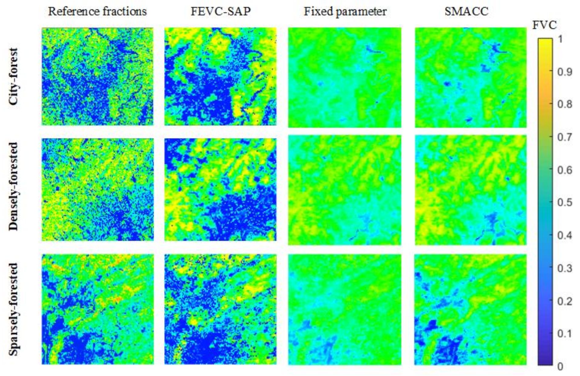
3.2. Mapping of Fractional Evergreen Forest Cover

FEVC in the study area, as determined by the FEVC-SAP model, is shown in Figure 7. Evergreen forest, especially evergreen broadleaf forest, is dominant in southern China. High evergreen forest cover fractions of 50–100% were observed throughout the study area, except for small areas in the northeast and northwest (0–30%) including Jiangsu Province, Anhui Province, Hubei Province, and high-altitude areas of northwestern Sichuan Province. Extremely low cover fractions (0–10%) were obtained for scattered evergreen trees in urban areas and cultivated fields. Moderate cover fractions (30–50%) corresponded to mixed forest in the northern provinces and regions of southern provinces where forest is adjacent to agricultural land. Notably, although the area of snow-covered evergreen forest is less than 5% of the total evergreen forest area, evergreen forest information for these areas was still considered.

Evergreen forest cover was mapped at three sites with a high degree of fidelity compared to high-resolution GF-1 images (Figure 7a). The mapping results of these three sites (designated 1–3) were enlarged, as shown in Figure 7b. The fractional cover information was generally consistent with the GF-1 images at two sites (1 and 2). At the third site, although the region was covered with snow, evergreen forest was still extracted relatively accurately.

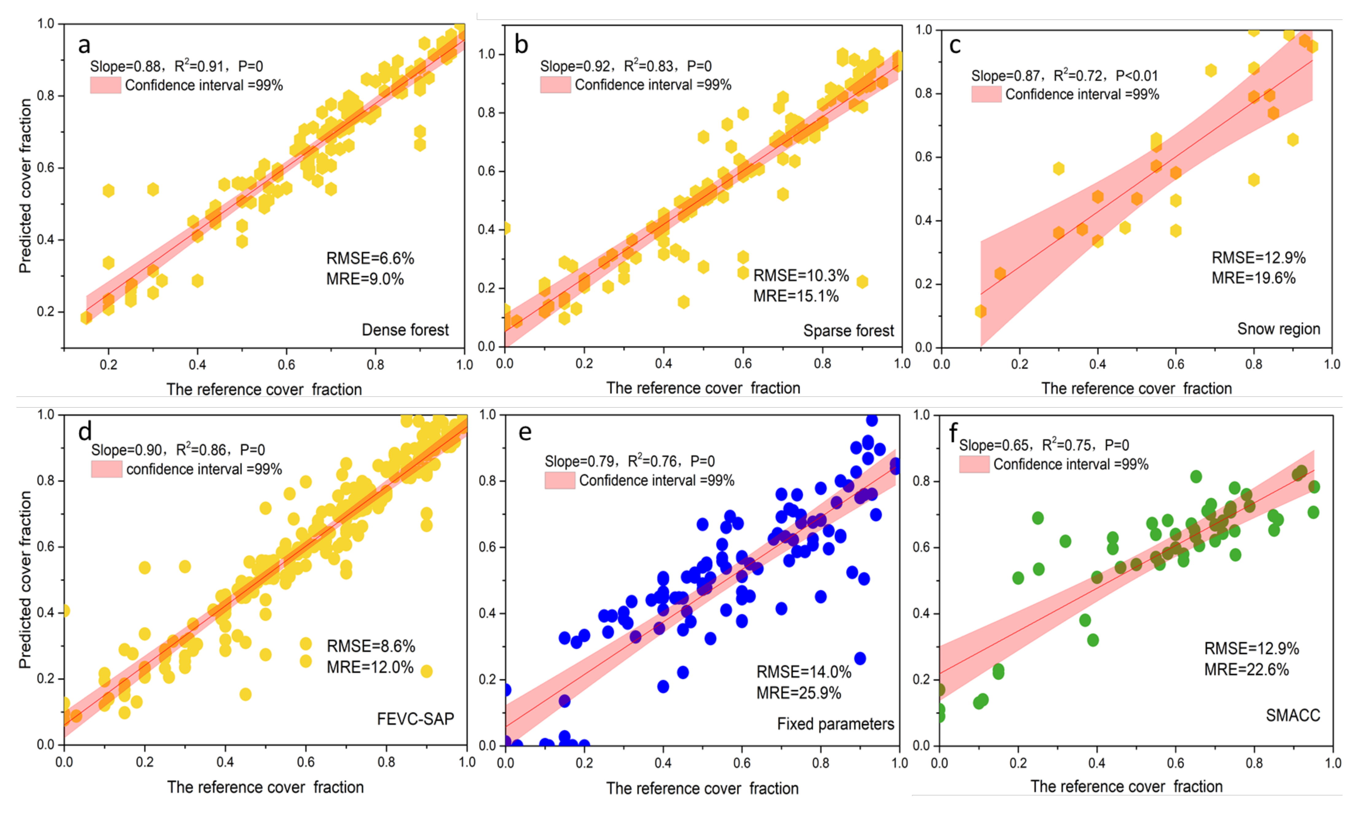
3.3. Model Accuracy Validation

The confusion matrix shown in

Table 3. Comparison of extraction accuracy of FEVC-SAP model with those of other products. UA, user accuracy; PA, producer accuracy; OA, overall accuracy.

Product	Validation Data (Number)
	Evergreen Forest		Other	UA
FEVC-SAP	Evergreen forest	828	86	90.7%
	Other	170	960	84.9%
	PA	83.3%	91.7%	OA
				87.5%
MCD 12	Evergreen forest	457	750	37.9%
	Other	161	1104	87.2%
	PA	73.9%	59.5%	OA
				63.1%
GLC 30	Evergreen forest	1016	135	88.3%
	Other	350	1055	75.1%
	PA	74.3%	88.6%	OA
				81.0%

, based on the FEVC-SAP method and MODIS dataset, revealed higher classification accuracy at the pixel scale, including PA, UA, and OA, compared with the MCD 12 land cover product; these accuracy results exceeded those of the 30 m resolution GLC 30 data. The OA of evergreen forest extraction using FEVC-SAP was 87.5%, the PA was 83.3%, and the UA was >90%. The OAs of MCD 12 and GLC 30 were 63.1% and 81.0%, respectively.

The classification accuracy for each of the three regions with different forest cover characteristics are shown in

Table 4. Comparison of extraction accuracy values among three regions based on FEVC-SAP model.

FEVC-SAP	Validation Data (Number)
Regions	Evergreen Forest		Other	UA
Dense forest	Evergreen forest	456	48	90.4%
	Other	40	204	83.6%
	PA	91.9%	80.9%	OA
				88.2%
Sparse forest	Evergreen forest	214	30	87.7%
	Other	48	358	88.1%
	PA	81.6%	92.2	OA
				88.0%
Snow region	Evergreen forest	178	18	90.8%
	Other	82	398	82.9%
	PA	68.4%	95.6%	OA
				85.2%

. In densely forested regions, the FEVC-SAP model achieved the highest OA (88.2%) and producer accuracy of 91.9% and UA of 90.4%. The OA for sparsely forested areas was slightly lower (88%), and the lowest accuracy was obtained for snow-covered regions. In sparsely forested regions, the double peak distribution shown by the gray level histogram was unclear due to an insufficient number of object (forest) pixels, which reduced prediction accuracy. Additionally, thick snow obscures evergreen forest.

Differences between the reference and predicted cover fractions (obtained using the FEVC-SAP method) at the sub-pixel scale showed similar trends to the classification accuracy (Figure 8). The prediction accuracy of FEVC-SAP was highest for the densely forest area, with a RMSE of 6.6% and MRE of 9.0%. The slope value was 0.88 and R² exceeded 0.9. When both the slope and R² are equal to 1, prediction accuracy is 100%. Both the sparsely forested and snow-covered regions had poor prediction results, with RMSE and MRE values above 10%. The R² and slope in those two regions were also lower than in the densely forest area.

For the entire study area, we also evaluated the estimation accuracy of evergreen forest cover using two other methods: the fixed-parameter method (only one set of FEVC parameters used for the entire area) and the sequential maximum angle convex cone (SMACC) method [62]. We obtained the cover fraction of multiple endmembers based on SMACC values derived from the time-series NDVI dataset. Comparing the FEVC-SAP with the other two methods (Figure 8), we found that FEVC-SAP achieved the best prediction results for FEVC, with the lowest MRE (12%) and RMSE (8.6%) values. In contrast, the evergreen forest cover prediction accuracy was relatively poor using the fixed-parameter method and SMACC, reflected in low R² and slope values, and high RMSE and MRE values.

Evergreen forest fraction results obtained from the FEVC-SAP model and two other methods for regions dominated by three types of land cover are shown in Figure 9. Compared to the reference fractions of evergreen forest cover, both the fixed-parameter method and SMACC tended to overestimate and underestimate low and high fractions of evergreen forest, respectively, in different regions. The FEVC-SAP model achieved the highest accuracy in densely-forested areas. In both sparsely forested areas and those containing adjacent forest and city, the FEVC-SAP model underestimated the fraction of evergreen forest cover when the total forest cover fraction was <0.5, and overestimated it when the total forest cover fraction was >0.8.

4. Discussion

4.1. Elimination of Large-Scale Spatial Heterogeneity Based on Grids

The dimidiate pixel model, a type of LSMM (linear spectral mixing model), is widely used to estimate fractional vegetation cover due to its sound physical basis and simple implementation. However, this model is easily affected by the complexity of surface components. For example, LSMM assumes that pure endmembers exist, and that only two components (vegetation and soil) are present in the study area [63]. These assumptions are generally applicable to an ideal case where spectral reflectance variation within each land cover class is sufficiently small. However, high spatial heterogeneity exists across large areas, leading to spectral reflectance differences within land cover classes. For extraction of the evergreen forest cover fraction, although we assumed that the two endmember components (vegetation and soil) could be replaced with evergreen and non-evergreen forest in the NDVI_ann-min image, both the evergreen and non-evergreen forest pixels were impacted by spatial heterogeneity across the large study area (Figure 4).

Taking full account of spatial heterogeneity, the FEVC-SAP model achieved relatively high estimation accuracy for fractional evergreen forest across a large area (Figure 8). We divided the study area into grid cells and ignored spatial heterogeneity within individual cells due to their small areas. Therefore, the FEVC-SAP model parameters for a single grid cell were minimally affected by spatial heterogeneity. Previous models have been unable to solve spatial heterogeneity. As shown in Figure 9, the fixed-parameter method, which is based on one set of model parameters, and the non-parametric SMACC method, simulating factors such as spatial heterogeneity in the context of an extremely complex land surface, is difficult due to a lack of training samples from evergreen and non-evergreen forest areas [64].

By applying the corrected Otsu method to the parameter selection process for the FEVC model, SAPs were automatically obtained for each grid cell. In previous vegetation cover studies that applied the dimidiate pixel model, NDVI_soil and NDVI_veg have generally been determined empirically, or based on pure soil and pure vegetation samples obtained from field sampling and high-resolution images [56]. At the national or global scale, sample collection is time-consuming, labor-intensive, and subjective [65]. In contrast, the FEVC-SAP method is less dependent on samples. This method allows rapid extraction of the evergreen forest cover fraction with high accuracy. Therefore, it is more suitable for large regions (i.e., for national and global scale studies). Moreover, FEVC-SAP makes full use of time-series data. In contrast to existing pixel decomposition methods based on spectral unmixing, the FEVC-SAP can distinguish vegetation types with high spectral similarity, such as evergreen and deciduous forests.

4.2. Applicability and Sensitivity of the FEVC-SAP Method

Due to the small number and uneven distribution of pure evergreen forest pixels in the grid, the NDVI_ef value determined from the 95% confidence intervals of the gray level histogram was lower than the true value, leading to overestimation of pixels with cover fractions near 100%. Due to the high proportion of soil (including withered vegetation), the NDVI_non-ef derived using the corrected Otsu method was higher than the actual value, resulting in underestimation of pixels with low fractions of evergreen forest. Therefore, the FEVC-SAP is most applicable in densely forested areas.

The FEVC-SAP method is also suitable for the extraction of other types of vegetation cover. The NDVI is a good indicator of vegetation growth and is also the most popular [66]. Most remote sensing images contain red and near-infrared bands, and this model can use a variety of image types. In addition, in contrast to other supervised spectral unmixing models, the Otsu method converts spectral information into gray level information, and thus does not rely on vegetation spectral features for unmixing. Once the land cover types of the study area are divided into object and background, the proposed method can be applied. Importantly, as there is no need for a large quantity of high-resolution field samples, this approach is practical at the national or global scale, but is not necessary for small areas.

4.3. Uncertainty and Future Research

In this study, we assessed the potential for evergreen forest mapping across a large and complex area using intra-year time-series NDVI data. However, there are limitations to the application of the proposed method. Although previous studies have reported advances in the use of LSMM for detailed mapping of dominant vegetation classes at the sub-pixel scale, linear decomposition may be inadequate in areas with a complex underlying surface [67]. In the proposed model, NDVI_non-ef was simulated through linear correlation using the Otsu threshold and proportion of forest in the grid. Then, NDVI_ef was predicted based on gray level confidence intervals. Complex land surfaces are difficult to simulate based on simple correlation analyses. Therefore, our method cannot guarantee high accuracy for all sites.

Time-series analysis of vegetation indexes has demonstrated utility for distinguishing among land cover types based on phenological characteristics [68]. Time-series and spectral data can be combined to accurately distinguish among vegetation types and obtain cover fractions at the sub-pixel scale in future pixel unmixing research [69]. In this paper, an attempt was made to extract information about the evergreen forest cover fraction using time-series data, and to obtain model parameters using an adaptive method. Future research should focus on improving parameter prediction accuracy. Unmixing methods that combine spectral and time-spectral data should also be further studied.

5. Conclusions

In this study, we proposed an FEVC-SAP model for estimating the fraction of evergreen forest cover. Using intra-year time-series NDVI data from MODIS, this method improved the dimidiate pixel model through adaptive parameter selection. Without relying on high-resolution images, extraction of the evergreen forest cover fraction was achieved across a large area. Despite the complexity of the land cover in the study area, the overall unmixing accuracy for evergreen forest fractions exceeded 85%. In previous studies, the FEVC model, which applies the dimidiate pixel model to time-series characteristics of evergreen forest, was effective at regional and single-city scales. Considering the influence of spatial heterogeneity on the parameters of the dimidiate pixel model, we divided the study area into grid cells and used the Otsu method to adaptively simulate the parameters in each cell. In contrast to existing studies of pixel decomposition, which obtain parameters through training with numerous samples, the FEVC-SAP method optimizes the parameters automatically according to evergreen forest distribution within the grid. Our FEVC-SAP model will allow for rapid and accurate mapping of evergreen forest cover at the sub-pixel scale. Our method has notable advantages, especially for dealing with the significant spatial heterogeneity present at national or global scales. In particular, the method presented in this study can be used to obtain high-quality information about vegetation composition in other areas around the world. Such information will be especially important in regions where field sampling is difficult or high-resolution images are scarce.

References

1. Bonan, G.B. Forests and Climate Change: Forcings, Feedbacks, and the Climate Benefits of Forests. Science 2008, 320, 1444–1449. [Google Scholar] [CrossRef] [PubMed] [Green Version]
2. Foley, J.A.; DeFries, R.; Asner, G.P.; Barford, C.; Bonan, G.; Carpenter, S.R.; Chapin, F.S.; Coe, M.; Daily, G.C.; Gibbs, H.K.; et al. Global consequences of land use. Science 2005, 309, 570–574. [Google Scholar] [CrossRef] [Green Version]
3. Pongratz, J.; Reick, C.H.; Raddatz, T.; Claussen, M. Biogeophysical versus biogeochemical climate response to historical anthropogenic land cover change. Geophys. Res. Lett. 2010, 37. [Google Scholar] [CrossRef] [Green Version]
4. Wu, X.; Wang, X.; Xia, X.; Fang, J.; Wu, Y. Forest biomass is strongly shaped by forest height across boreal to tropical forests n China. J. Plant Ecol. 2015, 8, 559–567. [Google Scholar] [CrossRef] [Green Version]
5. Morin, X.; Fahse, L.; Scherer-Lorenzen, M.; Bugmann, H. Tree species richness promotes productivity in temperate forests through strong complementarity between species. Ecol. Lett. 2011, 14, 1211–1219. [Google Scholar] [CrossRef] [PubMed]
6. Paquette, A.; Messier, C. The effect of biodiversity on tree productivity: From temperate to boreal forests. Glob. Ecol. Biogeogr. 2011, 20, 170–180. [Google Scholar] [CrossRef] [Green Version]
7. Feng, X.; Fu, B.; Piao, S.; Wang, S.; Ciais, P.; Zeng, Z.; Lü, X.F.B.F.S.W.Y.; Zeng, Y.; Li, Y.; Jiang, X.; et al. Revegetation in China’s Loess Plateau is approaching sustainable water resource limits. Nat. Clim. Chang. 2016, 6, 1019–1022. [Google Scholar] [CrossRef]
8. Baccini, A.; Goetz, S.; Walker, W.S.; Laporte, N.T.; Sun, M.; Sulla-Menashe, D.; Hackler, J.L.; Beck, P.S.A.; Dubayah, R.O.; Friedl, M.A.; et al. Estimated carbon dioxide emissions from tropical deforestation improved by carbon-density maps. Nat. Clim. Chang. 2012, 2, 182–185. [Google Scholar] [CrossRef]
9. Ørka, H.O.; Dalponte, M.; Gobakken, T.; Næsset, E.; Ene, L.T. Characterizing forest species composition using multiple remote sensing data sources and inventory approaches. Scand. J. For. Res. 2013, 28, 677–688. [Google Scholar] [CrossRef]
10. Kennedy, R.E.; Yang, Z.G.; Cohen, W.B. Detecting trends in forest disturbance and recovery using yearly Landsat time series: LandTrendr—Temporal segmentation algorithms. Remote Sens. Environ. 2010, 114, 2897–2910. [Google Scholar] [CrossRef]
11. Herold, M.; Románcuesta, R.M.; Hirata, Y.; Laake, P.V.; Asner, G.; Heymell, V. A review of methods to measure and monitor historical forest degradation. Unasylva 2012, 62, 16–24. [Google Scholar]
12. Huang, B.; Zhao, B.; Song, Y. Urban land-use mapping using a deep convolutional neural network with high spatial reso-lution multispectral remote sensing imagery. Remote. Sens. Environ. 2018, 214, 73–86. [Google Scholar] [CrossRef]
13. Kataria, A.; Singh, M. A review of data classification using k-nearest neighbour algorithm. Int. J. Emerg. Technol. Adv. Eng. 2013, 3, 354–360. [Google Scholar]
14. Miettinen, J.; Shi, C.; Tan, W.J.; Liew, S.C. 2010 land cover map of insular Southeast Asia in 250-m spatial resolution. Remote. Sens. Lett. 2012, 3, 11–20. [Google Scholar] [CrossRef]
15. Roberts, D.A.; Gardner, M.; Church, R.; Ustin, S.; Scheer, G.; Green, R.O. Mapping Chaparral in the Santa Monica Mountains Using Multiple Endmember Spectral Mixture Models. Remote. Sens. Environ. 1998, 65, 267–279. [Google Scholar] [CrossRef]
16. Jia, K.; Yang, L.; Liang, S.; Xiao, Z.; Zhao, X. Long-Term Global Land Surface Satellite (GLASS) Fractional Vegetation Cover Product Derived From MODIS and AVHRR Data. IEEE J. Sel. Top. Appl. Earth Obs. Remote. Sens. 2018, 12, 508–518. [Google Scholar] [CrossRef]
17. Plaza, A.; Martínez, P.; Pérez, R. Spatial/Spectral Endmember Extraction by Multidimensional Morpho-logical Operations. IEEE Trans. Geosci. Remote. Sens. 2002, 40, 2025–2041. [Google Scholar] [CrossRef] [Green Version]
18. Heinz, D.C.; Chang, C.I. Fully Constrained Least Squares Linear Spectral Mixture Analysis Method for Material Quantifica-tion in Hyperspectral Imagery. IEEE Trans. Geosci. Remote. Sens. 2001, 39, 529–545. [Google Scholar] [CrossRef] [Green Version]
19. Keshava, N.; Mustard, J.F. Spectral unmixing. IEEE Signal Process. Mag. 2002, 19, 44–57. [Google Scholar] [CrossRef]
20. Jia, K.; Liang, S.; Gu, X.; Baret, F.; Wei, X.; Wang, X.; Yao, Y.; Yang, L.; Li, Y. Fractional vegetation cover estimation algorithm for Chinese GF-1 wide field view data. Remote. Sens. Environ. 2016, 177, 184–191. [Google Scholar] [CrossRef]
21. Bioucas-Dias, J.M.; Plaza, A.; Dobigeon, N.; Parente, M.; Du, Q.; Gader, P.; Chanussot, J. Hyperspectral Unmixing Overview: Geometrical, Statistical, and Sparse Regression-Based Approaches. IEEE J. Sel. Top. Appl. Earth Obs. Remote Sens. 2012, 5, 354–379. [Google Scholar] [CrossRef] [Green Version]
22. Heylen, R.; Parente, M.; Gader, P. A Review of Nonlinear Hyperspectral Unmixing Methods. IEEE J. Sel. Top. Appl. Earth Obs. Remote Sens. 2014, 7, 1844–1868. [Google Scholar] [CrossRef]
23. Qu, Y.; Wang, J.; Wan, H.; Li, X.; Zhou, G. A Bayesian network algorithm for retrieving the characterization of land surface vegetation. Remote. Sens. Environ. 2008, 112, 613–622. [Google Scholar] [CrossRef]
24. Xiao, J.; Moody, A. A comparison of methods for estimating fractional green vegetation cover within a desert-to-upland transition zone in central New Mexico, USA. Remote. Sens. Environ. 2005, 98, 237–250. [Google Scholar] [CrossRef]
25. Price, J.C. On the information content of soil reflectance spectra. Remote. Sens. Environ. 1990, 33, 113–121. [Google Scholar] [CrossRef]
26. Jacquemoud, S.; Verhoef, W.; Baret, F.; Bacour, C.; Zarco-Tejada, P.J.; Asner, G.P.; François, C.; Ustin, S.L. PROSPECT+SAIL models: A review of use for vegetation characterization. Remote. Sens. Environ. 2009, 113, S56–S66. [Google Scholar] [CrossRef]
27. Johnson, B.; Tateishi, R.; Kobayashi, T. Remote Sensing of Fractional Green Vegetation Cover Using Spatially-Interpolated Endmembers. Remote. Sens. 2012, 4, 2619–2634. [Google Scholar] [CrossRef] [Green Version]
28. Yuan, H.; Wu, C.; Lu, L.; Wang, X. A new algorithm predicting the end of growth at five evergreen conifer forests based on nighttime temperature and the enhanced vegetation index. ISPRS J. Photogramm. Remote. Sens. 2018, 144, 390–399. [Google Scholar] [CrossRef]
29. Bullock, E.L.; Woodcock, C.E.; Olofsson, P. Monitoring tropical forest degradation using spectral unmixing and Landsat time series analysis. Remote. Sens. Environ. 2020, 238, 110968. [Google Scholar] [CrossRef]
30. Wang, Q.; Ding, X.; Tong, X.; Atkinson, P.M. Spatio-temporal spectral unmixing of time-series images. Remote. Sens. Environ. 2021, 259, 112407. [Google Scholar] [CrossRef]
31. Achard, F.; Eva, H.; Mayaux, P. Tropical forest mapping from coarse spatial resolution satellite data: Production and accuracy assessment issues. Int. J. Remote. Sens. 2001, 22, 2741–2762. [Google Scholar] [CrossRef]
32. Kou, W.; Liang, C.; Wei, L.; Hernandez, A.J.; Yang, X. Phenology-Based Method for Mapping Tropical Evergreen Forests by Integrating of MODIS and Landsat Imagery. Forests 2017, 8, 34. [Google Scholar] [CrossRef]
33. Qin, Y.; Xiao, X.; Dong, J.; Zhang, G.; Roy, P.S.; Joshi, P.K.; Gilani, H.; Murthy, M.S.R.; Jin, C.; Wang, J.; et al. Mapping forests in monsoon Asia with ALOS PALSAR 50-m mosaic images and MODIS imagery in 2010. Sci. Rep. 2016, 6, 20880. [Google Scholar] [CrossRef] [PubMed]
34. Healey, S.P.; Cohen, W.B.; Spies, T.A.; Moeur, M.; Pflugmacher, D.; Whitley, M.G.; Lefsky, M. The Relative Impact of Harvest and Fire upon Landscape-Level Dynamics of Older Forests: Lessons from the Northwest Forest Plan. Ecosystems 2008, 11, 1106–1119. [Google Scholar] [CrossRef] [Green Version]
35. Lo, C.P.; Choi, J. A hybrid approach to urban land use/cover mapping using Landsat 7 Enhanced Thematic Mapper Plus (ETM+) images. Int. J. Remote. Sens. 2004, 25, 2687–2700. [Google Scholar] [CrossRef]
36. Masek, J.G.; Huang, C.; Wolfe, R.; Cohen, W.; Hall, F.; Kutler, J.; Nelson, P. North American forest disturbance mapped from a decadal Landsat record. Remote. Sens. Environ. 2008, 112, 2914–2926. [Google Scholar] [CrossRef]
37. Funk, C.; Budde, M.E. Phenologically-tuned MODIS NDVI-based production anomaly estimates for Zimbabwe. Remote Sens. Environ. 2009, 113, 115–125. [Google Scholar] [CrossRef]
38. Mildrexler, D.J.; Zhao, M.; Running, S.W. Testing a MODIS Global Disturbance Index across North America. Remote. Sens. Environ. 2009, 113, 2103–2117. [Google Scholar] [CrossRef]
39. Roy, D.P.; Jin, Y.; Lewis, P.E.; Justice, C.O. Prototyping a global algorithm for systematic fire-affected area mapping using MODIS time series data. Remote. Sens. Environ. 2005, 97, 137–162. [Google Scholar] [CrossRef]
40. Spruce, J.P.; Sader, S.; Ryan, R.E.; Smoot, J.; Kuper, P.; Ross, K.; Prados, D.; Russell, J.; Gasser, G.; McKellip, R. Assessment of MODIS NDVI time series data products for detecting forest defoliation by gypsy moth outbreaks. Remote. Sens. Environ. 2011, 115, 427–437. [Google Scholar] [CrossRef]
41. Verbesselt, J.; Hyndman, R.; Newnham, G.; Culvenor, D. Detecting trend and seasonal changes in satellite image time series. Remote Sens. Environ. 2010, 114, 106–115. [Google Scholar] [CrossRef]
42. Wardlow, B.D.; Egbert, S.L.; Kastens, J.H. Analysis of time-series MODIS 250 m vegetation index data for crop classification in the U.S. Central Great Plains. Remote. Sens. Environ. 2007, 108, 290–310. [Google Scholar] [CrossRef] [Green Version]
43. Zhan, X.; Sohlberg, R.A.; Townshend, J.R.G.; DiMiceli, C.; Carroll, M.L.; Eastman, J.C.; Hansen, M.C.; DeFries, R.S. Detection of land cover changes using MODIS 250 m data. Remote. Sens. Environ. 2002, 83, 336–350. [Google Scholar] [CrossRef]
44. Yang, Y.; Wu, T.; Wang, S.; Li, H. Fractional evergreen forest cover mapping by MODIS time-series FEVC-CV methods at sub-pixel scales. ISPRS J. Photogramm. Remote. Sens. 2020, 163, 272–283. [Google Scholar] [CrossRef]
45. Xiao, L.; Ouyang, H.; Fan, C. An improved Otsu method for threshold segmentation based on set mapping and trapezoid region intercept histogram. Optik 2019, 196, 163106. [Google Scholar] [CrossRef]
46. Gorelick, N.; Hancher, M.; Dixon, M.; Ilyushchenko, S.; Thau, D.; Moore, R. Google Earth Engine: Planetary-scale geospatial analysis for everyone. Remote Sens. Environ. 2017, 202, 18–27. [Google Scholar] [CrossRef]
47. Marcal, A.R.S.; Wright, G.G. The use of ’overlapping’ NOAA-AVHRR NDVI maximum value composites for Scotland and initial comparisons with the land cover census on a Scottish Regional and District basis. Int. J. Remote. Sens. 1997, 18, 491–503. [Google Scholar] [CrossRef] [Green Version]
48. Shen, H.; Li, H.; Qian, Y.; Zhang, L.; Yuan, Q. An effective thin cloud removal procedure for visible remote sensing images. ISPRS J. Photogramm. Remote. Sens. 2014, 96, 224–235. [Google Scholar] [CrossRef]
49. Zhu, Z.; Woodcock, C.E. Object-based cloud and cloud shadow detection in Landsat imagery. Remote. Sens. Environ. 2012, 118, 83–94. [Google Scholar] [CrossRef]
50. Ostu, N.; Nobuyuki, O.; Otsu, N. A thresholding selection method from gray level histogram. IEEE SMC-8 1979, 9, 62–66. [Google Scholar] [CrossRef] [Green Version]
51. Wu, B.F.; Li, M.M.; Yan, C.Z.; Zhou, W.F.; Yan, C.Z. Developing Method of Vegetation FRACTION estimation by Remote Sensing for Soil Loss Equation: A Case in the Upper Basin of Miyun Reservoir. In Proceedings of the 2004 IEEE International Geoscience and Remote Sensing Symposium, Anchorage, AK, USA, 20–24 September 2004; pp. 4352–4355. [Google Scholar]
52. Ding, Y.; Zhang, H.; Li, Z.; Xin, X.; Zheng, X.; Zhao, K. Comparison of fractional vegetation cover estimations using dimidiate pixel models and look-up table inversions of the PROSAIL model from Landsat 8 OLI data. J. Appl. Remote. Sens. 2016, 10, 36022. [Google Scholar] [CrossRef]
53. Qi, J.; Marsett, R.C.; Moran, M.S.; Goodrich, D.C.; Heilman, P.; Kerr, Y.; Dedieu, G.; Chehbouni, A.; Zhang, X. Spatial and temporal dynamics of vegetation in the San Pedro River basin area. Agric. For. Meteorol. 2000, 105, 55–68. [Google Scholar] [CrossRef] [Green Version]
54. Gonzalez, R.C.; Woods, R.E. Digital Image Processing; Prentice Hall International: Hoboken, NJ, USA, 2008; Volume 28, pp. 484–486. [Google Scholar]
55. Teng, S.P.; Chen, Y.K.; Cheng, K.S.; Lo, H.C. Hypothesis-test-based land cover change detection using multi-temporal satellite images—A comparative study. Adv. Space Res. 2008, 41, 1744–1754. [Google Scholar] [CrossRef]
56. Qi, J.; Kerr, Y.; Chehbouni, A. External factor consideration in vegetation index development. Val D’isere 1994, 1, 17–21. [Google Scholar]
57. Zhang, X.; Wu, B. A temporal transformation method of fractional vegetation cover derived from high and moderate resolution remote sensing data. Acta Ecol. Sin. 2015, 35, 1155–1164. [Google Scholar] [CrossRef] [Green Version]
58. Carlson, T.N.; Ripley, D.A. On the relation between NDVI, fractional vegetation cover, and leaf area index. Remote. Sens. Environ. 1997, 62, 241–252. [Google Scholar] [CrossRef]
59. Kaufman, Y.J.; Tanre, D. Atmospherically resistant vegetation index (ARVI) for EOS-MODIS. IEEE Trans. Geosci. Remote Sens. 1992, 30, 261–270. [Google Scholar] [CrossRef]
60. Xu, J.; Zhang, Y.; Miao, D. Three-way confusion matrix for classification: A measure driven view. Inf. Sci. 2020, 507, 772–794. [Google Scholar] [CrossRef]
61. Mentaschi, L.; Besio, G.; Cassola, F.; Mazzino, A. Problems in RMSE-based wave model validations. Ocean Model. 2013, 72, 53–58. [Google Scholar] [CrossRef]
62. Gruninger, J.H.; Ratkowski, A.J.; Hoke, M.L. The sequential maximum angle convex cone (SMACC) endmember model. Algorithms Technol. Multispectral Hyperspectral Ultraspectral Imag. X 2004, 5425, 1–14. [Google Scholar] [CrossRef]
63. Zeng, X.; Dickinson, R.E.; Walker, A.; Shaikh, M.; DeFries, R.S.; Qi, J. Derivation and Evaluation of Global 1-km Fractional Vegetation Cover Data for Land Modeling. J. Appl. Meteorol. 2000, 39, 826–839. [Google Scholar] [CrossRef]
64. Zhang, C.; Ma, L.; Chen, J.; Rao, Y.; Zhou, Y.; Chen, X. Assessing the impact of endmember variability on linear Spectral Mixture Analysis (LSMA): A theoretical and simulation analysis. Remote. Sens. Environ. 2019, 235, 111471. [Google Scholar] [CrossRef]
65. Metzler, J.W.; Sader, S.A. Model development and comparison to predict softwood and hardwood per cent cover using high and medium spatial resolution imagery. Int. J. Remote. Sens. 2005, 26, 3749–3761. [Google Scholar] [CrossRef]
66. Hassan, M.A.; Yang, M.; Rasheed, A.; Yang, G.; Reynolds, M.P.; Xia, X.; Xiao, Y.; He, Z. A rapid monitoring of NDVI across the wheat growth cycle for grain yield prediction using a multi-spectral UAV platform. Plant Sci. 2019, 282, 95–103. [Google Scholar] [CrossRef]
67. Jiménez-Muñoz, J.C.; Sobrino, J.A.; Plaza, A.; Guanter, L.; Moreno, J.; Martinez, P. Comparison Between Fractional Vegetation Cover Retrievals from Vegetation Indices and Spectral Mixture Analysis: Case Study of PROBA/CHRIS Data Over an Agricultural Area. Sensors 2009, 9, 768–793. [Google Scholar] [CrossRef]
68. Dymond, C.C.; Mladenoff, D.J.; Radeloff, V.C. Phenological differences in Tasseled Cap indices improve deciduous forest classification. Remote. Sens. Environ. 2002, 80, 460–472. [Google Scholar] [CrossRef]
69. Zurita-Milla, R.; Gómez-Chova, L.; Guanter, L.; Clevers, J.G.P.W.; Camps-Valls, G. Multitemporal Unmixing of Medium-Spatial-Resolution Satellite Images: A Case Study Using MERIS Images for Land-Cover Mapping. IEEE Trans. Geosci. Remote Sens. 2011, 49, 4308–4317. [Google Scholar] [CrossRef]
Figure 1. Forest distribution in southern China in 2010.
Remotesensing 13 04678 g001
Figure 2. Gray level histograms of NDVI in single-value and binary space. (b) Curve fitting the NDVI frequency histogram shown in (a). The parameters and R2 of the fitted Gaussian function are listed in Table in (b,d). (d) Bimodal curve fitting of the NDVI frequency histogram in shown in (c). Peak 1 is the Gaussian curve of the background (non-evergreen forest); Peak 2 is the Gaussian curve for object (evergreen forest).
Remotesensing 13 04678 g002
Figure 3. The influence of forest coverage on the shape of gray level histogram. (ac) Gray level histograms of the “overall forest coverage”; (d) linear fit between overall forest coverage (fvcoa) and (T–T’).
Remotesensing 13 04678 g003
Figure 4. Spatial heterogeneity among vegetation and soil. (A) a~f: color contrasts indicate differences among vegetation and soil cover in different regions; (B) data from the United States Geological Survey (USGS) Advanced Spaceborne Thermal Emission and Reflection Radiometer (ASTER) spectral library. a and b, reflectance differences between forest with different leaf colors and growth period; c, reflectance difference among three soils.
Remotesensing 13 04678 g004
Figure 5. Schematic of the evergreen forest extraction process using the FEVC-SAP model. (P1′ and P2′ represent the optimal parameters in the grid respectively; and P1′′ and P2′′ represent the optimal parameters in another grid, respectively).
Remotesensing 13 04678 g005
Figure 6. Parameter simulation accuracy by grid size. Red line represents the error between reference value and prediction value of NDVInon-ef, Green line represents the error between reference value and prediction value of NDVIef.
Remotesensing 13 04678 g006
Figure 7. Evergreen forest cover in the study area. 1(a), 2(a), and 3(a) are false-color composite images produced by combining GF-1 blue, green, and red bands obtained in winter (31 December 2017; 16 January 2018; and 2 February 2018) for areas corresponding to red boxes 1–3 on the map. 1(b), 2(b), and 3(b) are magnifications of 1(a), 2(a), and 3(a), respectively.
Remotesensing 13 04678 g007
Figure 8. Predicted and reference evergreen forest cover values for regions dominated by three types of land cover, obtained using the fixed-parameter method and SMACC methods. (ac are accuracy comparisons in different regions and df are accuracy comparisons of different models).
Remotesensing 13 04678 g008
Figure 9. Evergreen forest fractions for three different sites (urban forest, urban area, and a region containing their border) generated using the FEVC-SAP model, the fixed-parameter method, and SMACC. The reference fractions were derived from GF-1 images taken in winter. Fractions range from 0 (blue) to 1 (yellow).
Remotesensing 13 04678 g009