Abstract
High-resolution Synthetic Aperture Radar (SAR), as an efficient Earth observation technology, can be used as a complementary means of observation for snow depth (SD) and can address the spatial heterogeneity of mountain snow. However, there is still uncertainty in the SD retrieval algorithm based on SAR data, due to soil surface scattering. The aim of this study is to quantify the impact of soil signals on the SD retrieval method based on the cross-ratio (CR) of high-spatial resolution SAR images. Utilizing ascending Sentinel-1 observation data during the period from November 2016 to March 2020 and a CR method based on VH- and VV-polarization, we quantitatively analyzed the CR variability characteristics of rock and soil areas within typical thick snow study areas in the Northern Hemisphere from temporal and spatial perspectives. The correlation analysis demonstrated that the CR signal in rock areas at a daily timescale shows a strong correlation (mean value > 0.60) with snow depth. Furthermore, the soil areas are more influenced by freeze-thaw cycles, such that the monthly CR changes showed no or negative trend during the snow accumulation period. This study highlights the complexity of the physical mechanisms of snow scattering during winter processes and the influencing factors that cause uncertainty in the SD retrieval, which help to promote the development of high-spatial resolution C-band data for snow characterization applications.
1. Introduction
The snow depth (SD) in mountainous areas at the watershed scale is significant for regional energy balance, snowmelt runoff prediction, and disaster warning [1,2]. Traditional SD measurements rely heavily on meteorological station observations [3], but most snow in the Northern Hemisphere is located in mountainous or inaccessible remote areas, making observations hard to achieve. In addition, as the meteorological stations in mountainous areas are less distributed and located in areas with complex terrain, the in-situ observation data from a single station cannot reflect the spatial variability characteristics of mountain snow [4,5].
The rapid development of remote sensing technology has made it a promising alternative method for SD measurement [6], providing accurate snow monitoring at a large scale. Based on different remote sensing wavelengths, the retrieval methods of SD can be divided into optical remote sensing and microwave remote sensing. There exists a relationship between reflectance and SD for optical remote sensing, and many studies have obtained SD by establishing regression equations [7,8]; however this is not applicable to retrieval in thick snow areas. Microwave remote sensing is not disturbed by cloud cover and light conditions and, due to its polarization characteristics, it can be used as an effective means of SD retrieval in mountainous areas [9,10,11]. Microwave satellite sensors include active and passive sensors, where the main difference between the two is that the operating principles are different. Passive Microwave remote sensing (PM) for SD estimation has been carried out for many years [12,13,14,15]. However, due to its coarse spatial resolution (25 km) and the problem of Ka-band signal saturation, PM has not yet been well resolved for thick SD retrieval at the watershed scale at this stage. Synthetic Aperture Radar (SAR), an active microwave sensor, has a wide range of applications due to its ability to retrieve SD with high spatial resolution and without signal saturation problems.
The earliest studies of snow using SAR data began in 2000 with the Sir-C/X-SAR program. Shi et al. [16] developed a physics-based model algorithm to retrieve the snow water equivalent using multi-frequency (L-, C-, X-band) and dual-polarization (VH, VV) data. Subsequently, the rapid development of satellite data has led to the advancement of SD monitoring [17], including European Space Agency (ESA)’s ERS-1/2, Envisat, Sentinel-1 satellite data, Canada Space Agency (CSA)’s Radarsat-1/2 data, German Aerospace Center(DLR)’s TerraSAR-X data, Agenzia Spaziale Italiana (ASI)’s COSMO-SkyMed data, and Japan Aerospace Exploration Agency (JAXA)’s ALOS-1/2. The acquisition of these data provides more possibilities for SD estimation and has led to the development of more retrieval algorithms. Many studies are based on the InSAR technique for estimation. This method essentially exploits the phase change caused by SD and is more suitable for low-frequency bands, such as L- and C-band data [18,19]. In addition, physical model-based SD retrieval methods have been developed in recent years [20,21]. The principle is to use the model to describe the surface scattering under the snow cover and to remove the background scattering from the radar observations to obtain the snow volume scattering [22]. Furthermore, some studies have established the relationship between SD and snow thermal resistance, and retrieved the SD using the change in soil dielectric constant [23,24]. In recent years, some new methods have emerged for SD retrieval. For example, Leinss et al. [25] found a significant correlation between co-polar phase difference (VV, HH) and fresh SD; Awasthi et al. [26] developed a model approach for SD estimation based on Polarimetric SAR Interferometry, and showed a precise correlation with the ground data sets; Pattinato et al. [27] implemented a method for the estimation of snow accumulation parameters for X-band SAR data using machine-learning-based approaches. These studies have made significant contributions to the development of SD retrieval based on SAR data.
However, due to the complexity of data processing and the variability of ground factors, there is no widely available SD retrieval method based on SAR data. A previous study [28] developed a cross-polarization ratio (CR) method based on Sentinel-1 data to retrieve SD at 1 km spatial resolution, and achieved more accurate SD estimation in Northern Hemisphere mountains. Some studies have also applied the method to other aspects, such as for vegetation depth estimation and crop behavior monitoring [29,30]. This method, among existing studies, has shown promise for widespread application in typical snow areas around the world. Besides this, rapid pre-processing of SAR data has been made possible with the advent of Google Earth Engine (GEE), a platform that provides the complete pre-processed Copernicus Sentinel-1 dataset. However, previous studies have mainly focused on large scale and have not considered the issue of mixed image elements. Besides, few studies have discussed the effect of the soil signal on CR methods, the response of CR to SD variation, and its ability to retrieve SD.
To explore the applicability of the C-band CR method for SD retrieval at high spatial resolution, we analyzed the relationship between the C-band CR signal and SD, and scattering characteristics of different types of ground surfaces under snow. First, we selected a test area around the observation field of the meteorological station and analyzed the correlation between the CR and SD under conditions with fewer disturbing factors. Secondly, by selecting rock and sparse vegetation-covered soil areas within typical global snow areas as feature areas, we compared the response of CR signals to snow in the two types of feature areas and analyzed the effect of soil on the correlation between Sentinel-1 CR and SD. The reason why we chose these two types of features is due to the large difference in water content between the two, thus allowing us to assess the effect of changes in the soil dielectric constant. Finally, we discuss the physical mechanisms of signal scattering under snow cover and the effects of various uncertainties on the backscatter coefficient. Compared to previous studies, this study quantitatively assesses the applicability of the CR method for SD retrieval at the high spatial resolution, which provides a theoretical basis for watershed-scale SD retrieval and helps to advance the development of C-band for snow characterization applications.
2. Study Area and Data
2.1. Study Area
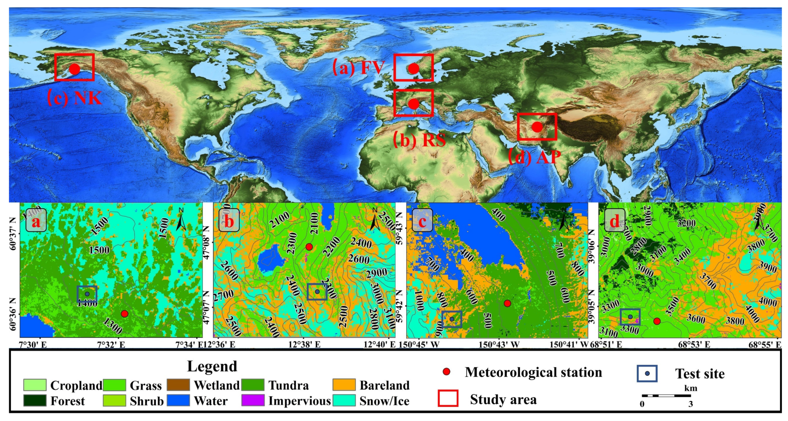
As this study was conducted to analyze the generalizability of the soil signal effect on the correlation between CR and SD, typical thick snow (Maximum SD around 100 cm) study areas located in the Northern Hemisphere were selected. The four selected study areas were in Norway, Austria, the United States, and Tajikistan with mean air temperatures of approximately −0.36 °C, 0.77 °C, 3.38 °C and −1.07 °C, respectively, from 2017–2019, and with snow accumulation period generally extending from October to March of the following year. Figure 1 shows the distribution of land-cover types and contours in the four study areas. Each study area is in a high mountainous region, and the land type consists mainly of bare soil (rock or soil with very sparse vegetation for the entire year) and low vegetation (tundra or grassland). The meteorological station provides complete and recent data, the details of which are given in Table 1, specifically including the station latitude and longitude, elevation, and land-cover types at the observation site. In addition, each study area covers an area approximately 5 × 5 km2 in size, and the topography around the meteorological observation sites is relatively flat.

Figure 1.
Land-cover types—derived from the Finer Resolution Observation and Monitoring of Global Land Cover (FROM-GLC10) data product—and contour distribution of four typical thick snow study areas located in the Northern Hemisphere: (a) FV; (b) RS; (c) NK; (d) AP. The locations of the meteorological stations and test sites (used for correlation analysis) are also shown for each study area. The global distribution of the location of each study area is shown in the background map (provided by NOAA’s ETOPO1 data).

Table 1.
Detailed information on the four meteorological stations selected on a global scale, including their continents, countries, names, locations, and land-cover types.
2.2. Data
2.2.1. Sentinel-1 Data
The data was derived from the Sentinel-1 satellite with a dual-polarized C-band synthetic aperture radar—a satellite system consisting of two satellites in the same near-Earth orbit with a phase difference of 180°—which provide global data from 2014 to the present [31]. The Level-1 Ground Range Detected (GRD) data product is used in this study, which contains both VV and VH polarizations acquired in Interferometric Width Swath mode (IW), and the pixel spacing of the image is 10 m × 10 m. Compared to Single Look Complex (SLC) data, GRD data products do not contain phase information, but the amount of data is smaller in comparison. In addition, we used the GEE platform to download and process GRD data in order to improve the timeliness of data processing. Table 2 provides the image data acquisition mode for the study area and the number of images for each orbit at different flight directions between November 2016 to March 2020. The temporal resolution of the data before 2016 is inadequate, as the Sentinel-1B commissioning phase was completed on 16 September 2016.
Table 2.
Image acquisition mode and the number of images from different satellites (Platform) in different orbits (ascending and descending) for the four study areas between November 2016 and March 2020.
There were deviations in the scattering values of images acquired by the satellite in different flight directions and different orbits due to the angle of incidence. Although some studies have proposed merged algorithms for ascending and descending orbits data, they have been tested and do not work well in the study areas of this paper [10,11]. Our study focuses on highlighting snow phenological information from the temporal evolution of feature area values; therefore, to avoid biased values in the time series as much as possible, we chose data from the same flight direction and the same orbit. After testing the data from the four study areas, it was found that there were more images from ascending orbits than from descending orbits and that there were fewer outliers in the time series. Therefore, we used ascending orbit data from Sentinel-1, and the corresponding satellite orbit number for the four study areas are 44, 44, 65, and 71, respectively.
2.2.2. Land-Cover Type Product (FROM-GLC10) and Google Earth Images
The global land-cover types, with a spatial resolution of 10 m, were provided by the Finer Resolution Observation and Monitoring of Global Land Cover (FROM-GLC10) data product [32]. In this study, the FROM-GLC10 product in 2017 was classified into ten categories: crop, forest, grass, shrub, wetland, water, tundra, impervious, bare land, and snow/ice, as the auxiliary information to study CR variation of different land types.
For further discriminating the land type, color Google Earth images save as jepg files were used. The images were provided by Maxar Technologies and CENS/Airbus. Although the image of Google earth has a high-spatial resolution, it only contains three channels of RGB and no spectral information.
2.2.3. Meteorological Data
The snow depth and average air temperature data of the meteorological station were downloaded from the National Oceanic and Atmospheric Administration (NOAA), which includes many climatology networks, such as the GHCN-Daily, WMO, and CoCoRaHS [33,34]. The data were pre-processed and delivered on a daily time scale. In this study, we used the daily snow depth and average air temperature from November 2016 to March 2020 as auxiliary information to match the Sentinel-1 data.
2.2.4. DEM Data
To perform radiometric slope correction, we constructed the terrain geometry for the study area using the digital elevation model (DEM) data, which ideally should have the same resolution as the Sentinel-1 image [35]. In this study, DEM information is derived from the ASTER GDEM V3 (Advanced Spaceborne Thermal Emission and Reflection Radiometer Global Digital Elevation Model) dataset with a spatial resolution of 30 m [36].
3. Methods
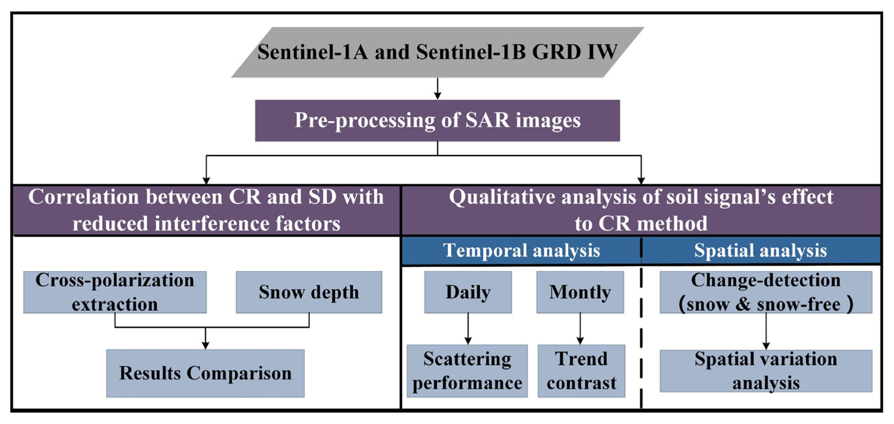
The GRD data from Sentinel-1 was used as main input. The overall workflow of the study is outlined in Figure 2, and consists of three blocks: (a) pre-processing of SAR image data; (b) correlation analysis between CR values and SD with reduced disturbing factors; (c) qualitative analysis of the effect of the soil signal on the CR method.

Figure 2.
Overall workflow for exploring the backscattering properties of feature areas under snow cover using Sentinel-1 data in GEE.
3.1. Pre-Processing of SAR Images
The GRD dataset in the GEE has been processed by the Sentinel-1 Toolbox(S1TBX) provided by the European Space Agency (ESA), including applying orbit file, removing thermal noise, removing GRD border noise, radiometric calibration, and Range-Doppler terrain correction. The final data were converted to dB by 10*log10 σ°.
The study areas are mostly located in mountainous thick snow areas, and the terrain is rugged and complex. Therefore, in order to analyze the variation of the backscatter during the snow period, we performed radiometric slope correction of SAR images according to the processing specification proposed by the Committee on Earth Observation Satellite (CEOS) [37]. The correction uses an angular-based method, the principle of which is shown in Figure 3, which removes geometric and radiometric distortions caused by topographic factors. We used equation proposed by [38] for optimizing snow volume scattering, expressed as follows:
where represents the incident angle, represents the corrected backscatter values, and can be defined as follows:
where is slope aspect angle, is the look direction, and is the slope steepness.
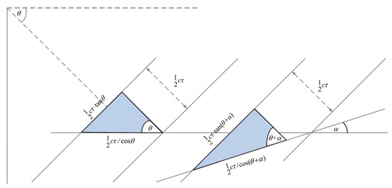
Figure 3.
Angle-based radiometric terrain correction principle: The left triangle is the flat terrain and the right triangle is the steep slope (the angle is α). The incidence angle θi equals 90° − θ. The range resolution is (where c is the speed of light, and is the pulse duration).
We followed the approach presented in [35] for masking the invalid data, as well as the layover, shadow regions in SAR images, which has been implemented in the GEE platform and is easily adaptable to other SAR missions.
3.2. Correlation between CR and Snow Depth with Reduced Disturbing Factors
The CR method, proposed by [28], uses the strong correlation between the ratio of VH and VV (cross-polarization ratio; CR) and SD to construct the snow index, then obtains a generally applicable empirical formula after rescaling the index using the measured SD data. For SAR images with high spatial resolution, whether the correlation between CR and SD is better than a single polarization is the foundation for constructing the retrieval algorithm. In order to reduce the disturbing of factors other than snow in the signal and highlight the contribution of SD in the evolution of the time-series, an area located near the meteorological station with a rocky surface was selected as a test site in each study area (Figure 1). The reason for this choice is that the rocks have less soil moisture, and, therefore, less variation in the soil dielectric constant. To ensure the applicability of the SD data, we selected test sites within 1 km of the meteorological station, which was at a similar elevation to the meteorological station. Finally, we compared the variation of VH, VV, CR, and SD in the temporal variation at the daily timescale, and calculated the Pearson correlation between CR and SD.
3.3. Qualitative Analysis of Soil Signal’s Effect to CR Method
3.3.1. The Rules for Feature Areas Selection
We defined two land types as feature areas in each study area, including rock areas (represented by boulder and bedrock) and soil areas (represented by sparse vegetation such as grassland and tundra). Based on the land-cover types provided by the FROM-GLC10 product with a spatial resolution of 10 m, we used high-resolution Google Earth images for further visual interpretation. We first excluded the forest areas, and then delineated the specific locations of the sampling points using manual interpretation. Rock areas are mainly located in Snow/Ice and Bare areas, while soil areas covered by sparse vegetation are mainly in Tundra, Grass, and Shrub. We selected 10 samples for each type. Besides, each sampling point was as close as possible to each other and at a similar elevation in order to make the CR values of the feature points more representative. Expressly, we set 60 m as the scale when processing the CR values of a single point in GEE. The purpose of this setting is to match the spatial resolution of the DEM data (30 m) used in the radiometric slope correction. Since the adjacent image elements have some influence on the value of the sampling point, we extended the distance by half an image element around the range of a single image element, as the size of the sampling points.
3.3.2. The Daily Timescale Comparison of CR Scattering Performance for Different Feature Areas
To qualitatively study the effect of the soil signal on C-band CR signals, we compared the temporal evolution of CR for different types of features at the daily timescale. Specifically, we calculated CR values for each feature areas separately in the study areas for the period November 2016–March 2020. In order to make the CR values of each feature type more homogeneous and representative, we averaged the values of 10 samples as the ultimate result. In addition, time-series of CR describe the process of change in feature areas over time, and are inevitably contaminated by many factors, which can cause biases. The Savitzky–Golay (SG) filter is a widely used time-series reconstruction model [39]. In this study, we used the SG filter to smooth the values of the CR in order to highlight snow phenological information.
3.3.3. The Monthly Timescale Analysis of Variation Characteristics for Different Feature Areas
Compared with the daily timescale variation, the values on the monthly timescale showed a more stable variation pattern, which facilitated our quantitative analysis of the soil signal’s effect. Specifically, to analyze the scattering characteristics of different feature areas on a monthly timescale, we averaged the monthly Sentinel-1 observations and analyzed the CR values from October to March of the following year, which are the main months of snow accumulation. In addition, we performed a trend analysis using monthly average CR values for the snow accumulation period.
3.3.4. Analysis of Spatial Variation at the Time of Peak Snow Accumulation
In this study, the Image-Differencing method was used to calculate the spatial variation of peak snow months. This method is commonly used in remote sensing images as one of the change detection methods. The variation for each location l and monthly time step t can be expressed as follows:
where represents the combination of VH- and VV-polarization observations (in dB), of the general form:
Specifically, the snow-free and snow-covered images used in the change-detection analysis were obtained by averaging the CR values over images of one month in the region. In addition, to further calibrate the spatial variation of the backscatter caused by snow accumulation, the following processing was used in this study: (a) to remove speckle noise, we performed a focusing operation on the images in GEE. We used three pixels as the radius of the neighborhood range and replaced the values of the other image elements in the domain with the range’s median values, for snow-free as well as snow-covered CR images, respectively, before proceeding with the change-detection method; (b) to highlight the CR changes caused by snow accumulation and filter out the outliers, we set a threshold and masked the images beyond it. The suitable threshold was obtained by comparing statistical pixel values in the study area with contemporaneous optical data; (c) to further visually highlight snow in the image and distinguish it from the masked areas in the pre-processing step, we used the Canny edge detector as a visual aid, thus locating strong intensity changes in the image and using blue as the boundary of the snow.
3.4. Evaluation Indexes
3.4.1. Correlation Evaluation
To quantitatively assess the relationship between SD and CR, we used the Pearson correlation coefficient to assess the correlation between these two parameters. In addition, we calculated the correlation between soil area’s CR and air temperature to determine the effect of the soil signal. In this study, the specific parameters include SD, air temperature, and the monthly CR backscatter values of rock and sparse vegetation-coved soil areas. In addition, we classified the correlations into five classifications, as shown in Table 3.
Table 3.
Rules of correlation classification.
3.4.2. Trend Test
The Mann–Kendall (M–K) method is a non-parametric test for monotonic trends, which has the advantage of not following a particular distribution and is rarely disturbed by outliers [40,41]. Based on these advantages, it has been widely used in trend analyses. In the M–K test, the Theil–Sen method is used to calculate the slope of the M–K trend, where a positive slope indicates an increasing trend, while a negative slope indicates a decreasing trend, and the absolute value of the slope reflects the strength of the trend. We also calculated p-values to describe the significance level, with p below 0.1, 0.05, and 0.01 indicating that the significance tests of 90%, 95%, and 99% were passed, respectively.
4. Results
4.1. Quantitative Relationship between CR and Snow Depth with Reduced Disturbing Factors
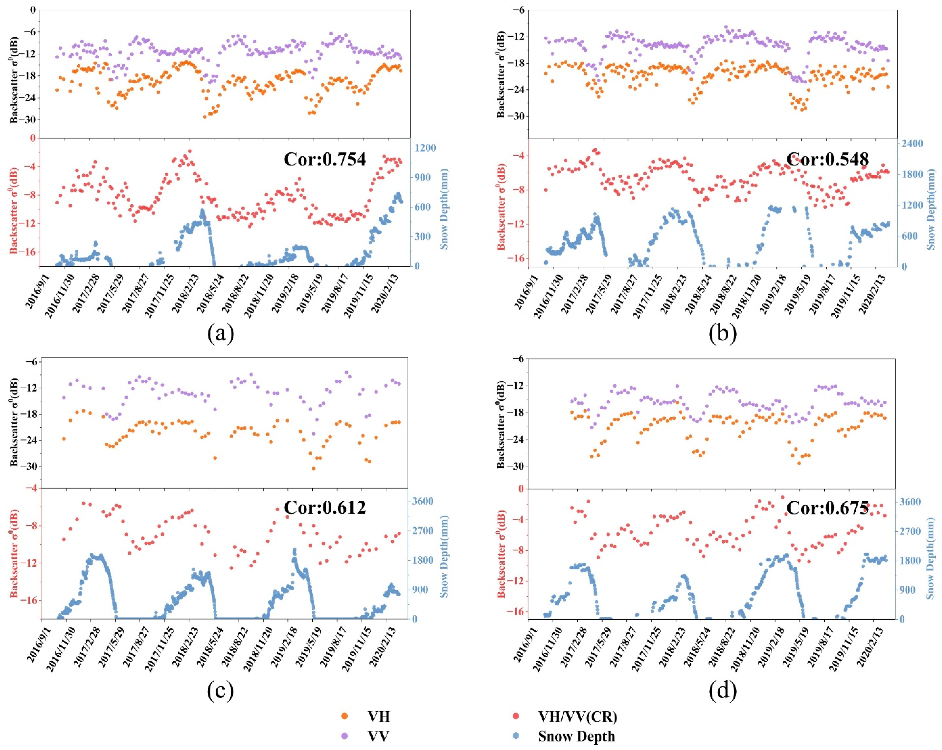
As shown in Figure 4, it is the comparison of CR, VV, VH and corresponding SD data provided by the meteorological station in the test area from November 2016 to March 2020. CR for the four study areas show a stronger correlation with SD in the temporal evolution compared to a single-polarization (VH, VV). Specifically, for VH and VV, the values of both decrease significantly from early September to the end of October each year; starting in early November, they gradually increase with the accumulation of dry snow. Interestingly, the change in VH (dB) is faster and more pronounced than the change in VV (dB). Subsequently, it can be observed that both VH and VV reach their peak around the beginning of March and no longer increase with SD. Notably, both values show a sharp decrease in early spring with the rapid melting of the snow, followed by a rapid rise and an increasing trend between May and August. In contrast, CR (dB) were better correlated with SD during the snow period, with its value showing a better upward trend as the accumulation of dry snow in early winter, peaking around the beginning of March and then dropping sharply. In addition, we calculated the correlation between CR and SD between the beginning of October and the end of February for the four study areas, which were 0.754, 0.548, 0.612, and 0.675, respectively. Note that this was the period of snow accumulation, and the snow state was dry.
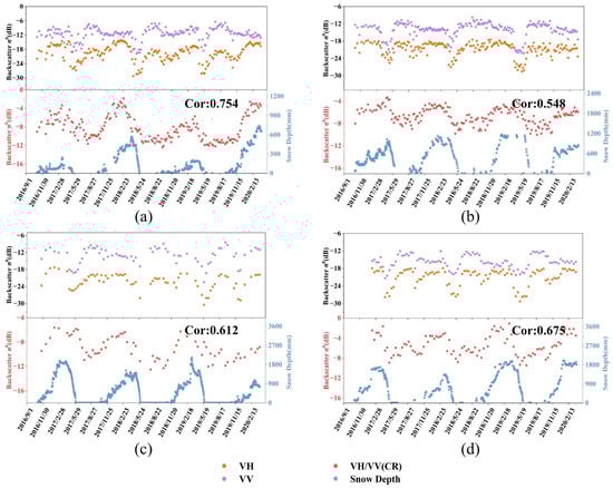
Figure 4.
Comparison of daily VH, VV and VH/VV(CR) values with SD provided by the meteorological station: (a) FV; (b) RS; (c) NK; (d) AP. Backscatter values from the same orbit of Sentinel-1 ascending data. Some outliers in the data were removed.
4.2. Qualitative Analysis of Soil Signal’s Effect to CR Method
4.2.1. Scattering Performance of Daily Timescale for Different Feature Areas
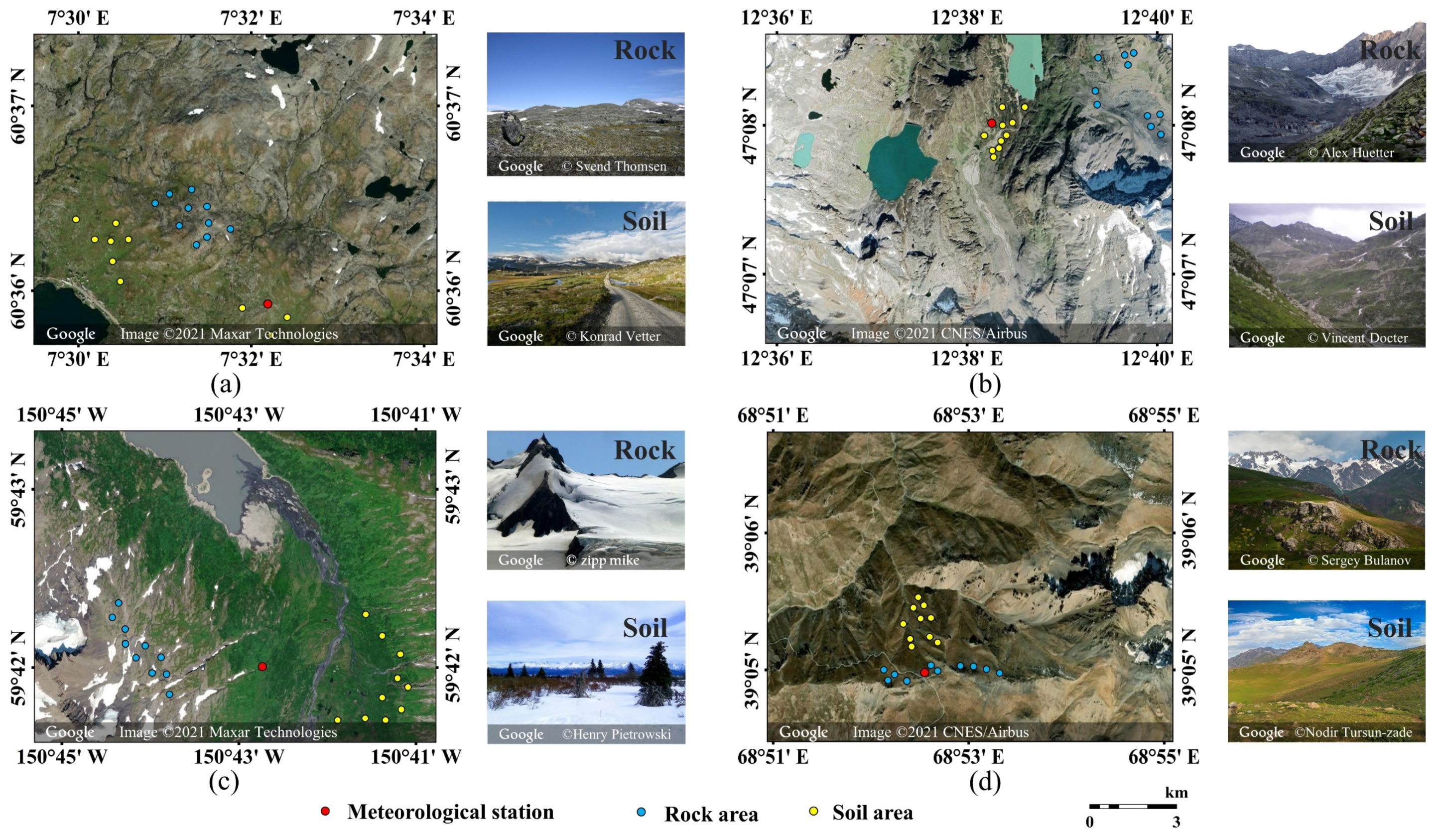
Figure 5 shows the specific locations of two types of feature areas within the four study areas. It is worth noting that one single point area may not adequately represent the behavior of a class of feature areas. The sampling points were divided into two groups, and, according to the feature areas selection rule, we respectively selected 10 sampling points in rock and soil areas of each study area, and the values of their CR were averaged as the scattering behavior of the one class of features.

Figure 5.
The specific locations of two types of feature areas within the four study areas: (a) FV; (b) RS; (c) NK; (d) AP. The blue represents rock areas, while the yellow represents soil areas. Color images and photos of the corresponding feature areas are from Google Earth Pro.
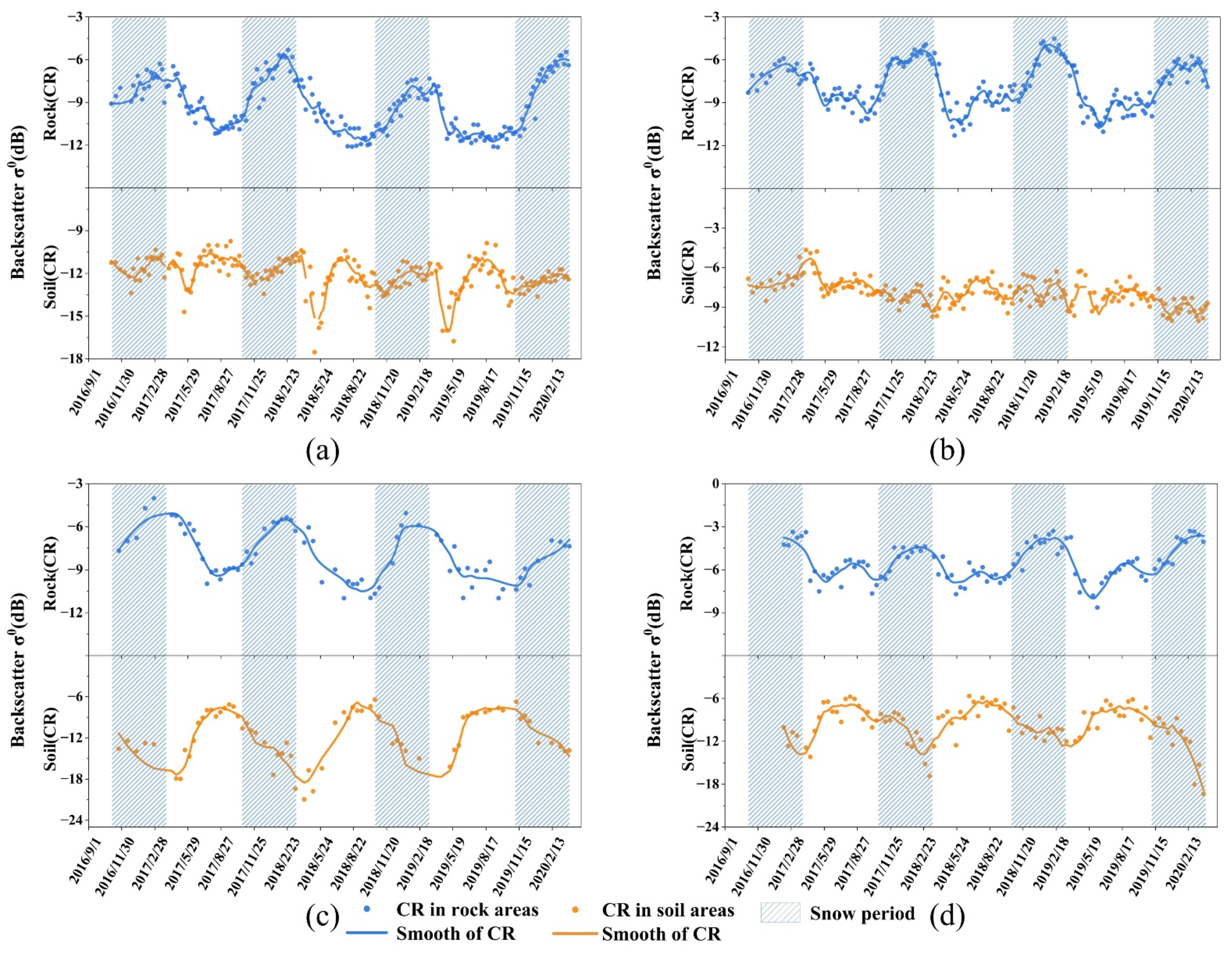
Figure 6 presents a time-series comparison of CR signals on the daily timescale for rock and sparse vegetation-covered soil areas in the four study areas from November 2016 to March 2020. For rock areas, CR in all four study areas exhibited sensitivity to snow accumulation. In particular, CR values showed a significant increase during the snow period from November to February each year and a rapid decrease from the snowmelt period in early March. However, this phenomenon was not evident in soil areas. In FV and RS, CR values showed an increase only in the middle of the snowpack period, and the trend was not obvious (Figure 6a,b). Moreover, the CR even showed a negative correlation with snow accumulation in the soil areas throughout the snow period in NK and AP.

Figure 6.
Time series of CR values for the two types of feature areas at the daily timescale during November 2016 to March 2020. Data smoothed by Satitzky-Golay filter (Points of Window is 10). (a) FV; (b) RS; (c) NK; (d) AP.
4.2.2. CR Temporal Evolution at Monthly Timescale and Trend Analysis
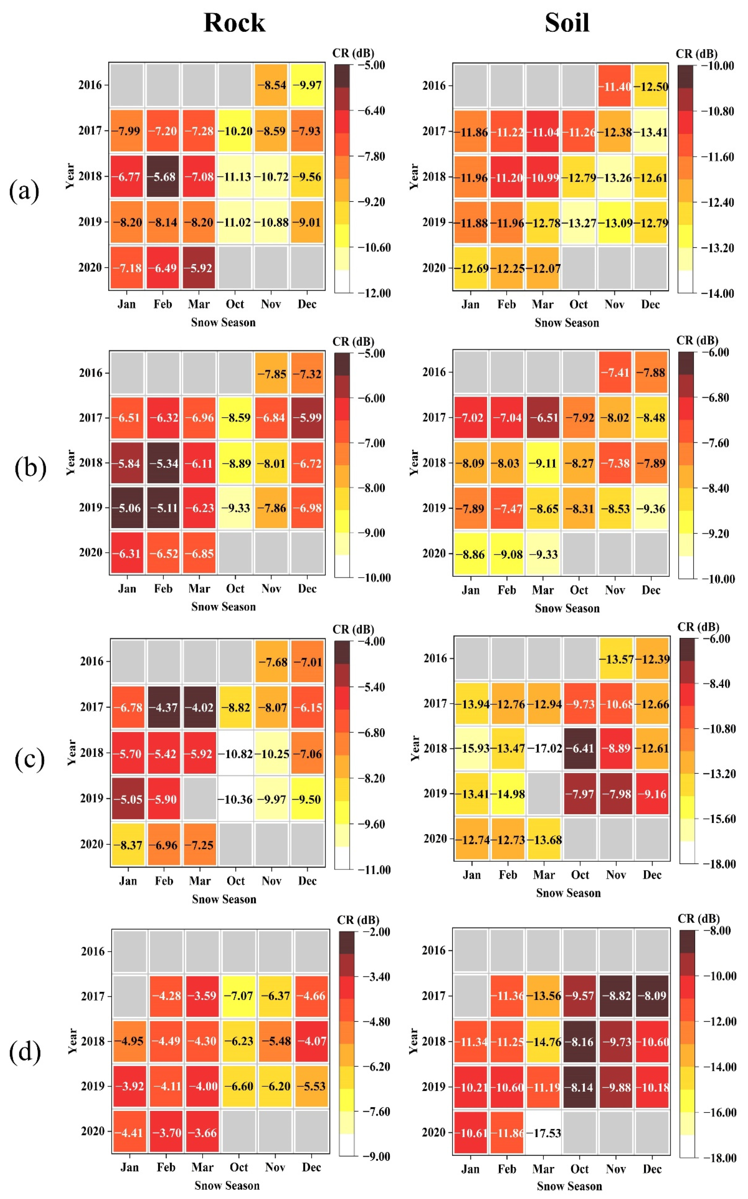
As shown in Figure 7, we averaged CR of each month for rock and sparse vegetation-covered soil areas during the snow accumulation period (October to March of the following year) from 2016–2020, in order to obtain the CR variation characteristics at a monthly time scale. During the annual snow season, the CR values in rock areas of all four study areas showed a significant increase in November and, peaked in February or March, consistent with the change in SD obtained from meteorological station observations. In contrast, CR values for soil areas covered by sparse vegetation during the snow season showed an increasing trend only in some years in FV and RS. Still, the change was not significant, such as from −11.40 to −11.04 in FV and from −7.41 to −6.51 in RS during the 2016 snow season. Besides, CR values for soil areas during the snow period showed a negative trend in NK and AP. More specifically, CR of NK peaked in October of each year with values of −9.73, −6.41, and −7.97, respectively, and then began to decrease. Similarly, the same phenomenon was observed in AP, where the peak of CR values between 2017 and 2019 occurred in October or November, with values of −8.82, −8.16, and −8.14, respectively.
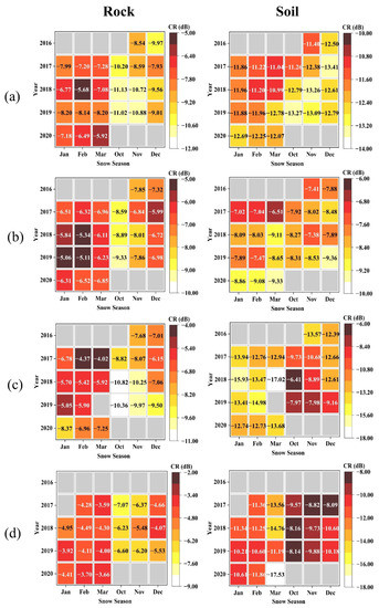
Figure 7.
Monthly CR variations for four typical study areas during the snow season (October to March of the following year) between 2016 and 2020. Gray blocks represent no available data: (a) FV; (b) RS; (c) NK; (d) AP.
In addition, we analyzed the trends in CR values for the two types of feature areas on monthly time scale during the snow period. Table 4 shows the results of the CR trend test during the snow period (October to March) from 2016 to 2020. Specifically, for the study area FV, the CR values of both types of feature areas showed an upward trend during the snow period, but the upward trend for rock areas (Slope = 0.40, 0.97, 0.71, 1.13; p = 0.22, 0.06, 0.06, 0.01) was significantly stronger than that of soil areas (Slope = 0.30, 0.21, 0.21, 0.24; p = 0.22, 0.26, 0.26, 0.01), and CR of rock areas passed the 90% significance test for most years. For RS, the CR of rock areas also showed an upward trend (Slope = 0.36, 0.49, 0.87, 0.49, p = 0.22, 0.13, 0.13, 0.13), but it did not pass the significance test; soil areas showed a negative or no trend (Slope = 0.24, −0.11, −0.03, −0.20; p = 0.22, 0.13, 1, 0.13). For both NK and AP, there was an upward trend in rock areas (NK: Slope = 0.95, 0.58, 1.67, 0.68; p = 0.03, 0.06, 0.09, 0.02; AP: Slope = 0.55, 0.44, 0.67; p = 0.02, 0.13, 0.01) and a negative trend in the soil areas (NK: Slope = −0.01, −1.46, −2.20, −1.19; p = 1, 0.02, 0.03, 0.02; AP: Slope = −1.04, −0.89, −1.02; p = 0.26, 0.06, 0.01), and the CR of rock passed the 90% significance test.
Table 4.
Results of Mann–Kendall trend test performed of monthly-scale CR for two types of feature areas during the snow accumulation season (October to March of the following year).
4.2.3. CR Spatial Variation Characteristics at the Time of Peak Snow Accumulation
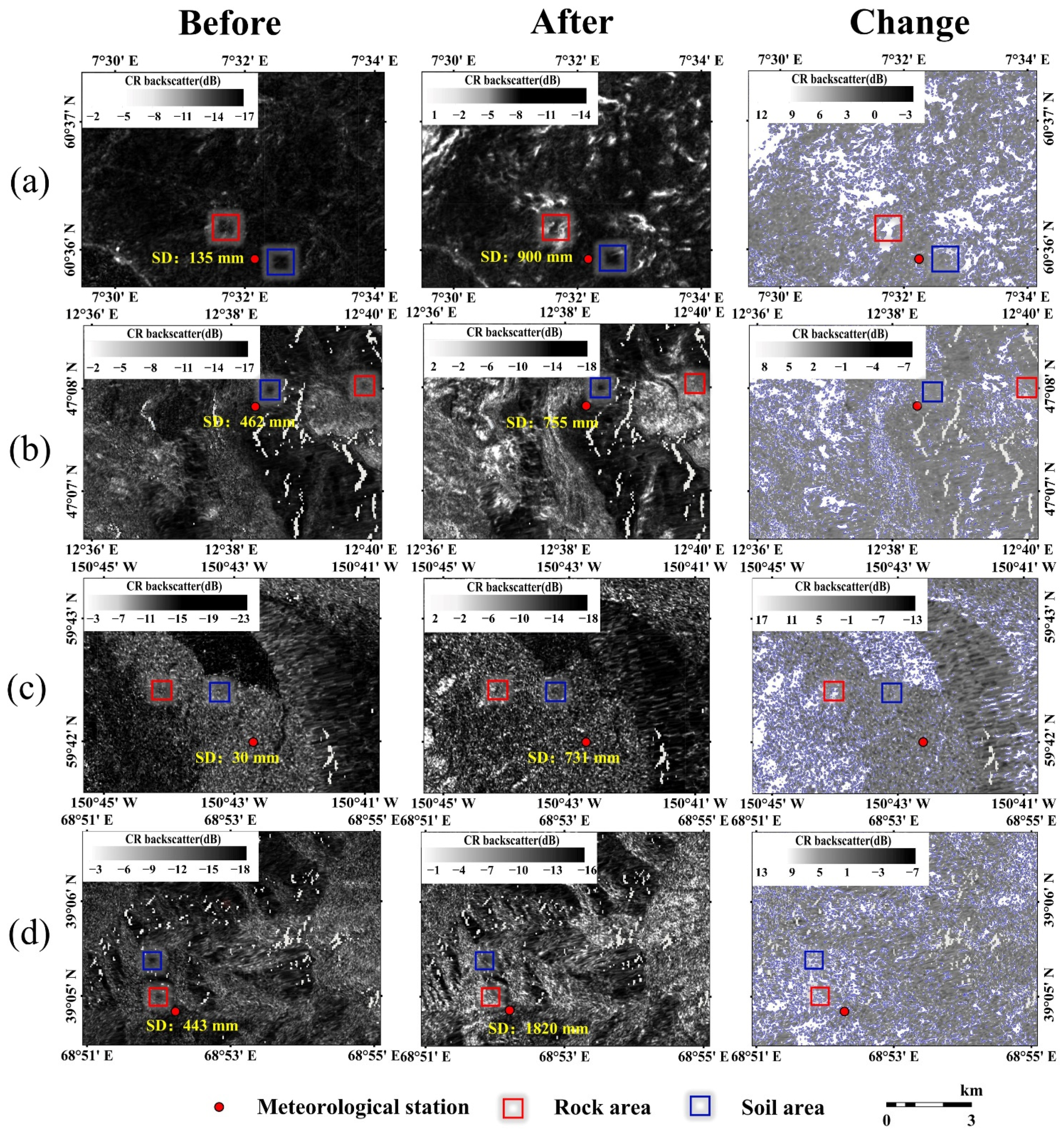
To assess the effect of soil on the correlation between C-band CR values and SD, we visually compared Sentinel-1 satellite CR-band images of the four study areas before and after the peak snow accumulation. As shown in Figure 8, each area included three images: the ascending CR-band images of before (November 2019) and after (February 2020) snow accumulation, as well as change difference obtained by using the change-detection method. It should be noted that the images before and after the peak snow accumulation were obtained by averaging the values of the CR of one month’s images of the region. Typically, the CR value at the peak of the snow accumulation was higher than that in the image without snow; that is, the images exhibited higher brightness overall. In our results, the images in February were significantly brighter than those in September. Furthermore, after comparing the change difference images with the land-cover and elevation distribution of the study area (Figure 1), we found that the variation in CR was more pronounced when the land type was rock and at higher elevations. At the same time, the yellow numbers around the observation site of the meteorological station in Figure 8 show the average SD for the month; however, even when the average SD was around 1000 mm, the variation caused by snow around the meteorological station was not significant.
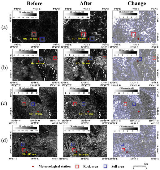
Figure 8.
The CR-band images before and after the peak snow accumulation month and the difference map obtained by the change-detection method The left and middle columns show the monthly mean CR maps for November 2019 and February 2020, while the right column shows the CR variation caused by snow accumulation, which was obtained by image processing. The red boxes represent the rock areas, and the blue boxes represent the soil areas covered by sparse vegetation. The red point indicates the location of the meteorological station and next to it is the average SD (marked in yellow). (a) FV; (b) RS; (c) NK; (d) AP.
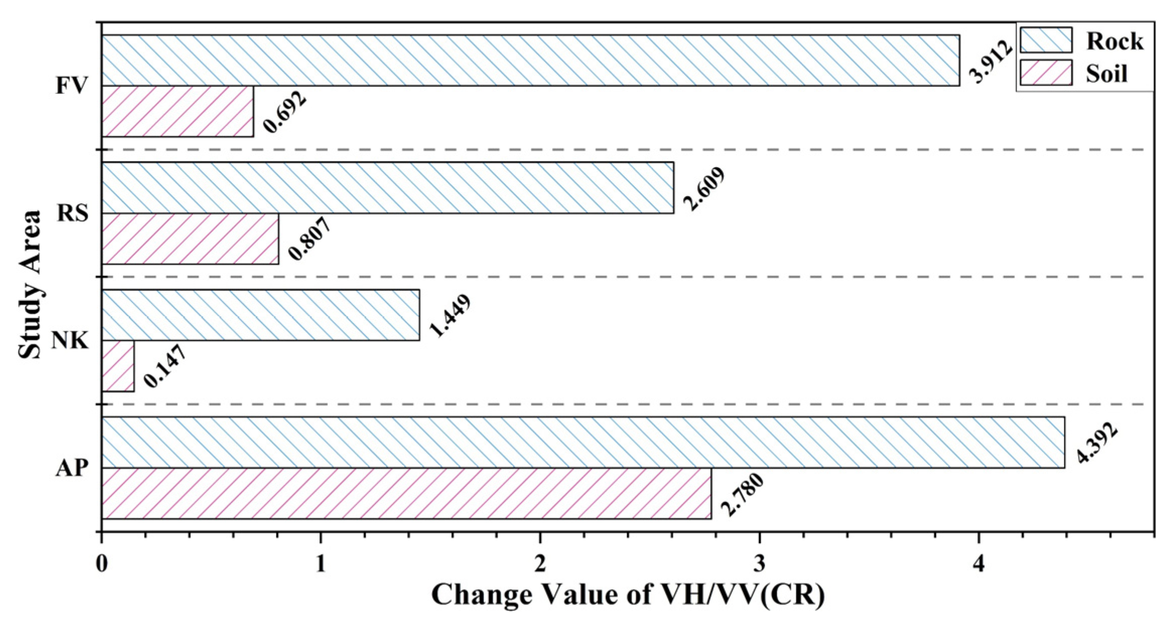
Although each study area was small and contained meteorological stations (ensuring a deeper winter snow thickness within the area), we found that not all areas within the study area significantly increased in brightness. Based on the land-cover types provided by the FROM-GLC product and the high-spatial-resolution optical images provided by Google Earth, we selected rock areas (red boxes) and soil areas (blue boxes), as shown in Figure 8, where the land types are distinct and the topography is flatter, compared to other locations. As shown in Figure 9, we compared the specific differences between the two of them. The results show that the variation of the monthly average CR after snow accumulation is more pronounced in rock areas, with variation difference values of 3.912, 2.609, 1.449, and 4.392 in the four study areas, respectively, which are several times higher than those in soil areas covered by sparse vegetation. Therefore, we speculate that, although the CR method based on Sentinel-1 data quantitatively distinguishes snow volume scattering from soil surface scattering to a certain extent, for high spatial resolution (30 m) data, the backscatter values are still dominated by the soil signal in areas with high water content.

Figure 9.
Comparison of monthly mean CR change values in rock and soil areas (November 2019 and February 2020).
5. Discussion
5.1. Physical Mechanisms of Different Polarization Modes to Snow Scattering When There Are Few Disturbing Factors
As shown in the results of Section 4.1, for SAR images with high spatial resolution, the CR of Sentinel-1 has a better correlation with the SD under conditions with fewer disturbing factors, compared to the single polarization mode VH and VV. Furthermore, the value of VH undergoes a significant increase with increasing SD during the snow period, while VV changes less, so the ratio of VH to VV (CR) better reflects the changes in SD. The explanation based on the physical mechanism is that the snow causes vertically emitted polarization (V-polarized) waves to scatter multiple times on the ground, thus changing the electric field vector of part of the V-polarized wave, such that the horizontal receiving channel of the radar has more opportunities to receive the echoes (H-polarized). As the thickness of the snow increases, the path length of the V-polarized wave through the snow increases so that the electric field vector of the wave has a greater chance to change [42]. Afterwards, as the temperature rises in the spring, the liquid water in the wet snow causes a strong absorption of electromagnetic waves, such that both VH and VV show a sharp decrease. After the complete melting of the snow, the echo signal on the ground is again dominated by the soil signal, and shows an upward trend.
5.2. Uncertainties Affecting the Backscatter
5.2.1. Effect of Soil Surface Freeze-Thaw Cycles
Backscatter is determined by a combination of sensor factors and ground conditions [43]. With constant sensing element parameters, such as frequency and polarization, the variation of backscatter is caused exclusively by surface parameters, vegetation structure, and snow accumulation. In addition, soil roughness and soil moisture determine the soil signal. Therefore, for a single scattering surface covered with snow, soil moisture and snow are the main factors affecting backscattering, as the soil roughness remains constant in winter [16]. The results in Section 4.1 demonstrated that there is a significant decrease in both VH and VV in early winter, due to the soil freeze-thaw cycle. In early winter, the temperature gradually drops and the soil surface starts to freeze, causing water molecules to accumulate in the lattice, which will cause a rapid decrease in the soil dielectric constant, in turn causing the backscatter value to decrease [44]. Subsequently, the stabilization of the soil freezing fraction and the gradual increase in the volume scattering of snow on the soil surface led to a better correlation between CR and SD [45,46].
Although the CR method can eliminate the influence of system parameters and environmental factors on snow volume scattering to some extent, scattering results in soil areas covered by sparse vegetation show that the soil surface scattering still disturbs the correlation between SD and CR signal, thus affecting the retrieval results. The results of Section 4.2 demonstrate that the correlation between CR and SD in soil areas is low, or even shows a negative correlation. A reasonable explanation is the higher water content of the soil area and that the C-band can easily penetrate dry snow (penetration depth of about 10 m when the snow density is 200 kg m−3 [47]). Therefore, the snow volume contributes less to the total scattering signal, compared to the scattering from the soil surface [48,49].
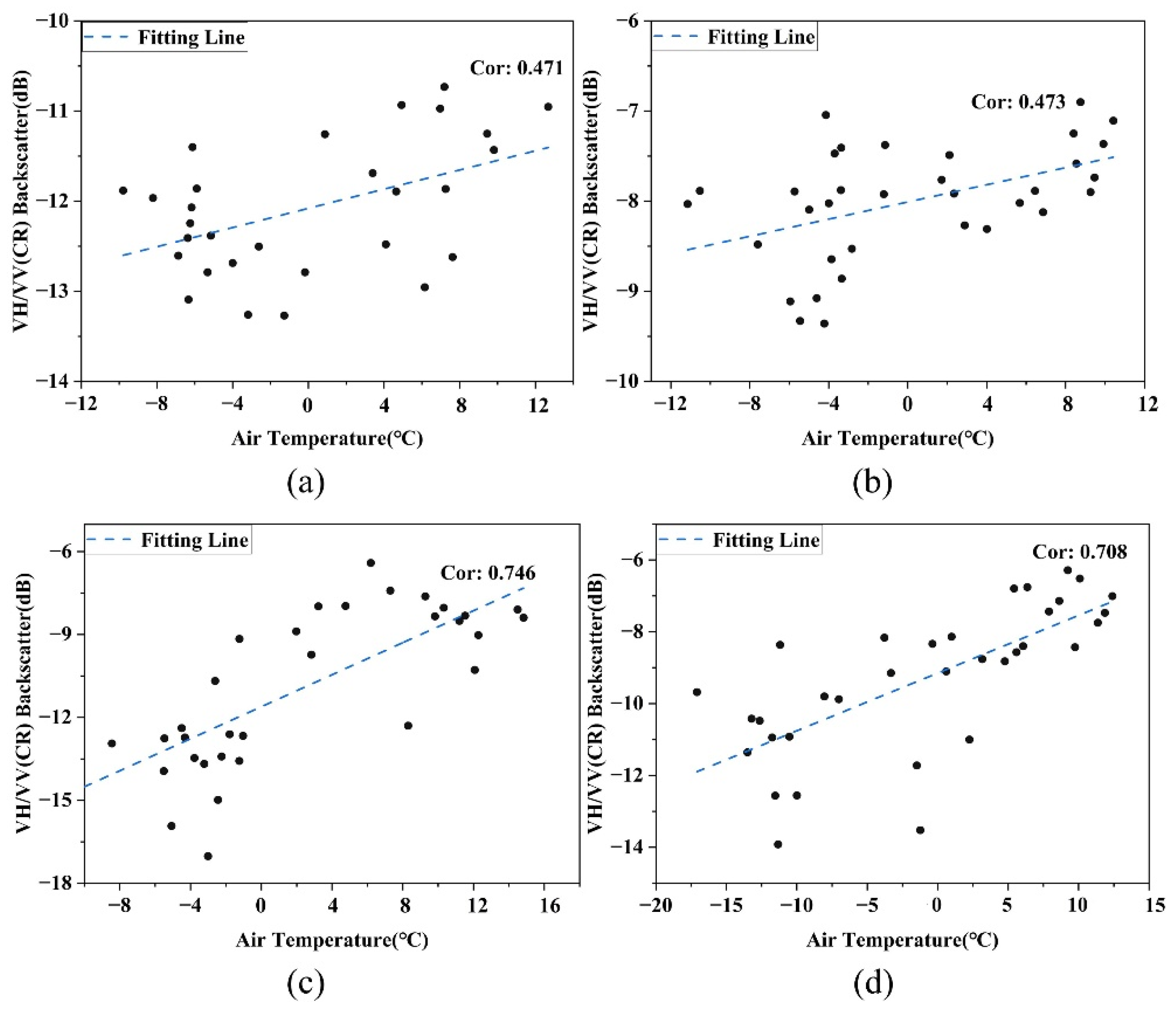
Figure 10 shows the correlation between CR and air temperature at monthly time scale for the four study areas. We excluded data for snowmelt months based on SD data from the meteorological station, as liquid water on the surface of wet snow absorbs the signal and, thus, affects the scattering mechanism of the radar. For the study areas NK and AP, there was a strong Pearson correlation between CR and air temperature (0.746 and 0.708, respectively). In contrast, the FV and RS showed a moderate correlation of 0.471 and 0.473, which can be attributed to the low moisture content of the feature areas. In addition, some studies have suggested that the total backscatter increases with SD as the temperature decreases and the soil reaches the point of complete freezing, for a completely frozen surface is the same as the rock area, and they both have relatively stable dielectric constants [44,50,51]. We also observed this phenomenon in research, where the SD increased from November in the soil areas of the FV and RS, but the corresponding CR values did not change much, and significant changes were not observed until February.
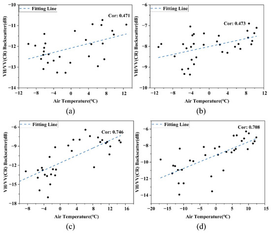
Figure 10.
Pearson correlation coefficients between monthly scale air temperature (℃) and CR values (dB) for soil areas in the four study areas: (a) FV; (b) RS; (c) NK; (d) AP.
5.2.2. SAR Flight Direction (Ascending and Descending Orbits)
There are biases between different orbits (ascending/descending) of Sentinel-1 data, leading to uncertainties in retrieving the surface state. Sentinel-1 is a right-looking satellite; i.e., the side-viewing antenna is at a 90° angle to the sensor flight path, and the incidence angle of data acquired in different flight directions and orbits is different, which can lead to different backscatter values [52]. Figure 11 shows the difference between each month’s CR values of the ascending and descending orbits from October 2019 to March 2020 for the four study areas. The CR value is obtained by calculating the monthly average CR’s difference between each month (October 2019–March 2020) and September 2019 (snow-free). We note that the different flight directions may lead to various variation differences in the backscatter values for the study areas except FV and RS, which were caused by the number of images in the study area and the topographic conditions of the area. Therefore, merging ascending and descending orbit data is challenging in different heterogeneous environments [10]. Many studies have normalized SAR data to the same incidence angle, thus achieving data merging with a view to reducing the observation period of the data [53]. In terms of incidence angle, a smaller incidence angle (>35–40°) increases the depth through the snow and maximizes the scattering contribution from the snow; while, when the incidence angle is steeper (<30°), it reduces the attenuation and makes the contribution from ground scattering in the signal more pronounced [54].
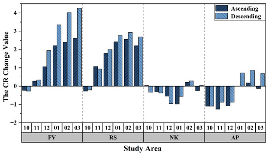
Figure 11.
The monthly CR value difference between each month of 2019 snow season (October 2019–March 2020) and September 2019 for the ascending and descending orbits at the four typical study areas.
5.3. Limitations
In this study, we quantitatively evaluated the applicability of the CR method in different feature areas, but we did not well solve the problem of soil signal disturbing. The C-band has strong penetration for dry snow, making it difficult to show obvious snow phenological information in the time evolution of CR within soil areas, even in the mountainous areas with thick snow. Therefore, establishing the relationship between SD and CR of Sentinel-1 at the high spatial resolution to achieve basin-scale SD retrieval is still a challenge. In addition, we only used data from the same flight direction and the same orbit, which would reduce the time resolution of the data. However, after testing existing fusion methods, it is found that there is still an enormous bias value in the time series of backscatter, which is not conducive to reflecting the real backscatter on the ground.
Theoretically, Sentinel-1 consists of two sensors (A and B), and the combined revisit period is 6 days, but the data obtained in different regions are different [31]. Currently, only European data coverage is complete and has a high time resolution. Therefore, for regions outside Europe, the low time resolution of Sentinel-1 may cause errors in backscatter values. Finally, the method of manual interpretation will also cause some errors when selecting feature areas. In order to identify the land type of the study area, we combined the land cover product (FROM-GLC 10) and color Google images to select two types of feature areas. However, the study area is mostly located in remote mountainous areas and lacks ground observation data, so it is impossible to directly verify the authenticity of the selection.
6. Conclusions
The existing literature has rarely utilized high-spatial-resolution C-band data to study the effect of dry snow on backscatter and quantitatively assess the soil signal’s influence on the SD retrieval. In this study, we first quantify the correlation between CR and SD at test sites with fewer disturbing factors, based on a large amount of Copernicus Sentinel-1 data from November 2016 to March 2020. Subsequently, a qualitative comparison of two types of feature areas with different moisture content in four typical thick snow study areas was carried out to assess the potential of C-band SAR data for SD retrieval.
The results indicated that the CR values of Sentinel-1 data are closely related to the SD in rock areas with low water content, compared to single VH- and VV-polarizations. Specifically, the Pearson correlation coefficients between CR and SD on a daily timescale in the four study areas during the snow accumulation period were 0.754, 0.548, 0.612, and 0.675, respectively. Moreover, at the high spatial resolution, the CR of sparse vegetation-covered soil areas showed no or negative trends during the snow accumulation period, due to the changes in soil dielectric constant caused by freeze-thaw cycles, but showed moderate or high correlation with the air temperature at the monthly timescale. Finally, by comparing the change characteristics of the images before and after the peak of snow accumulation, we found that the CR of SAR images with the high spatial resolution was still strongly influenced by the soil signal, which makes it still difficult to quantitatively distinguish snow volume scattering from the soil surface scattering when mixed image elements are fully considered. This study highlights the complexity of the physical mechanisms of snow scattering during winter processes and the influencing factors that cause uncertainty in the SD retrieval.
In future work, the study on the mechanism of various polarizations and the combination of different polarizations is a promising option, which hopefully excludes the influence of the change of soil dielectric constant in winter, so as to distinguish the snow volume scattering from the soil surface scattering. In addition, a normalization algorithm for the angle of incidence should be developed for mountainous areas, which can help to fuse ascending and descending data and thus improve the temporal resolution of the Sentinel-1 data. Finally, the grain size and density of snow will also affect the backscatter. For example, some studies have found that the backscatter would increase with SD in coarse-grained snow, but decrease in a fine-grained snow [55]. Therefore, developing SD retrieval algorithms based on fully considering the soil and snow parameters was mentioned as a crucial future development.
Author Contributions
Conceptualization, T.F. and X.H.; methodology, T.F. and X.H.; software, T.F.; validation. X.H.; formal analysis, T.F. and X.H.; investigation, T.F.; resources, J.Z.; data curation, T.F. and J.Z.; writing-original draft preparation, T.F.; writing-revies & editing, X.H., J.W., H.L., and J.Z.; supervision, J.W.; projection administration, X.H., J.W., J.Z.; funding acquisition, X.H. All authors have read and agreed to the published version of the manuscript.
Funding
This research was funded by the National Key Research and Development Program of China (Grant No. 2019YFC1510503), the National Natural Science Foundation of China (Grant No.41971325, 42171391, 41861049), the Science & Technology Basic Resources Investigation Program of China (Grant No. 2017FY100502).
Institutional Review Board Statement
Not applicable.
Informed Consent Statement
Not applicable.
Data Availability Statement
Sentinel-1 GRD data can be obtained from the ESA and Copernicus Sentinel Satellites Project using Google Earth Engine (https://developers.google.com/earth-engine/datasets/catalog/COPERNICUS_S1_GRD/, accessed on 1 April 2021). The meteorological data were obtained from the National Oceanic and Atmospheric Administration (https://www.ncei.noaa.gov/maps/daily-summaries/, accessed on 1 September 2021). The land-cover type product can be obtained from the Finer Resolution Observation and Monitoring of Global Land Cover (FROM-GLC10) (http://data.ess.tsinghua.edu.cn/, accessed on 1 September 2021).
Acknowledgments
The authors would like to thank the editor and anonymous reviewers for their valuable comments and suggestions on this article.
Conflicts of Interest
The authors declare no conflict of interest.
References
- Choi, G.; Robinson, D.A.; Kang, S. Changing northern hemisphere snow seasons. J. Clim. 2010, 23, 5305–5310. [Google Scholar] [CrossRef]
- Thackeray, C.W.; Derksen, C.; Fletcher, C.G.; Hall, A. Snow and climate: Feedbacks, drivers, and indices of change. Curr. Clim. Chang. Rep. 2019, 5, 322–333. [Google Scholar] [CrossRef]
- Hall, D.; Sturm, M.; Benson, C.; Chang, A.; Foster, J.; Garbeil, H.; Chacho, E. Passive microwave remote and in situ measurements of artic and subarctic snow covers in Alaska. Remote Sens. Environ. 1991, 38, 161–172. [Google Scholar] [CrossRef]
- Xiao, X.; Zhang, T.; Zhong, X.; Li, X. Spatiotemporal Variation of Snow Depth in the Northern Hemisphere from 1992 to 2016. Remote Sens. 2020, 12, 2728. [Google Scholar] [CrossRef]
- Singh, P.; Haritashya, U.K.; Kumar, N. Meteorological study for Gangotri Glacier and its comparison with other high altitude meteorological stations in central Himalayan region. Hydrol. Res. 2007, 38, 59–77. [Google Scholar] [CrossRef]
- Foster, J.L.; Hall, D.K.; Eylander, J.B.; Riggs, G.A.; Nghiem, S.V.; Tedesco, M.; Kim, E.; Montesano, P.M.; Kelly, R.E.; Casey, K.A. A blended global snow product using visible, passive microwave and scatterometer satellite data. Int. J. Remote Sens. 2011, 32, 1371–1395. [Google Scholar] [CrossRef]
- Shaw, T.E.; Gascoin, S.; Mendoza, P.A.; Pellicciotti, F.; McPhee, J. Snow depth patterns in a high mountain Andean catchment from satellite optical tristereoscopic remote sensing. Water Resour. Res. 2020, 56, e2019WR024880. [Google Scholar] [CrossRef]
- Shaw, T.; Deschamps-Berger, C.; Gascoin, S.; Mcphee, J. Monitoring spatial and temporal differences in Andean snow depth derived from satellite tri-stereo photogrammetry. Front. Earth Sci. 2020, 8, 579142. [Google Scholar] [CrossRef]
- Che, T.; Li, X.; Jin, R.; Armstrong, R.; Zhang, T.J. Snow depth derived from passive microwave remote-sensing data in China. Ann. Glaciol. 2008, 49, 145–154. [Google Scholar] [CrossRef] [Green Version]
- Tsai, Y.-L.S.; Dietz, A.; Oppelt, N.; Kuenzer, C. Remote sensing of snow cover using spaceborne SAR: A review. Remote Sens. 2019, 11, 1456. [Google Scholar] [CrossRef] [Green Version]
- Nagler, T.; Rott, H.; Ripper, E.; Bippus, G.; Hetzenecker, M. Advancements for snowmelt monitoring by means of sentinel-1 SAR. Remote Sens. 2016, 8, 348. [Google Scholar] [CrossRef] [Green Version]
- Takala, M.; Luojus, K.; Pulliainen, J.; Derksen, C.; Lemmetyinen, J.; Kärnä, J.-P.; Koskinen, J.; Bojkov, B. Estimating northern hemisphere snow water equivalent for climate research through assimilation of space-borne radiometer data and ground-based measurements. Remote Sens. Environ. 2011, 115, 3517–3529. [Google Scholar] [CrossRef]
- Chen, H.H.; Li, L.L.; Guan, L. Cross-calibration of brightness temperature obtained by FY-3B/MWRI using Aqua/AMSR-E data for snow depth retrieval in the Arctic. Acta Oceanol. Sin. 2021, 40, 43–53. [Google Scholar] [CrossRef]
- Dai, L.Y.; Che, T.; Xie, H.J.; Wu, X.J. Estimation of Snow Depth over the Qinghai-Tibetan Plateau Based on AMSR-E and MODIS Data. Remote Sens. 2018, 10, 1989. [Google Scholar] [CrossRef] [Green Version]
- Xiao, X.; Zhang, T.; Zhong, X.; Shao, W.; Li, X. Support vector regression snow-depth retrieval algorithm using passive microwave remote sensing data. Remote Sens. Environ. 2018, 210, 48–64. [Google Scholar] [CrossRef]
- Shi, J.; Dozier, J. Estimation of snow water equivalence using SIR-C/X-SAR. I. Inferring snow density and subsurface properties. IEEE Trans. Geosci. Remote Sens. 2000, 38, 2465–2474. [Google Scholar]
- Snehmani; Singh, M.K.; Gupta, R.; Bhardwaj, A.; Joshi, P.K. Remote sensing of mountain snow using active microwave sensors: A review. Geocarto Int. 2015, 30, 1–27. [Google Scholar] [CrossRef]
- Guneriussen, T.; Hogda, K.A.; Johnsen, H.; Lauknes, I. InSAR for estimation of changes in snow water equivalent of dry snow. IEEE Trans. Geosci. Remote Sens. 2001, 39, 2101–2108. [Google Scholar] [CrossRef]
- Liu, Y.; Li, L.; Yang, J.; Chen, X.; Hao, J. Estimating snow depth using multi-source data fusion based on the D-InSAR method and 3DVAR fusion algorithm. Remote Sens. 2017, 9, 1195. [Google Scholar] [CrossRef] [Green Version]
- Zhu, J.; Tan, S.; King, J.; Derksen, C.; Lemmetyinen, J.; Tsang, L. Forward and inverse radar modeling of terrestrial snow using SnowSAR data. IEEE Trans. Geosci. Remote Sens. 2018, 56, 7122–7132. [Google Scholar] [CrossRef]
- Xiong, C.; Shi, J. The potential for estimating snow depth with QuikScat data and a snow physical model. IEEE Geosci. Remote Sens. Lett. 2017, 14, 1156–1160. [Google Scholar] [CrossRef]
- Zhu, J.; Tan, S.; Tsang, L.; Kang, D.H.; Kim, E. Snow Water Equivalent Retrieval Using Active and Passive Microwave Observations. Water Resour. Res. 2021, 57, e2020WR027563. [Google Scholar] [CrossRef]
- Bernier, M.; Fortin, J.; Gauthier, Y.; Gauthier, R.; Roy, R.; Vincent, P. Determination of snow water equivalent using RADARSAT SAR data in eastern Canada. Hydrol. Process. 1999, 13, 3041–3051. [Google Scholar] [CrossRef]
- Sun, S.; Che, T.; Wang, J.; Li, H.; Hao, X.; Wang, Z.; Wang, J.J.A. Estimation and analysis of snow water equivalents based on C-band SAR data and field measurements. Arct. Antarct. Alp. Res. 2015, 47, 313–326. [Google Scholar] [CrossRef] [Green Version]
- Leinss, S.; Parrella, G.; Hajnsek, I. Snow height determination by polarimetric phase differences in X-band SAR data. IEEE J. Sel. Top. Appl. Earth Obs. Remote Sens. 2014, 7, 3794–3810. [Google Scholar] [CrossRef] [Green Version]
- Awasthi, S.; Kumar, S.; Thakur, P.; Jain, K.; Kumar, A. Snow depth retrieval in North-Western Himalayan region using pursuit-monostatic TanDEM-X datasets applying polarimetric synthetic aperture radar interferometry based inversion Modelling. Int. J. Remote Sens. 2021, 42, 2872–2897. [Google Scholar] [CrossRef]
- Pettinato, S.; Paloscia, S.; Santi, E.; Palchetti, E.; De Gregorio, L.; Notarnicola, C.; Cuozzo, G.; Marin, C.; Cigna, F.; Tapete, D. Multi-Frequency SAR Images for SWE Retrieval in Alpine Areas Through Machine Learning APPROACHES. In Proceedings of the IGARSS 2020–2020 IEEE International Geoscience and Remote Sensing Symposium, Waikoloa, HI, USA, 26 September–2 October 2020; pp. 2930–2933. [Google Scholar]
- Lievens, H.; Demuzere, M.; Marshall, H.-P.; Reichle, R.H.; Brucker, L.; Brangers, I.; de Rosnay, P.; Dumont, M.; Girotto, M.; Immerzeel, W.W. Snow depth variability in the Northern Hemisphere mountains observed from space. Nat. Commun. 2019, 10, 1–12. [Google Scholar] [CrossRef]
- Vreugdenhil, M.; Navacchi, C.; Bauer-Marschallinger, B.; Hahn, S.; Steele-Dunne, S.; Pfeil, I.; Dorigo, W.; Wagner, W. Sentinel-1 Cross Ratio and Vegetation Optical Depth: A Comparison over Europe. Remote Sens. 2020, 12, 3404. [Google Scholar] [CrossRef]
- Veloso, A.; Mermoz, S.; Bouvet, A.; Le Toan, T.; Planells, M.; Dejoux, J.-F.; Ceschia, E. Understanding the temporal behavior of crops using Sentinel-1 and Sentinel-2-like data for agricultural applications. Remote Sens. Environ. 2017, 199, 415–426. [Google Scholar] [CrossRef]
- Geudtner, D.; Torres, R.; Snoeij, P.; Davidson, M.; Rommen, B. Sentinel-1 system capabilities and applications. In Proceedings of the IEEE Geoscience and Remote Sensing Symposium, Quebec City, QC, Canada, 13–18 July 2014; pp. 1457–1460. [Google Scholar]
- Chen, B.; Xu, B.; Zhu, Z.; Yuan, C.; Suen, H.P.; Guo, J.; Xu, N.; Li, W.; Zhao, Y.; Yang, J.J.S.B. Stable classification with limited sample: Transferring a 30-m resolution sample set collected in 2015 to mapping 10-m resolution global land cover in 2017. Sci. Bull 2019, 64, 370–373. [Google Scholar]
- Reges, H.W.; Doesken, N.; Turner, J.; Newman, N.; Bergantino, A.; Schwalbe, Z. CoCoRaHS: The evolution and accomplishments of a volunteer rain gauge network. Bull. Am. Meteorol. Soc. 2016, 97, 1831–1846. [Google Scholar] [CrossRef]
- Jaffrés, J.B. GHCN-Daily: A treasure trove of climate data awaiting discovery. Comput. Geosci. 2019, 122, 35–44. [Google Scholar] [CrossRef]
- Vollrath, A.; Mullissa, A.; Reiche, J. Angular-based radiometric slope correction for Sentinel-1 on google earth engine. Remote Sens. 2020, 12, 1867. [Google Scholar] [CrossRef]
- Carrera-Hernandez, J.J. Not all DEMs are equal: An evaluation of six globally available 30 m resolution DEMs with geodetic benchmarks and LiDAR in Mexico. Remote Sens. Environ. 2021, 261, 112474. [Google Scholar] [CrossRef]
- Satellites, C.O.E.O. Analysis Ready Data For Land. Available online: https://ceos.org/ard/files/PFS/NRB/v5.0/Normalised_Rader_Backscatter-v5.0 (accessed on 1 March 2021).
- Hoekman, D.H. Radar Remote Sensing Data for Applications in Forestry. Doctoral Dissertation, Internally Prepared, Laboratory of Geo-Information Science and Remote Sensing, Wageningen University, Wageningen, The Netherlands, 1990. [Google Scholar]
- Zhou, J.; Jia, L.; Menenti, M.; Gorte, B. On the performance of remote sensing time series reconstruction methods—A spatial comparison. Remote Sens. Environ. 2016, 187, 367–384. [Google Scholar] [CrossRef]
- Mann, H.B. Nonparametric tests against trend. Econom. J. Econom. Soc. 1945, 13, 245–259. [Google Scholar] [CrossRef]
- Kendall, M.G. Rank Correlation Methods; Griffin: Oxford, UK, 1948. [Google Scholar]
- King, J.; Kelly, R.; Kasurak, A.; Duguay, C.; Gunn, G.; Rutter, N.; Watts, T.; Derksen, C. Spatio-temporal influence of tundra snow properties on Ku-band (17.2 GHz) backscatter. J. Glaciol. 2015, 61, 267–279. [Google Scholar] [CrossRef] [Green Version]
- Wang, L.; Qu, J.J. Satellite remote sensing applications for surface soil moisture monitoring: A review. Front. Earth Sci. China 2009, 3, 237–247. [Google Scholar] [CrossRef]
- Naeimi, V.; Paulik, C.; Bartsch, A.; Wagner, W.; Kidd, R.; Park, S.-E.; Elger, K.; Boike, J. ASCAT Surface State Flag (SSF): Extracting information on surface freeze/thaw conditions from backscatter data using an empirical threshold-analysis algorithm. IEEE Trans. Geosci. Remote Sens. 2012, 50, 2566–2582. [Google Scholar] [CrossRef]
- Bergstedt, H.; Bartsch, A.; Neureiter, A.; Höfler, A.; Widhalm, B.; Pepin, N.; Hjort, J. Deriving a Frozen Area Fraction From Metop ASCAT Backscatter Based on Sentinel-1. IEEE Trans. Geosci. Remote Sens. 2020, 58, 6008–6019. [Google Scholar] [CrossRef] [Green Version]
- West, R.D. Potential applications of 1–5 GHz radar backscatter measurements of seasonal land snow cover. Radio Sci. 2000, 35, 967–981. [Google Scholar] [CrossRef] [Green Version]
- Snehmani; Venkataraman, G.; Nigam, A.; Singh, G. Development of an inversion algorithm for dry snow density estimation and its application with ENVISAT-ASAR dual co-polarization data. Geocarto Int. 2010, 25, 597–616. [Google Scholar] [CrossRef]
- Bergstedt, H.; Zwieback, S.; Bartsch, A.; Leibman, M. Dependence of C-band backscatter on ground temperature, air temperature and snow depth in arctic permafrost regions. Remote Sens. 2018, 10, 142. [Google Scholar] [CrossRef] [Green Version]
- Widhalm, B.; Bartsch, A.; Goler, R. Simplified normalization of C-band synthetic aperture radar data for terrestrial applications in high latitude environments. Remote Sens. 2018, 10, 551. [Google Scholar] [CrossRef] [Green Version]
- Bergstedt, H.; Bartsch, A.; Duguay, C.R.; Jones, B.M. Influence of surface water on coarse resolution C-band backscatter: Implications for freeze/thaw retrieval from scatterometer data. Remote Sens. Environ. 2020, 247, 111911. [Google Scholar] [CrossRef]
- Bergstedt, H.; Bartsch, A. Surface state across scales; temporal and spatial patterns in land surface freeze/thaw dynamics. Geosciences 2017, 7, 65. [Google Scholar] [CrossRef] [Green Version]
- Panetti, A.; Rostan, F.; L’Abbate, M.; Bruno, C.; Bauleo, A.; Catalano, T.; Cotogni, M.; Galvagni, L.; Pietropaolo, A.; Taini, G. Copernicus sentinel-1 satellite and C-SAR instrument. In Proceedings of the 2014 IEEE Geoscience and Remote Sensing Symposium, Quebec City, QC, Canada, 13–18 July 2014; pp. 1461–1464. [Google Scholar]
- Lievens, H.; Brangers, I.; Marshall, H.-P.; Jonas, T.; Olefs, M.; De Lannoy, G. Sentinel-1 snow depth retrieval at sub-kilometer resolution over the European Alps. Cryosphere Discuss. 2021, 1–25. [Google Scholar] [CrossRef]
- Pivot, F.C. C-band SAR imagery for snow-cover monitoring at Treeline, Churchill, Manitoba, Canada. Remote Sens. 2012, 4, 2133–2155. [Google Scholar] [CrossRef] [Green Version]
- Zhou, C.; Zheng, L. Mapping radar glacier zones and dry snow line in the Antarctic Peninsula using Sentinel-1 images. Remote Sens. 2017, 9, 1171. [Google Scholar] [CrossRef] [Green Version]


Publisher’s Note: MDPI stays neutral with regard to jurisdictional claims in published maps and institutional affiliations. |
© 2021 by the authors. Licensee MDPI, Basel, Switzerland. This article is an open access article distributed under the terms and conditions of the Creative Commons Attribution (CC BY) license (https://creativecommons.org/licenses/by/4.0/).