Abstract
Digital Surface Model (DSM) derived from high resolution satellite imagery is important for various applications. GFDM is China’s first civil optical remote sensing satellite with multiple agile imaging modes and sub-meter resolution. Its panchromatic resolution is 0.5 m and 1.68 m for multi-spectral images. Compared with the onboard stereo viewing instruments (0.8 m for forward image, 0.65 m for back image, and 2.6 m for back multi-spectrum images) of GF-7, a mapping satellite of China in the same period, their accuracy is very similar. However, the accuracy of GFDM DSM has not yet been verified or fully characterized, and the detailed difference between the two has not yet been assessed either. This paper evaluates the DSM accuracy generated by GFDM and GF-7 satellite imagery using high-precision reference DSM and the observations of Ground Control Points (GCPs) as the reference data. A method to evaluate the DSM accuracy based on regional DSM errors and GCPs errors is proposed. Through the analysis of DSM subtraction, profile lines, strips detection and residuals coupling differences, the differences of DSM overall accuracy, vertical accuracy, horizontal accuracy and the strips errors between GFDM DSM and GF-7 DSM are evaluated. The results show that the overall accuracy of both is close while the vertical accuracy is slightly different. When regional DSM is used as the benchmark, the GFDM DSM has a slight advantage in elevation accuracy, but there are some regular fluctuation strips with small amplitude. When GCPs are used as the reference, the elevation Root Mean Square Error (RMSE) of GFDM DSM is about 0.94 m, and that of GF-7 is 0.67 m. GF-7 DSM is more accurate, but both of the errors are within 1 m. The DSM image residuals of the GF-7 are within 0.5 pixel, while the residuals of GFDM are relatively large, reaching 0.8 pixel.
1. Introduction
High-resolution stereo mapping satellites can quickly acquire high-precision Digital Surface Model (DSM) of large areas [1,2,3,4]. DSM is a description of the basic topographic elements about the earth’s surface [5,6], which is widely used in navigation, mapping, geological disaster monitoring, natural resource investigation, and environmental monitoring [7,8,9,10]. As the basic topographic data, DSM’s accuracy also directly affects its reliability in other applications.
Since DSM for a large area of the earth was generated by SPOT satellite using stereo observation for the first time in 1986 [11], high-resolution stereo mapping satellites have been gradually increased and developed [12,13,14,15]. China’s first civilian high-resolution optical transport mapping satellite, Ziyuan-3 satellite, was Launched on 9 January 2012. It can continuously acquire high-resolution stereo images within 84° north and south latitude. Its vertical and horizontal accuracies were better than 3 m and 4 m, respectively, and thus, it successfully realized 1:50,000 stereo mapping [2,16,17,18]. On 3 November 2019, China’s first civil sub-meter high resolution stereo mapping satellite optical transmission, GF-7 satellite, was launched. The panchromatic image resolution obtained by the two-line array camera onboard the satellite is 0.8 m for front image and 0.65 m for back image. The accuracy was further improved than that of Ziyuan-3 satellite data, and it successfully realized 1:10,000 stereo mapping [19].
China’s GFDM satellite, which is China’s first optical remote sensing satellite with sub-meter resolution for civilian use and multiple agile imaging modes, was successfully launched in Taiyuan on 3 July 2020. The resolution of its nadir image is higher than 0.5 m and 2 m at multispectral channels, respectively. Multi-mode imaging modes, including multi-point target imaging in the same orbit, multi-strip joint imaging in the same orbit, multi-angle imaging in the same orbit, stereo imaging in the same orbit, active push imaging along the track and active push imaging not along the track, can be switched between each other and can further meet the demands for high-precision data in various fields, such as natural resources investigation and monitoring, emergency and disaster, agricultural utilization, housing and construction monitoring, forestry protection, and so on [20].
However, as a basic topographic data, the accuracy of DSM affects its popularization and application in various fields [21,22,23,24]. Due to different imaging configurations and data processing methods, DSM generated by GFDM or GF-7 satellite images contains various errors. On the other hand, high-resolution images can indeed produce high-precision terrain DSM, but the overall and detailed DSM differences still exist even in the case of equal or little difference in accuracy. Therefore, in order to adapt to different requirements, it is necessary to evaluate the accuracy of DSM produced by GFDM.
The accuracy of data acquired by different sensors is not consistent. How to effectively evaluate DSM accuracy is a basic topic of DSM research when there are multiple DSMs coexisting. To reveal and verify the horizontal and vertical accuracies of DSM, many studies used high-precision ground observations as reference or compared the DSM with higher precision DSM or DEM [25,26,27,28,29,30,31]. Now, GFDM satellite data and GF-7 satellite data are gradually released and applied, and their accuracy needs to be verified and evaluated urgently. To address this issue, high precision reference DSM and ground observations by RTK are selected to evaluate and compare the accuracies of GFDM DSM and GF-7 DSM, in this paper, including horizontal and vertical accuracies and differences of DSM details. The results can be the accuracy reference for GFDM and GF mapping.
The paper consists of 6 sections. Section 1 is the introduction. Section 2 briefly presents the study site and data used in this study. The method of accuracy assessment is described in Section 3. Section 4 lists the specific evaluation results and differences between GFDM DSM and GF-7 DSM, including the overall differences, horizontal deviations, vertical differences, residuals differences in image space, coupling differences between image residuals and vertical errors, and the strips differences. Section 5 is the analysis of some possible reasons and impacts on the accuracy differences between the two DSM. Finally, some conclusions are given in Section 6.
2. Data
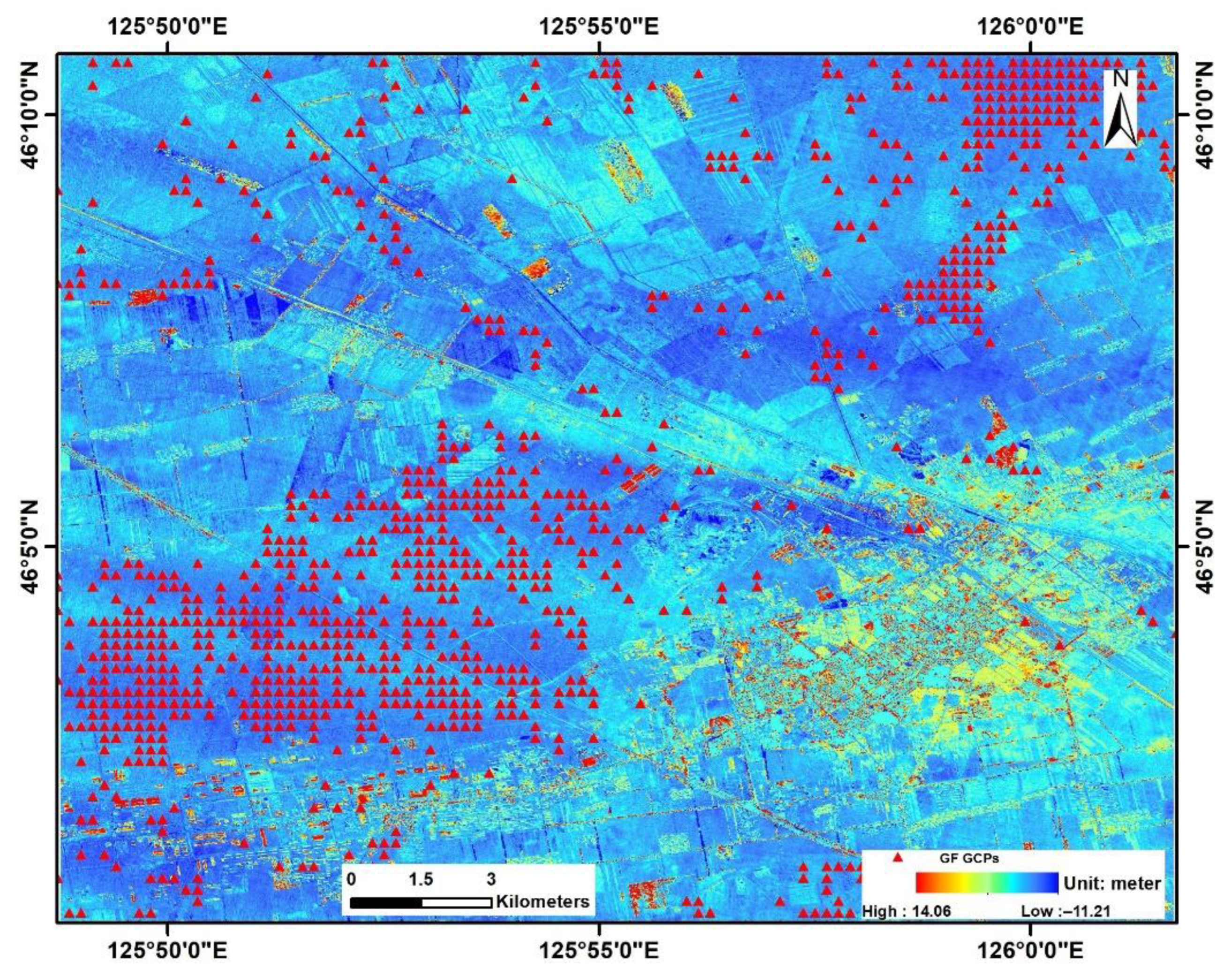
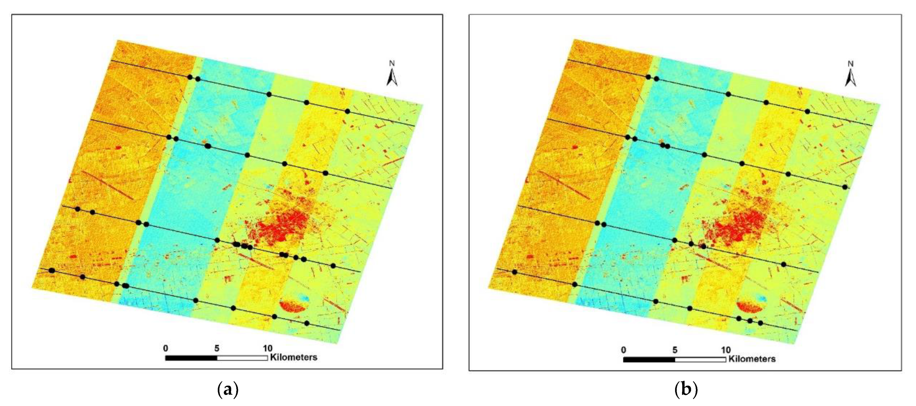
Data used in this paper are DSM derived from GF-7 stereo images and DSM derived from GFDM satellite images and the difference DSM between the two and the reference DSM. The image information used is shown in Table 1. The reference data are DSM obtained from 20 cm aerial imagery after manual editing, and the horizontal and vertical accuracies are both better than 0.4 m. Figure 1 shows the reference DSM used in this study. Meanwhile, a large number of ground control points are used to verify and analyze image geometric calibration and DSM accuracy. There are 1356 GCPs in the coverage area of GF-7 image and 4598 GCPs used in the coverage area of GFDM images in this paper. Figure 2 and Figure 3, respectively, show the difference DSM distributions between GFDM DSM and reference DSM and the difference DSM distributions between GF-7 DSM and reference DSM. The triangles in the figure are the distributions of GCPs used in our experiments.

Table 1.
Imagery data of GFDM and GF-7 used in this study.
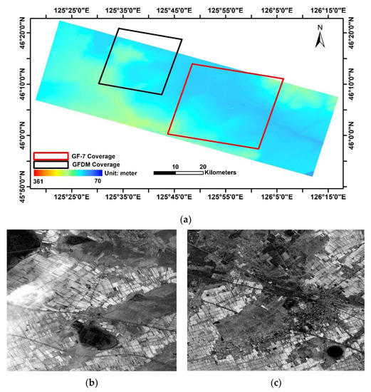
Figure 1.
(a) The reference Digital Surface Model (DSM) obtained from 20 cm aerial imagery in this study; (b) GFDM panchromatic imagery; (c) GF-7 panchromatic imagery.
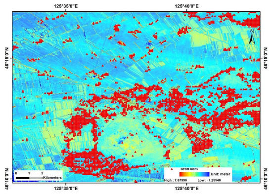
Figure 2.
The difference DSM distributions between GFDM DSM and reference DSM.

Figure 3.
The difference DSM distributions between GF-7 DSM and reference DSM.
It should be noted that it is better to use same reference (reference DSM and GCPs) to perform the comparation of the two DSMs. This means that there needs to be enough overlaps between the two comparing DSMs. However, the acquisition of GFDM stereoscopic imagery requires camera maneuvering, which leads limitation in obtaining stereoscopic coverage. So far, we only obtained one pair of suitable GFDM stereo images in the range of reference data. We selected a pair of GF-7 images with almost the same acquisition time as GFDM images, adjacent to GFDM coverage area with similar ground cover. Both of the GFDM and GF-7 images were obtained in November, when there are few other surface coverings, which are suitable for elevation accuracy evaluation. The reference DSM was generated with same datasets and processing flow, and GCPs observations were obtained at the same time with the same RTK equipment. Therefore, the accuracy consistency of reference data in each area can be guaranteed. Meanwhile, the inconsistency of surface changes can be largely eliminated, for the acquisition times of GFDM and GF-7 images are almost the same. Figure 1b,c shows the imagery taken from GFDM and GF-7 satellite in both study areas. Although the regions do not overlap, the two selected areas are adjacent, and the terrain in the study region is relatively flat with similar ground cover.
3. Method
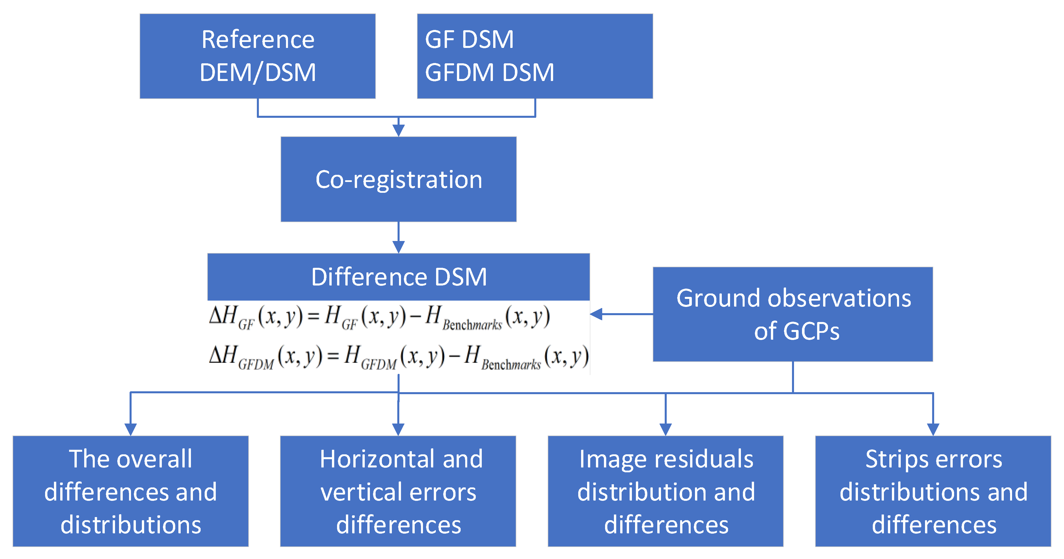
Comparison with high-precision reference DSM data is a common method for DSM accuracy evaluation. DSMs derived from GF-7 and GFDM are respectively compared with the high precision reference DSM using the calculated differences after co-registration with the reference DSM within the same coverage area. According to the DSM differences obtained, the accuracy and difference of GF-7 DSM and GFDM DSM are analyzed and evaluated. On the other hand, the differences between the two DSMs are extracted by GCPs measurements on the ground, and then, the object accuracy and image accuracy of GF-7 DSM and GFDM DSM are evaluated. Specifically, the evaluation includes the overall differential distribution of DSM and the reference DSM, horizontal displacement deviation and elevation deviation of DSM, the differences of residuals distribution in image space, and the strip error distributions based on differential DSM. The method flow is shown in Figure 4.

Figure 4.
Analysis of differences between GFDM DSM and GF-7 DSM using reference DSM and GCPs.
3.1. DSMs Generation and Co-Registration with the Reference DSM
Based on 3D terrain reconstruction from stereo images, a large number of GCPs are used to refine the rational function model of the images using block adjustment. The specific methods are described in the references and will not be repeated here [17]. In this paper, the image refinement model of affine transformation is adopted, and the error equation is
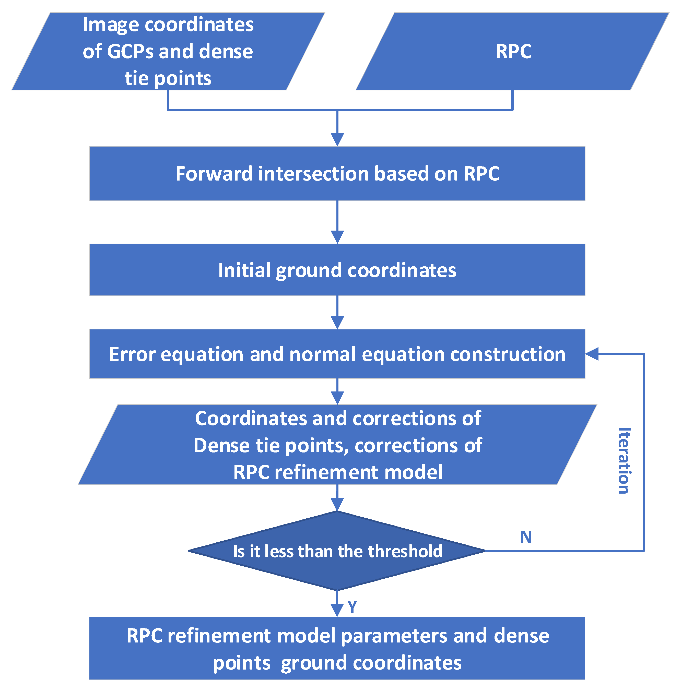
where, (X, Y) is the corresponding image measurement coordinates of GCPs; line and sample are the row and column coordinates of GCPs back-projected on the image space; and are coefficients of affine transformation. The flow of block adjustment using rational polynomial coefficient (RPC) [17,32] are shown in Figure 5. Then, DSM with a 2-m spatial resolution is generated through intensive matching of front and back images according to the refined RPC model. As the grid spatial resolution of reference DSM is one meter, which is higher than the 2-m spatial resolution of GFDM and GF7 DSMs, the bilinear interpolation method is used to resample the reference DSM to a 2-m grid to ensure the same resolution as the two DSMs. After that, the co-registration of the derived DSM and the reference DSM which is used as a benchmark is realized using least square correction, where the GCPs are used to establish the association between the derived DSM and the reference DSM.

Figure 5.
The flow of block adjustment using RPC.
3.2. Calculation of Differences between the Derived DSMs and the Benchmark
Assuming that and are two periods of DSMs after co-registration, and is the reference DSM as the benchmark,, are the 3D coordinates of a point in the same region corresponding to and , where and are the surface elevation values; then, the elevation difference at this point between the two DSMs is
Due to the inconsistency of data acquisition time, there is a certain time-varying difference or constant elevation difference between the two DSMs, and the difference with excessive elevation change needs to be eliminated. In this paper, outliers are removed according to the principle of 3 times standard deviation. If the difference value of one point was greater than 3 times standard deviation in the windows with n elevation differences, the point is an outlier and will be removed. That is
where, is the ith elevation difference value, and is the mean value of elevation difference.
3.3. Accuracy Check in Object and Image Space Using DSM Differences and GCPs
Since the different acquisition times of data, the surface has certain changes. In the comparison results between GF-7 DSM or GFDM DSM and the benchmark DSM, part of the differences is from the changes of surface itself over time, and this part leads to a larger overall error. However, the GCPs are almost set to observe at fixed points with surface unchanged, which have a more reliable reference accuracy. Therefore, ground observations from the GCPs are used as the high-precision reference data in the experimental coverage area. The coordinates and elevation values of GF-7 DSM or GFDM DSM are extracted according to the locations of GCPs, and the residuals of image space are calculated through back projection based on the extracted values. Then, according to the object observation deviations extracted from GCPs and the corresponding image residuals calculated, the accuracy of DSM in object and image space is analyzed, and the accuracy difference between GF-7 DSM and GFDM DSM is compared and evaluated.
Assuming that are the 3D coordinates of one GCP obtained by the ground measurements, are the GCP’s corresponding 3D coordinates of GF-7 DSM which are calculated by the forward intersection with the refined image transformation parameters, and are the GCP’s corresponding 3D coordinates from GFDM DSM with the same method, and the ground measurements are used as a benchmark, the elevation differences of both DSM are, respectively,
The horizontal differences are
Similarly, are the corresponding image coordinates of the GCP after the back projection to the image space. and are the corresponding image coordinates from GF-7 images and GFDM images. Then, the image residuals in X, Y, and Z three directions of GF-7 DSM are
the image residuals in X, Y, and Z three directions of GFDM DSM are
3.4. DSM Differences and Strip Errors
The attitude and position errors of satellite sensors as well as the different internal calibration methods lead to the inconsistency of DSM internal accuracy. As strips usually have certain systematic regularity or overall mutation with the normal, the strips will be more obvious after calculating the differences between the obtained DSM and the reference DSM. Therefore, the strip locations and fluctuation amplitudes can reflect the degree of inconsistency for DSM internal accuracy so as to evaluate the difference of internal accuracy between GF-7 DSM and GFDM DSM.
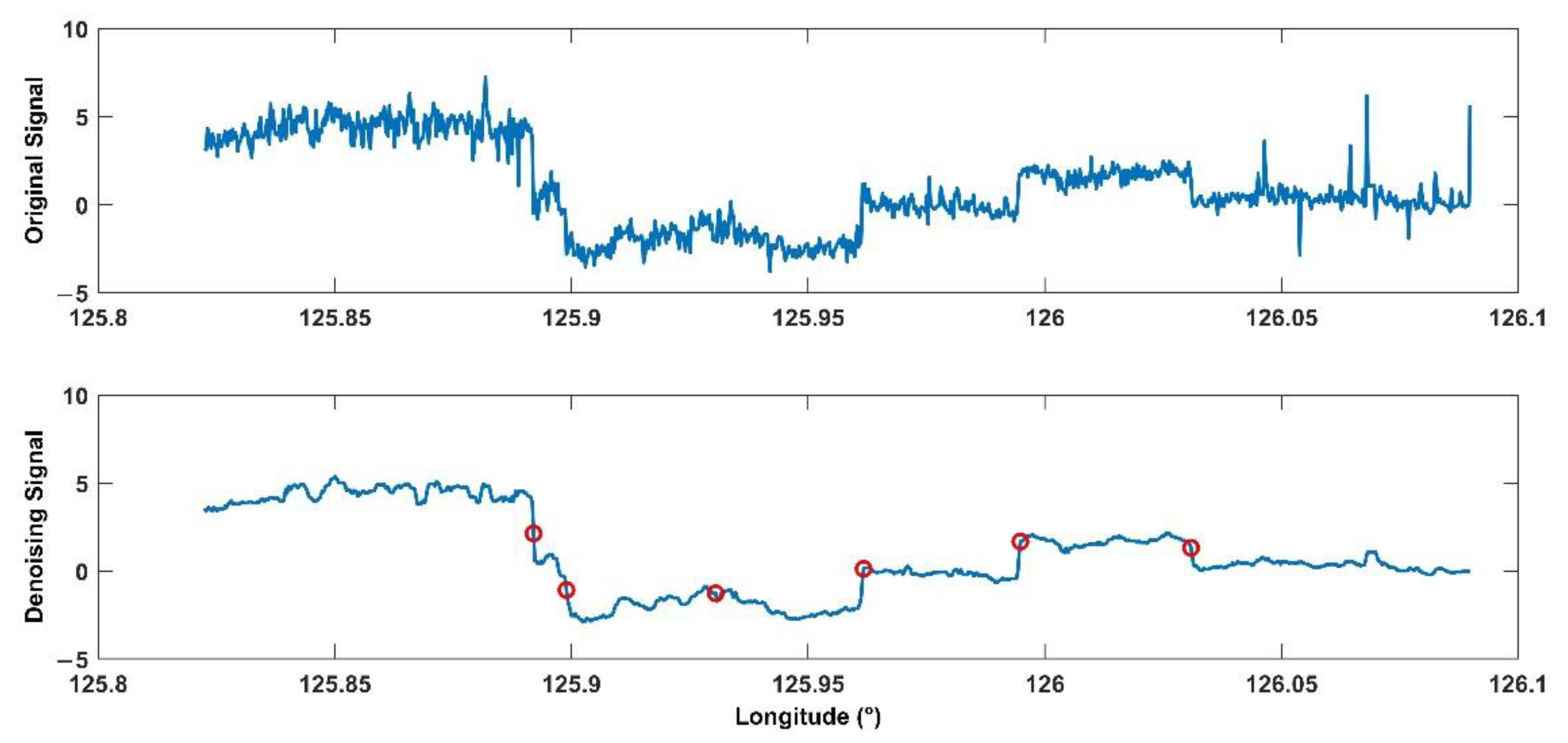
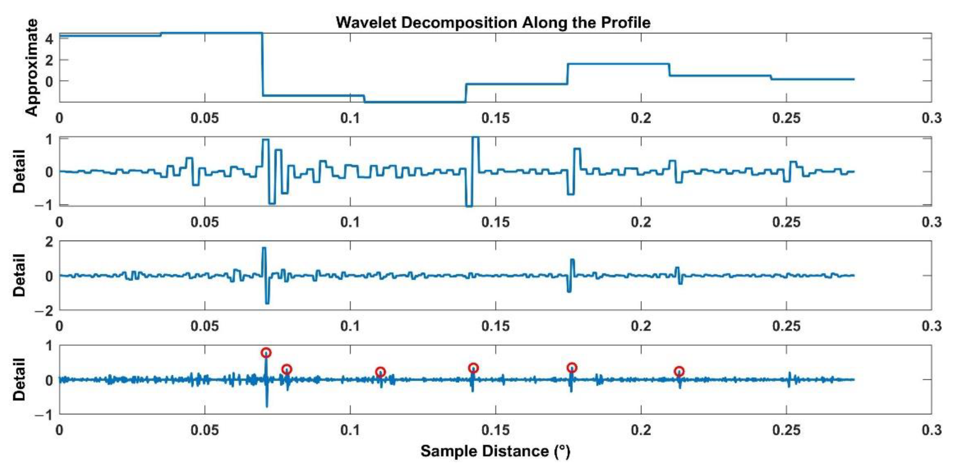
In this paper, the possible strips of GF-7 DSM and GFDM DSM are detected by the method of wavelet decomposition and wave peak-valley detection of profiles. The strips detected are compared and analyzed to obtain the accuracy differences between the two DSMs. Wavelet decomposition of profiles can detect the overall mutation position. The specific steps are as follows: Firstly, multiple profile lines are set up in the DSM region, and the values of elevation differences along the profile lines are extracted by the vectors. Secondly, the extracted elevation differences along the profiles are filtered, and then, decomposed by wavelet, and the approximate signals and the detailed signals of the profile lines after decomposition are obtained. Then, according to the peak mutation positions of detail signals and approximate signals, the overall mutation positions existing in the original profile lines are detected and obtained. Figure 6 shows the elevation differences extracted along one profile line before and after filtering. Figure 7 is the schematic diagram of approximate signals and detail signals after wavelet decomposition of the profile line, in which the red circles represent the detected mutation locations, namely the strips boundary locations.
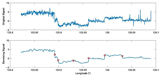
Figure 6.
Profiles before and after elevation differences filtering (red circles correspond to the mutation positions detected by wavelet analysis).
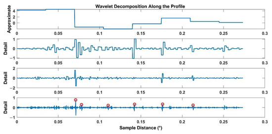
Figure 7.
Approximate signal and detail signal after wavelet decomposition along the elevation difference profile (red circles correspond to the mutation positions detected by wavelet analysis).
The method of wave peak–valley detection for profiles has a better effect for strips with certain regular changes and can estimate the fluctuation intervals and ranges of strips. Suppose that there are n elevation sampling points along the profile line, is the ith point on the profile, is the distance from the point to the starting point of the profile line, and is the elevation difference extracted from this point. According to the difference between each point and adjacent points along the line, a window with length len is taken to extract the maximum elevation difference point and minimum elevation difference point in the window respectively. To avoid generating too many extreme points, the distance interval threshold and elevation difference drop threshold between adjacent extreme points are set, the extreme points with interval less than and elevation difference drop less than are removed. The maximum and minimum points retained are the peak points and valley points of the profile line, respectively.
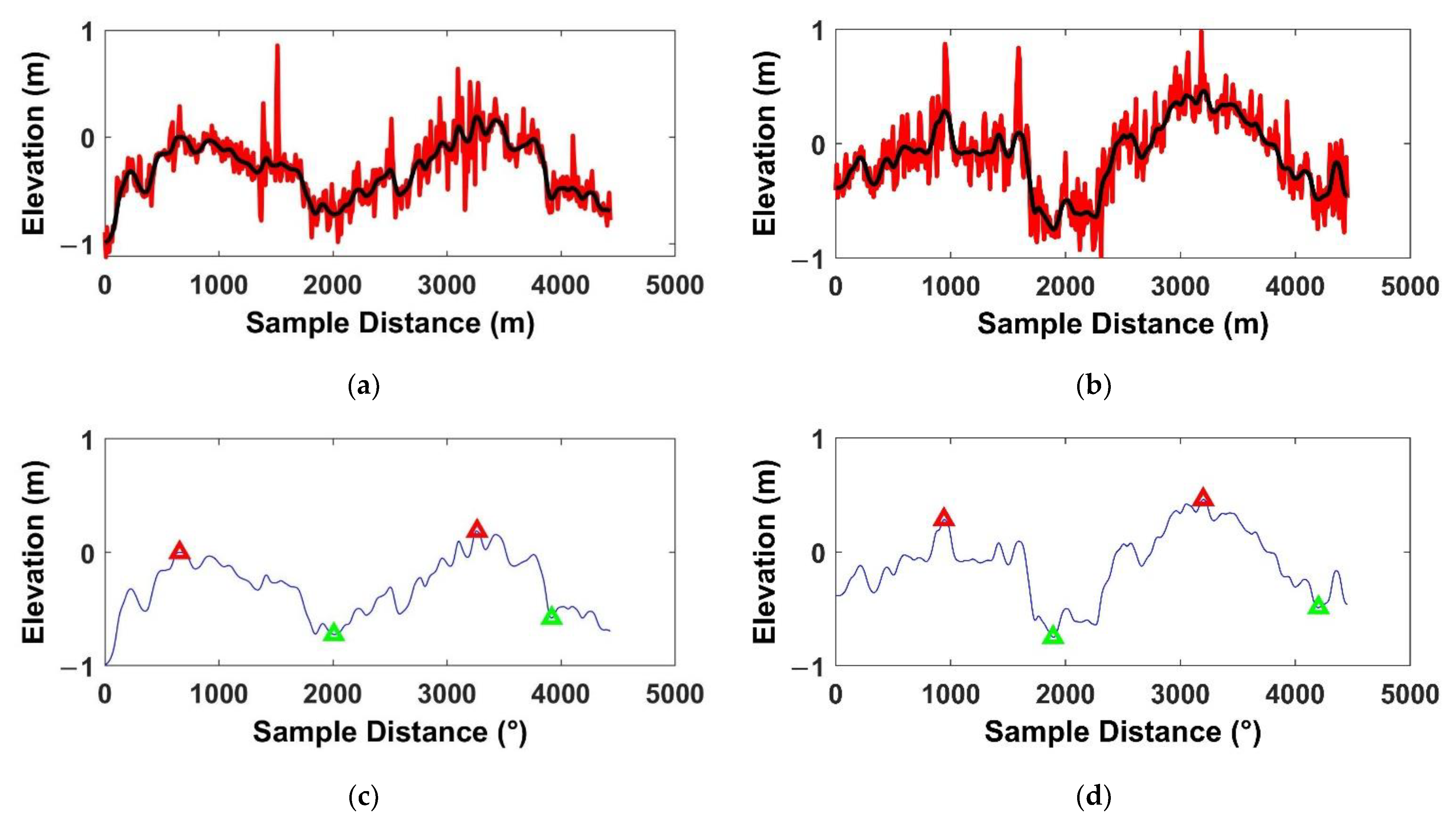
Let and be the reserved m peaks and k valleys, the average amplitude of peaks is , and the average amplitude of valleys is , then the elevation fluctuation range of the strip is . Figure 8 shows the positions of the wave peaks and valleys of the profile line detected by this method, and the interval distances of the strips fluctuations is calculated according to their positions
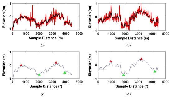
Figure 8.
The positions of wave peak–valley detection for profiles. (a,b) are examples of profiles before (red lines) and after (black lines) elevation differences filtering. (c,d) are the positions of peak (red triangles) and valley (green triangles) which indicate the mutation positions of strips.
Strip positions are flanked by areas with large differences which means the DSM internal accuracy is inconsistent. The interval and amplitude of strips fluctuations reflect the differences between the DSM and the benchmark DSM and also reflect the errors during the early DSM calibrations.
4. Results
This paper extracted and compared the differences between GF-7 DSM and GFDM DSM by using high-precision reference DSM and GCPs. The results include the overall differences between the two DSMs and the reference DSM, the differences of DSM horizontal displacement deviations and vertical errors, residuals differences in image space, coupling differences between vertical errors and image residuals, and differences of strip distributions.
4.1. The Overall Differences between GF-7 DSM and GFDM DSM with High-Precision Reference
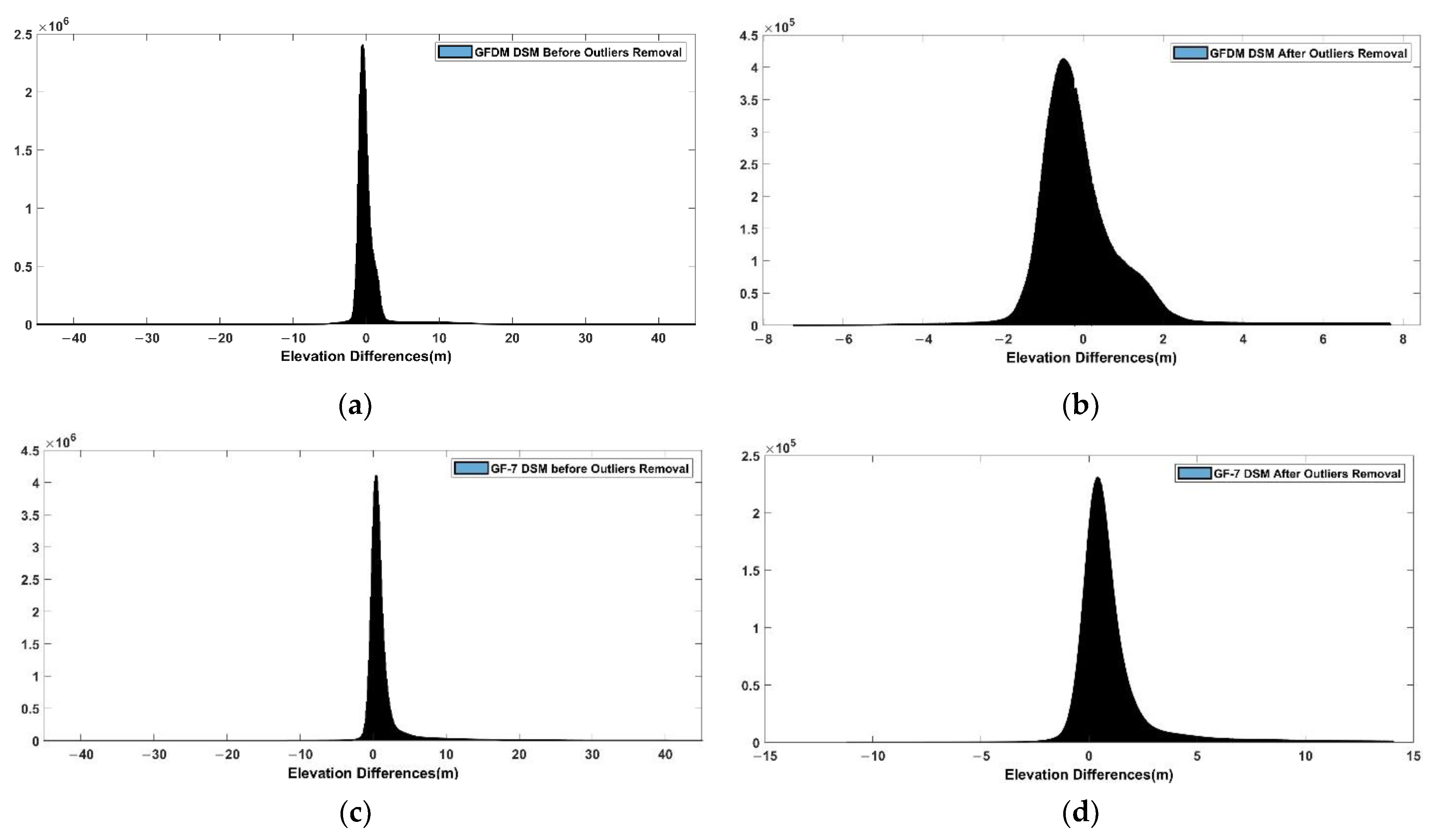
According to the calculation of differences in Section 3.2, GF-7 DSM and GFDM DSM are respectively evaluated with the corresponding high-precision reference DSM to obtain the overall differences between them and the reference DSM. Outliers with greater than 3 times standard deviation are removed. The removed outliers are about 2.66% in GFDM DSM and 1.69% in GF-7 DSM. Most of them are located in areas with obvious boundary characteristics, such as roads or houses. In this study, these values with large errors are not involved in the statistics for accuracy evaluation.
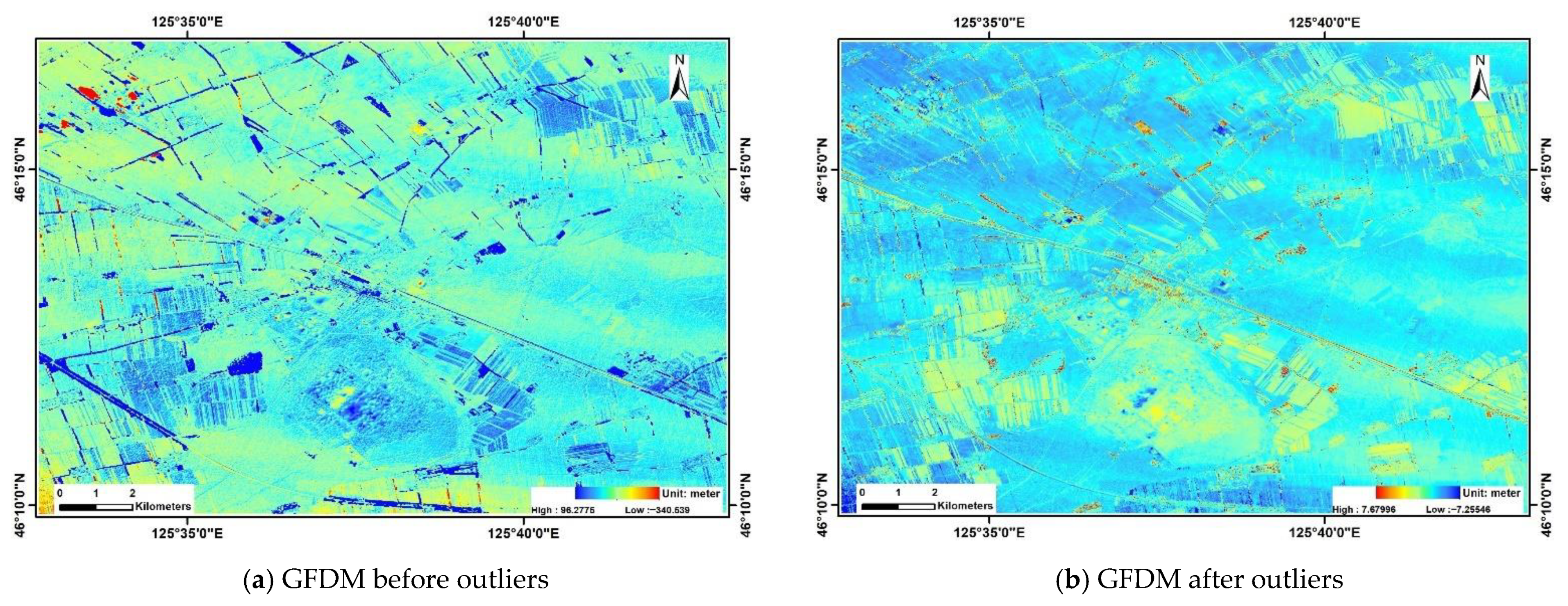
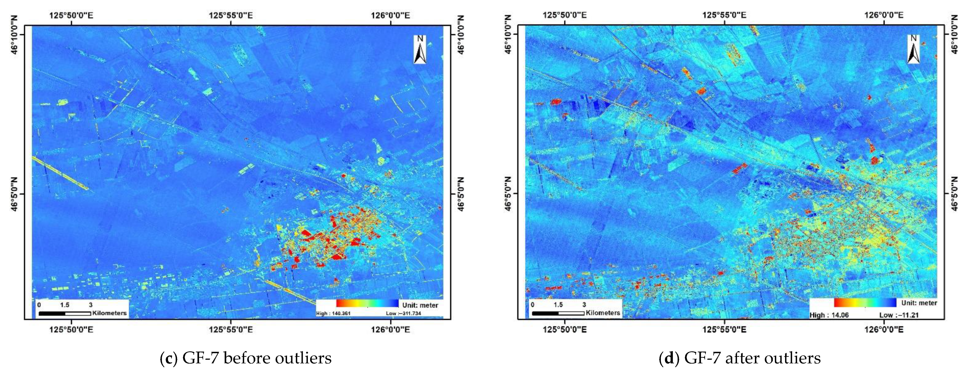
Figure 9 shows the spatial distributions of the overall differences between the two DSMs and the benchmark before and after outliers removed. Figure 10 shows the corresponding histograms of the two DSMs. Table 2 shows the statistical results of the overall differences before and after the exclusion of outliers. It can be seen from that, after the outliers are removed, that the average of elevation differences from GF-7 DSM is about 1 m, while the average from GFDM DSM is about −0.03 m, and the latter is closer to zero. In terms of RMSE of the overall differences, the RMSE of GF-7 DSM is about 1.90 m, and that of GFDM DSM is about 1.21 m. That means the overall differences between GF-7 DSM and the reference DSM are larger than that between GFDM-7 DSM and the reference DSM.
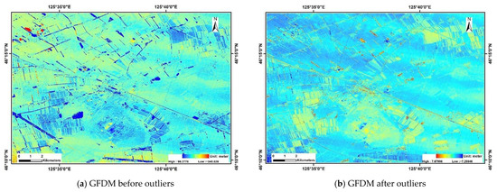
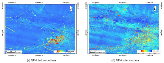
Figure 9.
GFDM and GF-7 difference DSMs before and after outliers were removed: (a) GFDM difference DSM before outliers were removed; (b) GFDM difference DSM after outliers were removed; (c) GF-7 difference DSM before outliers were removed; (d) GF-7 difference DSM after outliers were removed.
Figure 10.
Histograms of GFDM and GF-7 difference DSMs before and after outliers were removed: (a) histogram of GFDM difference DSM before outliers were removed; (b) histogram of GFDM difference DSM after outliers were removed; (c) histogram of GF-7 difference DSM before outliers were removed; (d) histogram of GF-7 difference DSM after outliers were removed.
Table 2.
Statistics of the overall differences between GFDM DSM and GF-7 DSM.
4.2. Differences of Horizontal Displacement Deviations and Vertical Errors
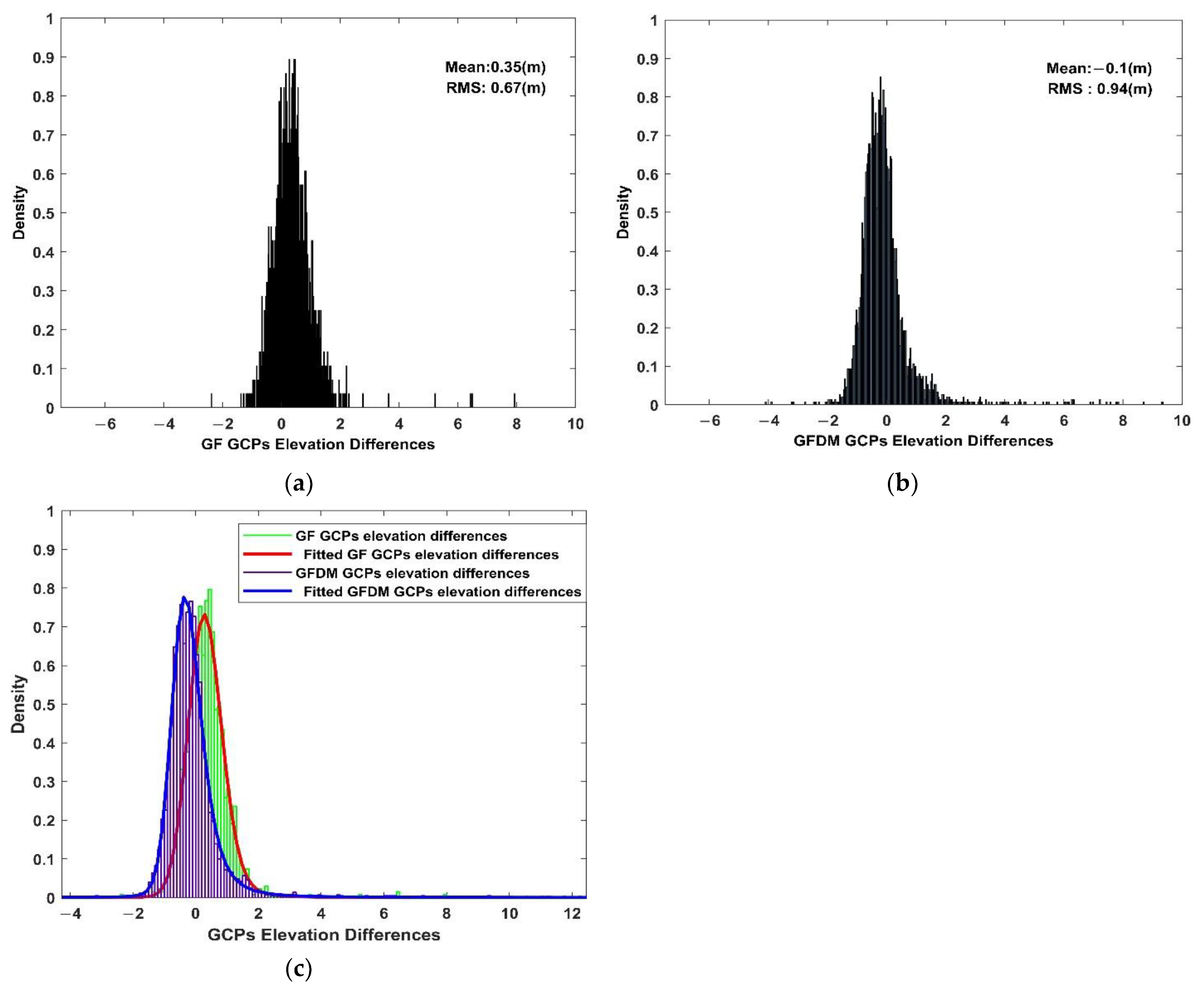
There are 1356 GCPs for GF-7 DSM and 4598 GCPs for GFDM DSM which are set up and used in the study area to evaluate the accuracy of DSM horizontal deviations and vertical errors. Table 3 is the comparative statistical results of horizontal and vertical accuracies obtained by using these GCPs for GF-7 DSM and GFDM DSM. The results show that their horizontal precisions are very close for the RMSE of both horizontal deviations, these being in the range of 0.51~0.53 m. The RMSE of vertical errors for GF-7 DSM is 0.67 m while it is 0.94 m for GFDM DSM, which is slightly larger than GF-7 DSM by 0.27 m. However, both of the RMSE of vertical errors are within 1 m. Figure 11 shows the vertical errors distributions of the two DSMs based on the extraction of local results (Figure 11a,b) and the histogram comparison results of vertical errors between the two DSMs (Figure 11c). The histograms show that the mean elevation error of GFDM is closer to zero, but the holistic concentration is slightly worse than that of GF-7 DSM.
Table 3.
Comparative statistics of horizontal and vertical accuracies of GFDM DSM and GF-7 DSM using GCPs.
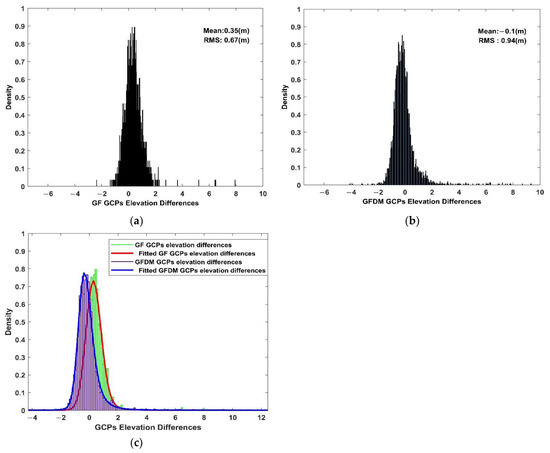
Figure 11.
Histograms of (a) GF-7 DSM differences; (b) GFDM DSM differences; and (c) GF-7 DSM differences and GFDM DSM differences comparison based on ground observations.
4.3. Residuals Differences in Image Space
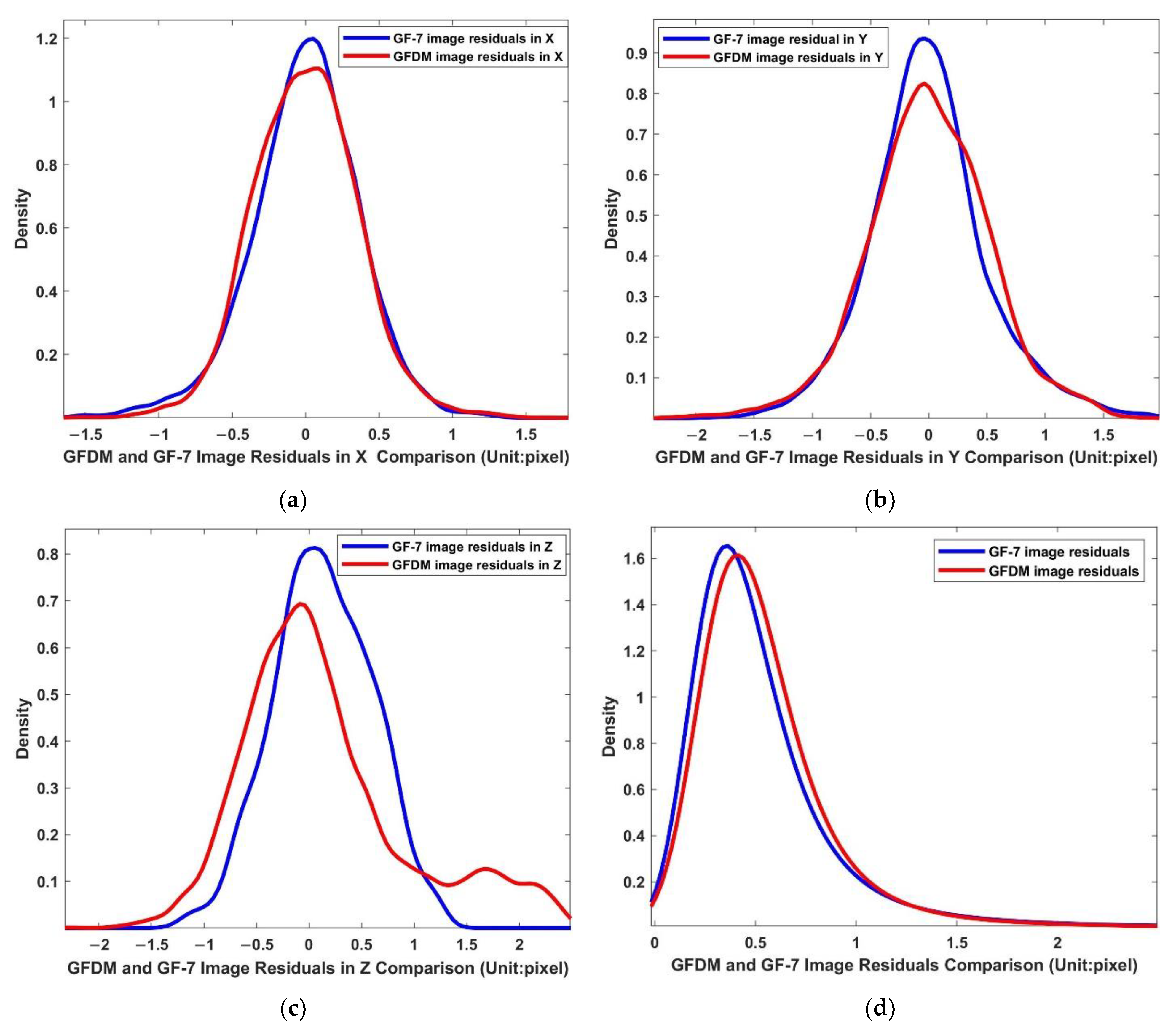
Figure 12 shows the distributions of image residuals for these GCPs used in GF-7 and GFDM DSM. Figure 12a–c shows the residuals in the X, Y and Z directions, respectively, and Figure 12d shows the distribution of the overall image residuals. The detailed statistical results are shown in Table 4. From the results, the accuracy of image space is similar to that of object space. The image residuals of GF-7 DSM are all within 0.5 pixels, and the effect of zero concentration is slightly better than that of GFDM DSM. The image residuals in the X and Y directions are very close for both GF-7 and GFDM DSM. However, their residuals in the Z direction differ greatly because the RMSE of residuals in the Z direction of GFDM DSM is 0.80 pixel, lower than that of GF-7 DSM, which the RMSE is 0.47 pixel.
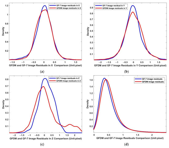
Figure 12.
Comparison of image residuals for GFDM DSM and GF-7 DSM based on GCPs: (a) image residuals in X; (b) image residuals in Y; (c) image residuals in Z; (d) all image residuals.
Table 4.
Image residuals statistics of GFDM DSM and GF-7 DSM based on GCPs.
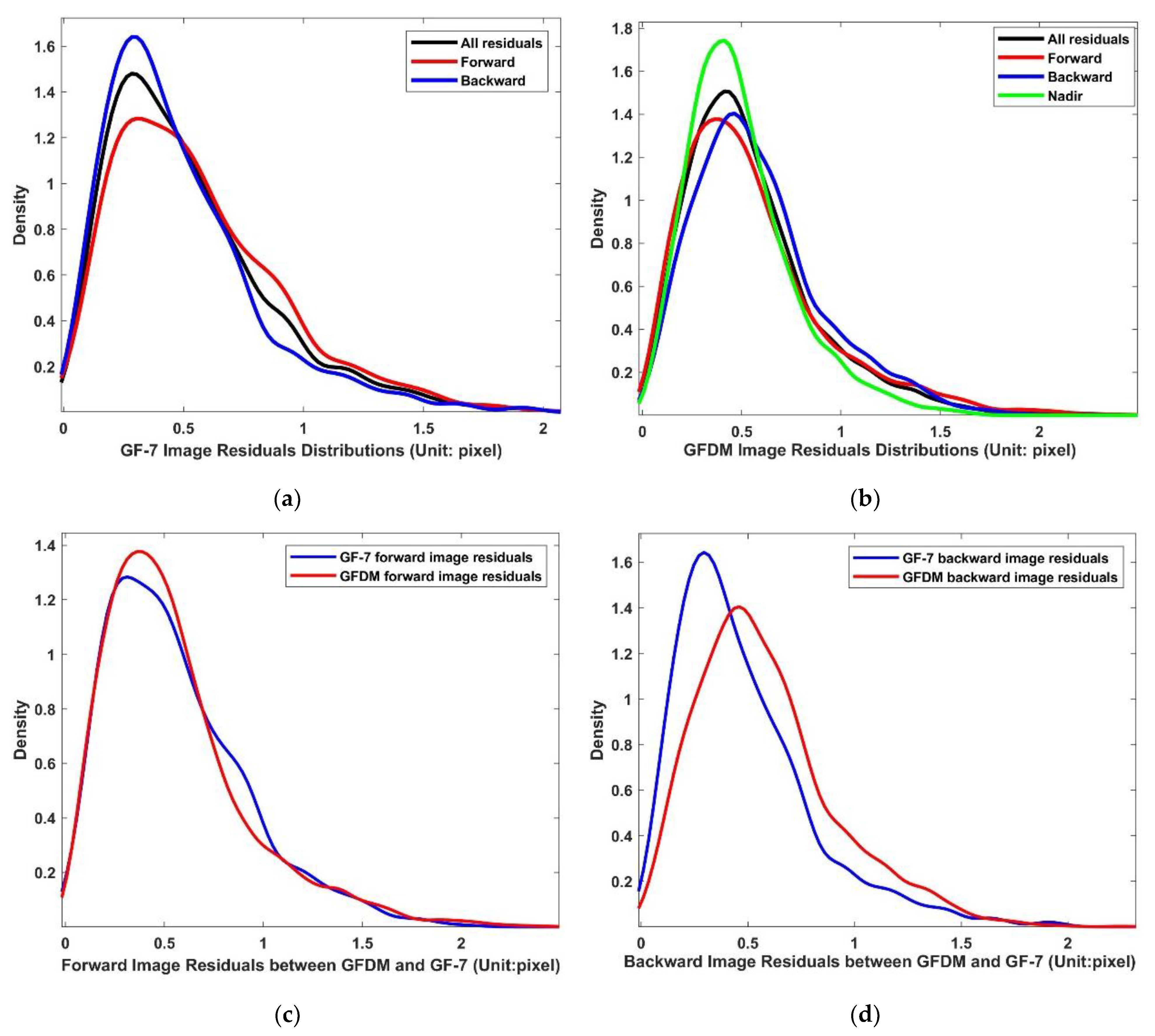
Since the images of GF-7 and GFDM satellites acquired are linear array images, the image residuals are also different under different viewing angles. Figure 13 shows the comparison of image residuals for GF-7 DSM and GFDM DSM, especially the differences from forward and backward images. Figure 13a shows the image residuals distribution of the forward-backward images of GF-7 DSM, and the residuals distribution of backward imagery is superior to that of forward imagery. Figure 13b shows the image residuals distribution of the forward-nadir-backward images of GFDM DSM. The residuals accuracy of the nadir image is better than both those of forward and backward images. In addition, consistent with GF-7 DSM, the residuals distribution of GFDM backward imagery is worse than that of forward imagery. Figure 13c,d, respectively, show the residual comparison of forward images and backward images for the two DSMs. According to the comparison results, the forward image residuals accuracy of GFDM DSM is slightly better than that of GF-7 DSM, while the backward image accuracy of GF-7 DSM is better than that of GFDM DSM. Considering the viewing angles of GFDM and GF-7 forward images, the observation Angle is −26 degrees, and the other is −25 degrees. Therefore, their forward accuracy is basically consistent. However, the viewing angles are +25 degrees and +5 degrees for GFDM and GF-7 backward images, respectively, this leads the differences in the backward image accuracy. On the whole, the residuals distribution in image space of GF-7 DSM is better than that of GFDM DSM.
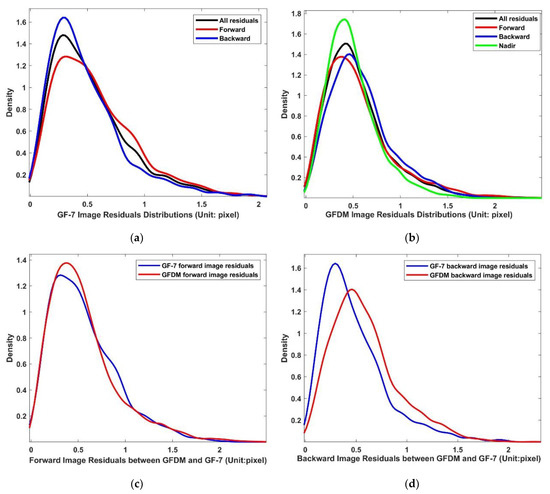
Figure 13.
Comparison of image residuals distributions with different views for GFDM DSM and GF-7 DSM: (a) distributions of GF-7 forward, backward, and all image residuals; (b) distributions of GFDM forward, backward, nadir, and all image residuals; (c) comparison of GFDM and GF-7 forward image residuals; (d) comparison of GFDM and GF-7 backward image residuals.
4.4. Coupling Differences between Image Residuals and Vertical Errors
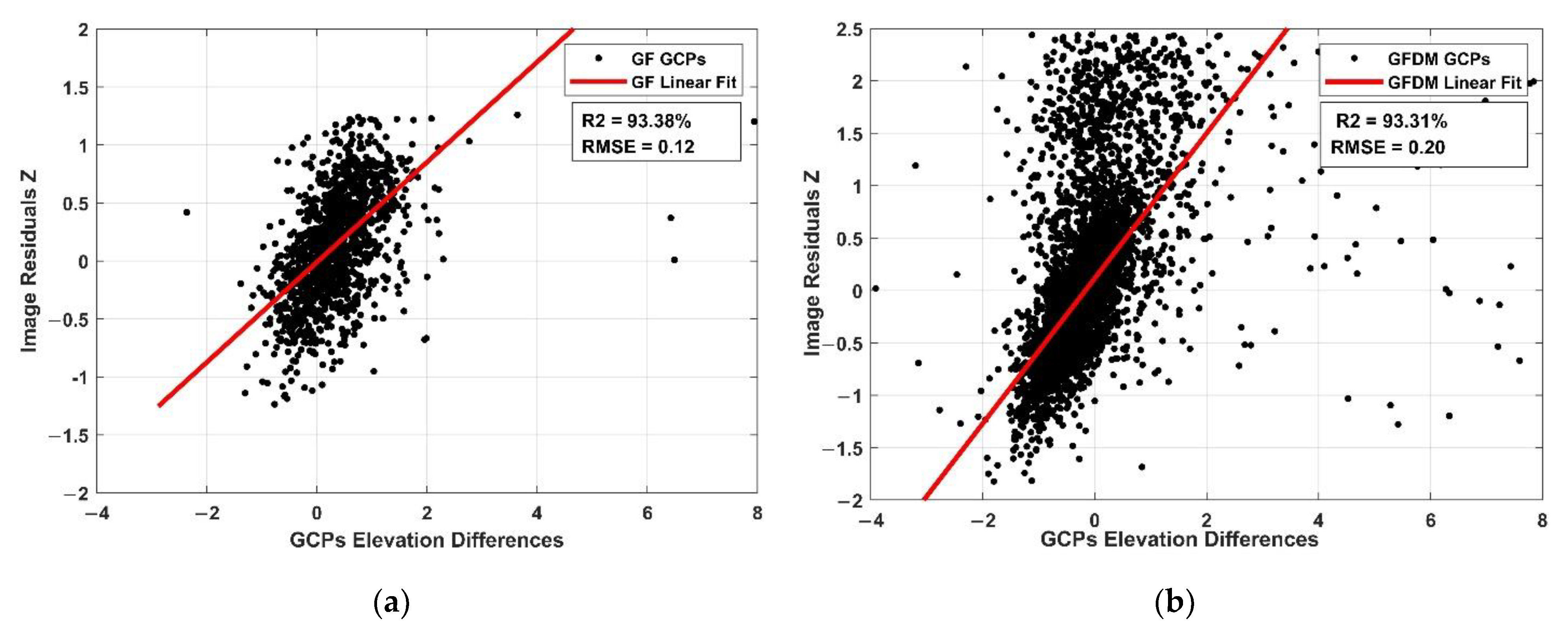
According to the results in Table 3 and Table 4, there is little difference for the image residuals in the X and Y directions between GF-7 DSM and GFDM DSM, and the distributions between the image residuals and the vertical errors are very similar. In order to further clarify the correlation between the image residuals and the vertical errors, Figure 14 and Figure 15, respectively, show the comparative relationship between image residuals and vertical errors in the three directions for GF-7 DSM and GFDM DSM. The figures show that most values in X and Y directions are near zero, and the relationship between image residuals and vertical errors is not obvious in X and Y directions for the two DSMs, which is similar to the result in Figure 12. However, being different from X and Y directions, the distributions of Z-direction residuals and vertical errors show some linear correlation. A linear regression model is used to fit the residuals in the Z-direction and vertical errors in GF-7 DSM, and the result is
where is the Z-direction residual, is the elevation error of GCP; the linear model fitting determination coefficient is about 0.9338, and the value of RMSE is about 0.12. The linear model of Z-direction residuals and vertical errors of GFDM DSM in the Z direction is
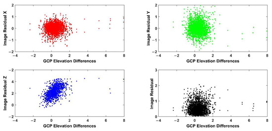
Figure 14.
The relationship between image residuals and object elevation differences for GF-7 DSM.
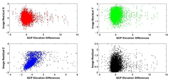
Figure 15.
The relationship between image residuals and object elevation differences for GFDM DSM.
The fitting determination coefficient is about 0.9331, and the value of RMSE is about 0.20. The fitting results are shown in Figure 16a,b. It can be seen from the results that there is a certain linear relationship between the image residuals in the Z direction and the vertical errors. The fitting RMSE in GF-7 DSM is smaller than that in GFDM DSM, indicating that the linear relationship between the image residuals and vertical errors in GF-7 DSM is more regular than that in GFDM DSM.
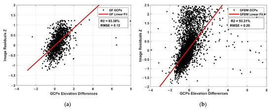
Figure 16.
Fitting results of residuals and elevation differences in the Z direction for (a) GF-7 DSM and (b) GFDM DSM.
4.5. The Strips Distributions and Differences between GF-7 DSM and GFDM DSM
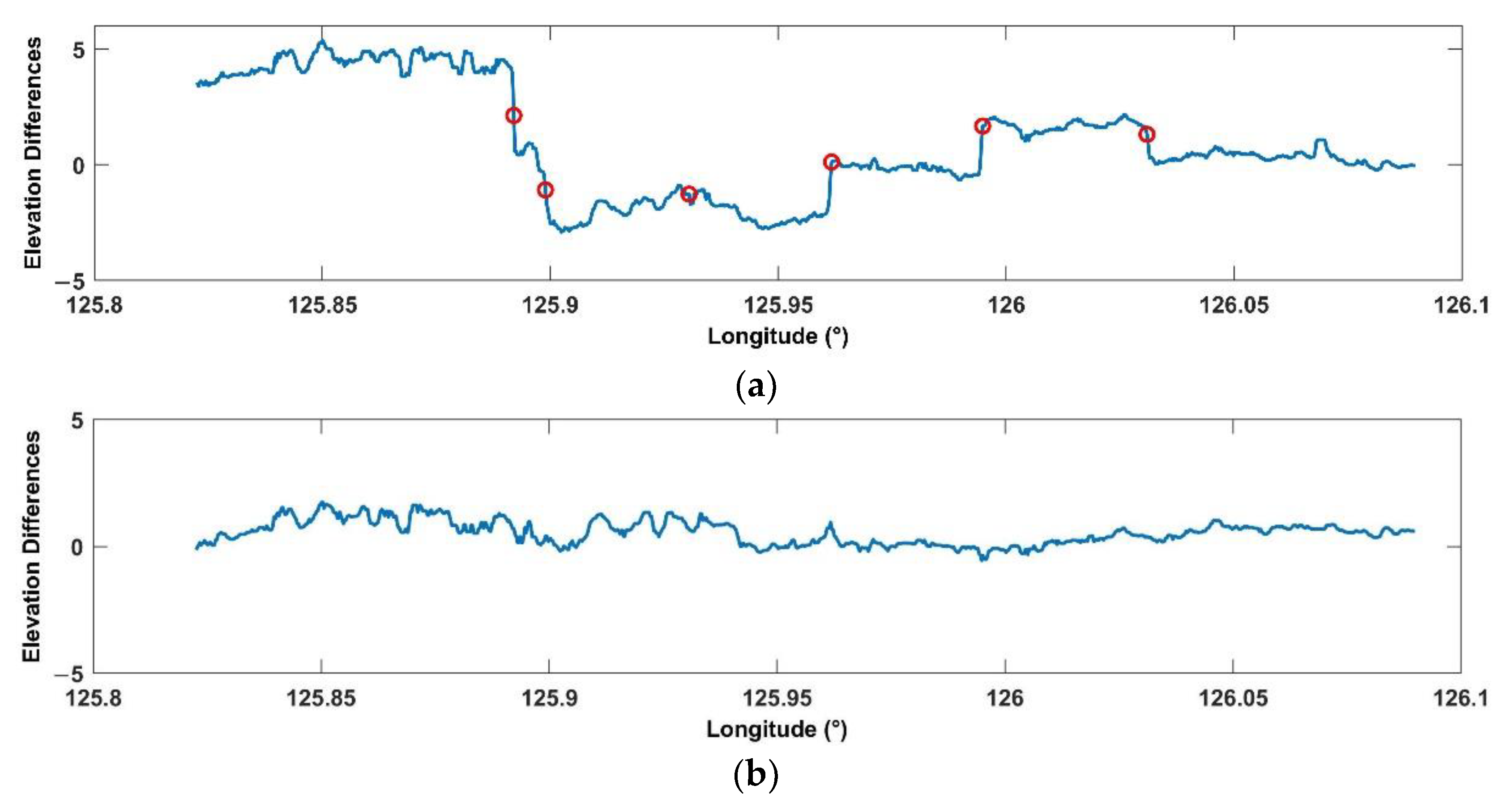
According to the strip’s detection described in Section 3.4, the strips which may possibly be in GF-7 DSM and GFDM DSM are detected and compared. From the display effects of the two DSMs in Figure 9, GF-7 DSM presents almost no obvious striping. In order to test the possible striping characteristics of GF-7 DSM, the DSM, before complete calibration, conduct strip detection. Figure 17 shows the strip position points of GF-7 DSM detected by 4 cross-track profiles (the black lines in Figure 17) using wavelet decomposition and wave peak-valley detection of profiles, respectively. From its distribution, all the mutation strips are detected, and these peak mutation points in cross-track are all at the edges of the strips, which is consistent with the DSM display visually. Because the strip changes irregularly, the strip positions detected by the wavelet decomposition method of profiles are more accurate than that by wave peak-valley detection. According to the detection results, at the edges of the strips, the elevation varies abruptly, and the amplitude of elevation differences is close to 5 m. The widths of strips are not uniform, and the average interval of the strips is about 0.0385°, about 4km. Figure 18 shows the elevation differences along the profile before and after calibration for GF-7 DSM. It indicates that the striping phenomenon of GF-7 DSM (Figure 17a) is almost eliminated after the calibration.
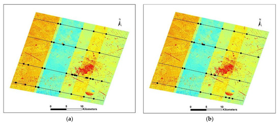
Figure 17.
Strip locations detected by (a) wavelet decomposition and (b) wave peak-valley detection (based on GF-7 DSM without calibration effectively).
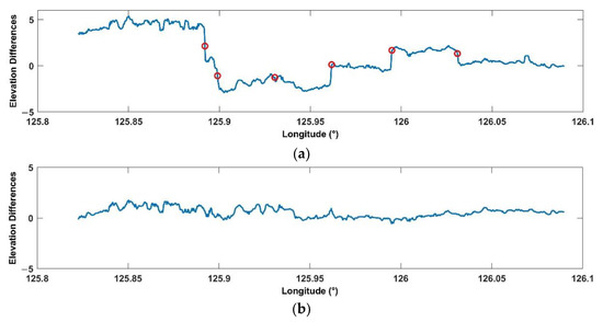
Figure 18.
The profiles of the northernmost line (a) without calibration effectively and (b) with effective calibration for GF-7 DSM. The red circles mark the locations of strips mutations.
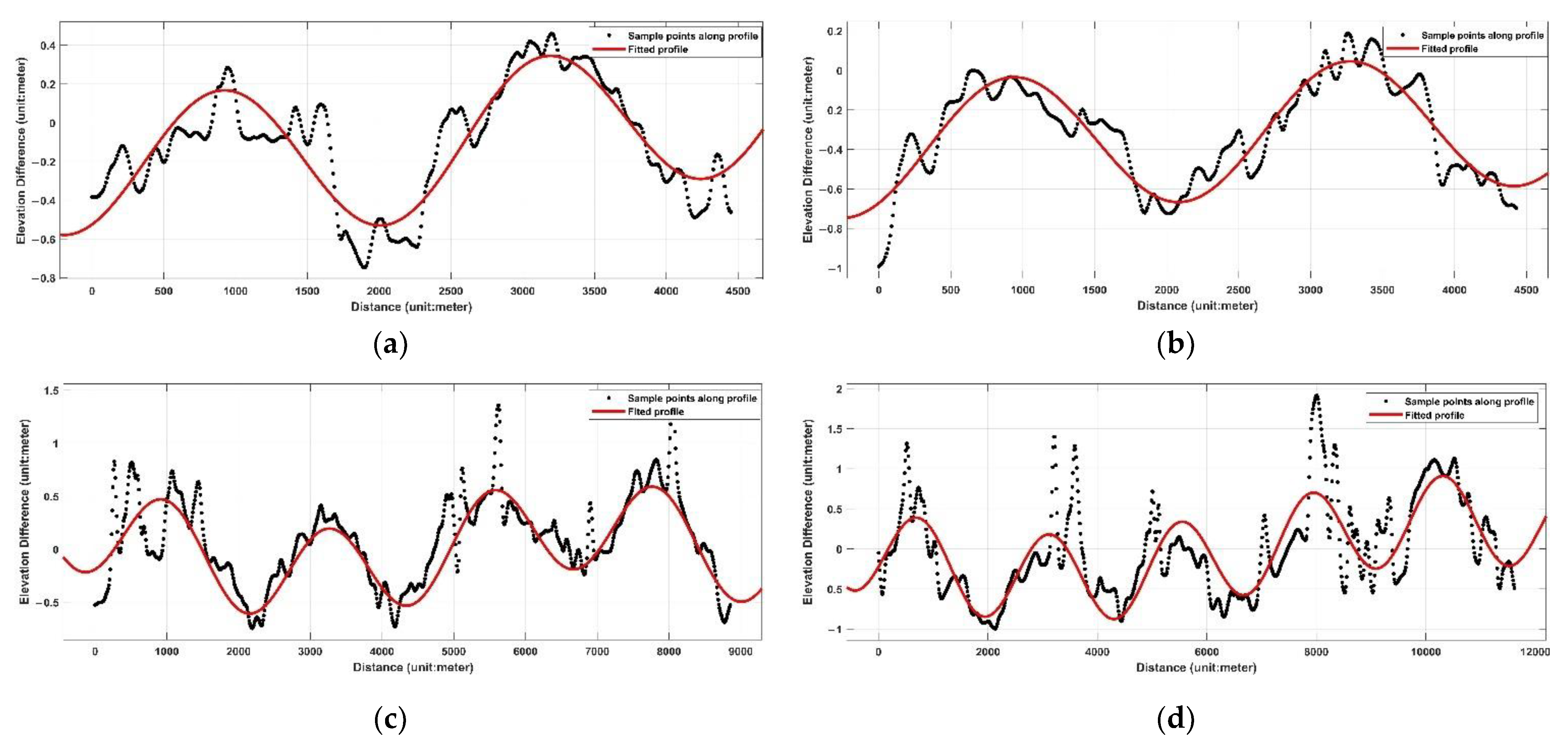
Compared with the irregularity of the strips or the disappearance after the calibration of GF-7 DSM, the strips in GFDM DSM are relatively regular (the pale-yellow diagonal strips in Figure 9), showing almost equally spaced strips. In this study, 9 profile lines (as shown in Figure 19) are used, and the elevation differences along profiles are extracted. Figure 20 shows the elevation difference profiles of 4 of them. It can be seen from the figures that the vertical errors along the profile fluctuate, but they show obvious regular sinusoidal wave fluctuation after smoothing as shown with the red curves in Figure 19. According to the statistics of peak and valley points fitted along the profiles, the strip fluctuation interval of GFDM DSM is about 2400 m, and the amplitude range is between 0.33 and 0.64 m
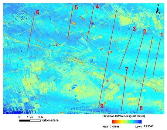
Figure 19.
The distributions of profiles for GFDM DSM.
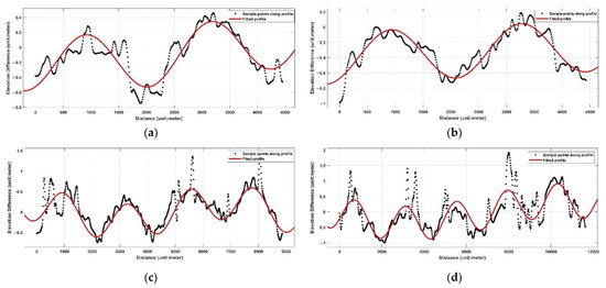
Figure 20.
Elevation differences along profiles: (a) Number 1; (b) Number 3; (c) Number 8; (d) Number 9 for GFDM DSM.
5. Discussion
5.1. The Factors of Accuracy Differences between the Two DSMs
GFDM DSM is very close to GF-7 DSM in accuracy. In terms of the overall difference between it and the reference DSM, the elevation accuracy of GF-7 DSM (1.90 m) is lower than that of DSM (1.21 m). However, the elevation accuracy evaluated by GCPs observation is opposite, and the elevation accuracy of GF-7 DSM (0.67 m) is better than that of GFDM DSM (0.94 m). On the whole, the accuracy deviation between the two DSMs is small. The factors of close accuracy differences between the two DSMs may include the following. The resolution of GFDM satellite imagery is slightly higher than that of GF-7 satellite, and the intersection angle of GFDM satellite is 52.454°, which is larger than that of GF-7 satellite (33.8°). At the same time, the base-height ratio of GFDM satellite (0.985) is slightly higher than that of GF-7 satellite (0.608). Theoretically, these advantage factors would make the DSM generated by GFDM satellite imagery more accurate than that of GF-7 DSM. However, due to the unstable attitudes of GFDM satellite, its accuracy relatively decreases, so there is not much difference between the overall accuracy of GF-7 DSM and that of GFDM DSM in the study area.
In addition to the above differences between the two DSMs when different reference data are used for evaluation, there are also great differences in the details of the two DSMs. According to the relationship between image residuals and vertical errors in Section 4.4, the fitting residuals of image residuals and vertical errors in GF-7 DSM are lower than those in GFDM DSM. To some extent, it also indicates that the errors caused by various factors in GF-7 DSM are more systematic and regular in the process of calibration, while the errors in GFDM DSM are more complex.
5.2. The Influence of GCPs on the Accuracy Differences
According to the distribution of GCPs shown in Figure 21, the locations of GCPs used in GF-7 DSM are more evenly distributed. On the other hand, although there are more ground points used in GFDM DSM, most points are located in the boundary or concentrated in a certain region in the middle of the test area. Moreover, according to the values of GCPs errors, the RMSE of these ground points is relatively higher than that of the whole GCPs. These factors also lead to that the elevation accuracy of GFDM DSM calculated by GCPs being lower than that of GF-7 DSM. However, the accuracy of GDM DSM is slightly better when the whole high-precision DSM within a large area is taken as the reference benchmark. Considering that there are certain surface changes in the study area, the evaluation based on GCPs is more convincing and reliable.
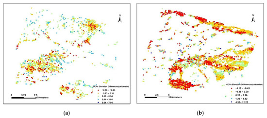
Figure 21.
Distribution and elevation differences of GCPs of (a) GF-7 DSM and (b) GFDM DSM in the study area.
5.3. The Influence of Data Processing on the Accuracy Differences
Bilinear interpolation is used to resample the reference DSM with 1-m grid to 2-m grid to ensure the same resolution as the two DSMs during the comparison. To clear the impact of interpolation on accuracy, elevation values in original reference DSM (1-m grid) and resampled DSM (2-m grid) are extracted using discrete GCPs points, respectively; then, both of the values are compared to the observations obtained by GCPs. Figure 22 shows the elevation differences between the resampled DSM and original DSM using 1356 extracted points. The average difference between the two is 0.00001 m, and RMSE is about 0.0019 m. That means the errors caused by interpolation can be negligible when compared with the accuracy of GFDM and GF-7 DSM.
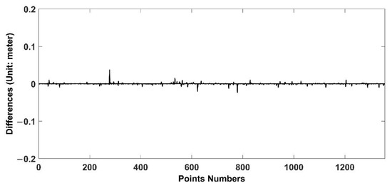
Figure 22.
The elevation differences between the resampled reference DSM and the original reference DSM.
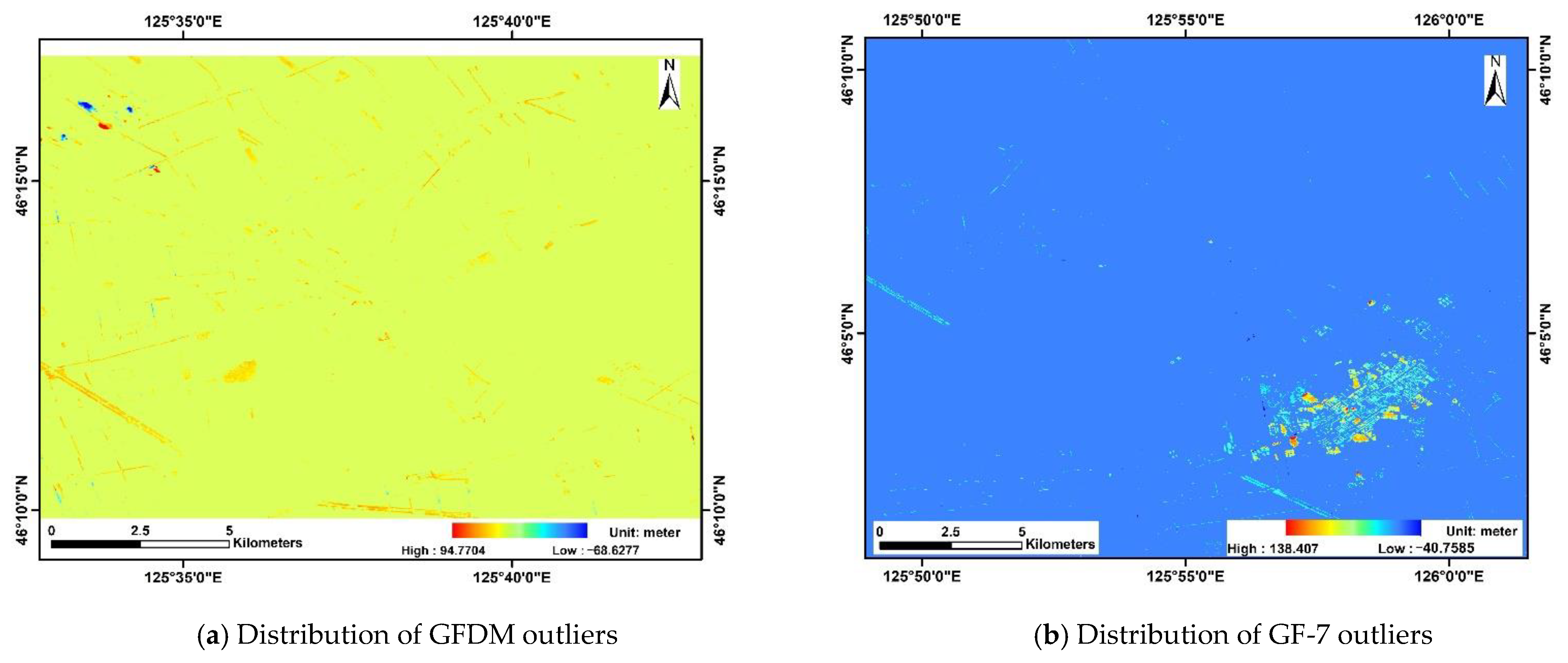
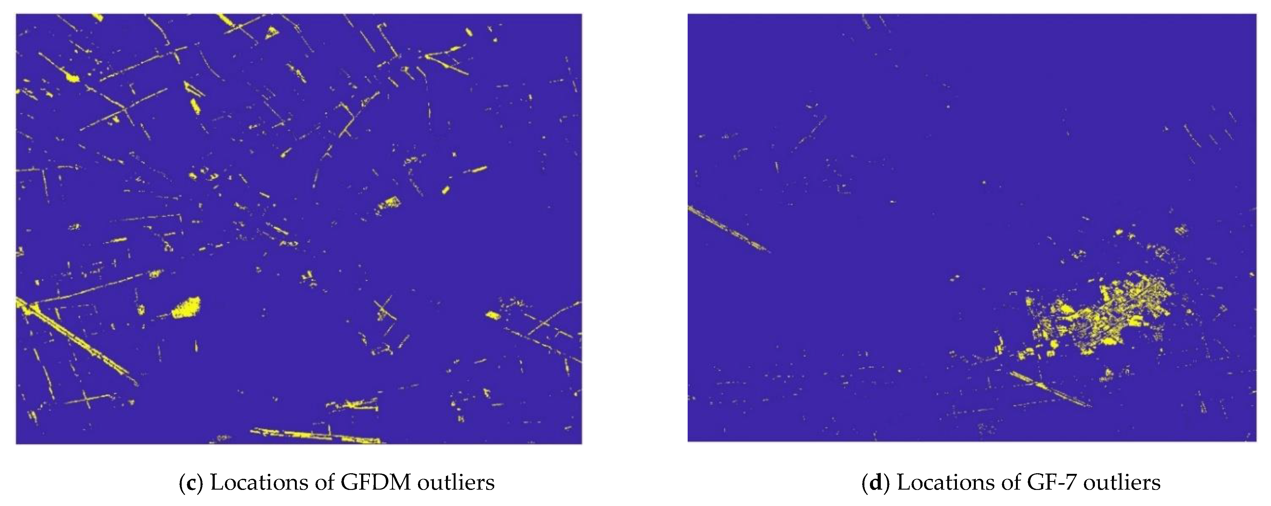
Outliers can be caused by a variety of factors, including surface changes, satellite positions and attitudes, and data processing methods. The instants of acquisition of the two DSMs in investigation, the reference DSM and the GCPs, are different, which would lead to some outlier causing by surface changes. This is also the main reason for removing outliers. In the comparison of the two DSMs, the reference DSM used is consistent for the same acquisition time and data process, and the same for GCPs. The acquisition times of GFDM and GF-7 images are almost the same, which can also ensure the consistent surface changes. Figure 23 shows the outliers distribution in GFDM difference DSM and GF-7 difference DSM. Figure 23c,d displays the locations of outliers more clearly after image binarization. Most of them are located in the areas with obvious boundary characteristics, such as roads or houses. Although the regions do not overlap completely, the inconsistency of surface changes can be largely eliminated according to the method described in Section 3.2. In this study, outliers are not involved in the accuracy evaluation. However, in subsequent studies, data with complete overlapping region and overlapping time may be better for the elimination of inconsistent surface changes.
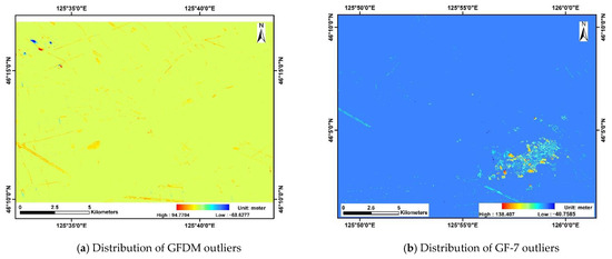
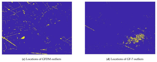
Figure 23.
Outliers in the two DSM: (a) outliers in GFDM difference DSM; (b) outliers in GF-7 difference DSM; (c) outliers locations in GFDM difference DSM; (d) outliers locations in GF-7 difference DSM.
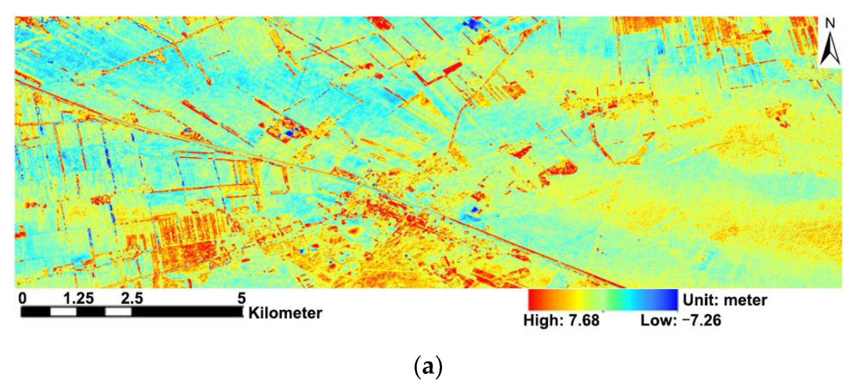
The discrepancy of imaging attitudes and positions and different calibrations will lead to different accuracies of DSMs. Inconsistent accuracy of calibration results in inconsistent errors distribution for DSM and also serious striping phenomenon. As shown in Figure 17, the strips in GF-7 DSM without effective calibration are very obvious, and the differences between strip and strip are large. However, there are abrupt changes at the strip edges; the internal accuracy in each strip is consistent, and the adjusted DSM with effective calibration has almost no strips. There are still striping phenomena in GFDM DSM after the calibration (Figure 19), which means that there are still certain errors in the DSM. This can also be seen from the small peak to the right of the main peak in the vertical errors histogram in Figure 10. Considering that the fluctuation amplitude of strips in GFDM DSM is small, and the strips fluctuate regularly, frequency filtering can be adopted to remove the strips. Figure 24 shows the removal effect after frequency blocking filtering. This also means that the calibration in the front-end can still be improved for DSM, or if it is insufficient, the later strips filtering can also improve the DSM effect.

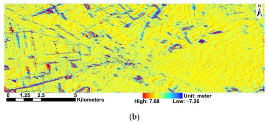
Figure 24.
GFDM DSM (a) before and (b) after strips elimination.
6. Conclusions
Using high-precision DSM and GCPs’ observations as the reference, DSM global accuracy, horizontal and elevation accuracy, the relationship of image residuals and vertical errors, and DSM strips are compared and evaluated between the two DSMs derived from GF-7 satellite imagery and GFDM satellite imagery, in this paper. The overall accuracy of the two is close; especially, the difference in horizontal accuracy is small. The elevation accuracy is slightly different when adopting a different reference terrain. If regional high-precision DSM is taken as the reference terrain, GFDM DSM has a slight advantage in elevation accuracy, but there are regular fluctuation strips with small amplitudes. Under the condition of scattered GCPs being the reference, GF-7 DSM has better elevation accuracy than GFDM DSM, but the elevation errors of both are within 1 m. The image residuals in three directions of GF-7 DSM are all within 0.5 pixels, while the image residuals in Z-direction of GFDM DSM are the relative maximum, reaching 0.8 pixels. DSM accuracy is closely linked to sensors, attitudes, position, different calibrations, and the ground environment. This paper only makes the analysis and assessment for GFDM DSM and GF-7 DSM in one study area. In the future work, different calibration methods and more study area will be considered and validated for the accuracy of GFDM products.
Author Contributions
X.Z., B.L., and W.H. developed the main idea of this study and performed the data processing and analysis. X.T. and G.Z. gave support to the DEM generation and accuracy analysis and the discussion of the results. The detailed information is as follows: data curation, B.L. and W.H.; formal analysis, G.Z., B.L., and W.H.; methodology, X.Z., B.L., and W.H.; project administration, X.Z. and X.T.; supervision, G.Z. All authors have read and agreed to the published version of the manuscript.
Funding
This research was supported by the National Natural Science Foundation of China (Grant No. 41601500), partly by the National Key Research and Development Program of China (NO. 2018YFB0504903), the High Resolution Remote Sensing, Surveying and Mapping Application Demon-stration System (Phase II) (NO. 42-Y30B04-9001-19/21) and the Major Project of High Resolution Earth Observation System (No. GFZX0404130302). We thank the editorial help as well as academic suggestions from the anonymous reviewers.
Informed Consent Statement
Informed consent was obtained from all subjects involved in the study.
Data Availability Statement
GFDM imagery and GF-7 imagery acquired in November 2020 can be inquired through the website for China Resource Satellite Application Center (http://sasclouds.com/english/home, accessed on 16 November 2021). Illustrations in this paper were subject to no copyright restrictions.
Conflicts of Interest
The authors declare no conflict of interest.
References
- Mudd, S.M. Topographic Data from Satellites; Developments in Earth Surface Processes; Elsevier: Amsterdam, The Netherlands, 2020; Volume 23, pp. 91–128. [Google Scholar] [CrossRef]
- Li, D. China’s first civilian three-line-array stereo mapping satellite: ZY-3. Acta Geodaet. Cartograph. Sinica 2012, 41, 317–322. [Google Scholar]
- Gao, X.; Liu, Y.; Li, T.; Wu, D. High Precision DEM Generation Algorithm Based on InSAR Multi-Look Iteration. Remote Sens. 2017, 9, 741. [Google Scholar] [CrossRef] [Green Version]
- Vassilaki, D.I.; Stamos, A.A. TanDEM-X DEM: Comparative performance review employing LIDAR data and DSMs. ISPRS J. Photogramm. Remote Sens. 2020, 160, 33–50. [Google Scholar] [CrossRef]
- Li, Z.; Zhu, Q. Digital Elevation Model; Wuhan University Press: Wuhan, China, 2003. [Google Scholar]
- Tang, G. Digital Terrain Analysis on Loess Plateau of China; Science Press: Beijing, China, 2015. [Google Scholar]
- Rizzoli, P.; Bräutigam, B.; Kraus, T.; Martone, M.; Krieger, G. Relative height error analysis of TanDEM-X elevation data. ISPRS J. Photogramm. Remote Sens. 2012, 73, 30–38. [Google Scholar] [CrossRef] [Green Version]
- Boulton, S.J.; Martin, S. Which DEM Is Best for Analyzing Fluvial Landscape Development in Mountainous Terrains? Geomorphology 2018, 310, 168–187. [Google Scholar] [CrossRef]
- Wang, R.; Zhang, S.; Pu, L.; Yang, J.; Yang, C.; Chen, J.; Guan, C.; Wang, Q.; Chen, D.; Fu, B.; et al. Gully Erosion Mapping and Monitoring at Multiple Scales Based on Multi-Source Remote Sensing Data of the Sancha River Catchment, Northeast China. Int. J. Geo Inf. 2016, 5, 200. [Google Scholar] [CrossRef] [Green Version]
- Frey, H.; Paul, F. International Journal of Applied Earth Observation and Geoinformation On the suitability of the SRTM DEM and ASTER GDEM for the compilation of topographic parameters in glacier inventories. Int. J. Appl. Earth Obs. Geoinf. 2012, 18, 480–490. [Google Scholar] [CrossRef]
- Feng, Z.; Shi, D.; Chen, W.; Luo, A. The progress of French remote sensing satellite—From SPOT toward Pleiades. Remote Inf. 2007, 4, 87–92. [Google Scholar]
- Li, D.; Wang, M. A review of high resolution optical satellite surveying and mapping technology. Spacecr. Recov. Remote Sens. 2020, 41, 1–11. [Google Scholar]
- Gong, J. Progress in Data Processing and Analysis of Earth Observation; Wuhan University Press: Wuhan, China, 2007. [Google Scholar]
- Cao, H.; Liu, F.; Zhao, C.; Dai, J. The study of high resolution stereo mapping satellite. Nat. Remote Sens. Bull. 2021, 25, 1400–1410. [Google Scholar]
- Tang, X.; Xie, J.; Zhang, G. Development and status of mapping satellite technology. Spacecr. Recov. Remote Sens. 2012, 33, 17–24. [Google Scholar]
- Tang, X.; Zhang, G.; Zhu, X.; Pan, H.; Jiang, Y.; Zhou, P.; Wang, X.; Guo, L. Triple linear-array imaging geometry model of Ziyuan-3 surveying satellite and its validation. Acta Geod. Cartograph. Sin. 2012, 41, 191–198. [Google Scholar]
- Liu, B.; Sun, X.; Di, K.; Liu, Z. Accuracy analysis and validation of ZY-3′S sensor corrected products. Remote Sens. Land Res. 2012, 24, 36–40. [Google Scholar]
- Zhang, G.; Wang, T.; Li, D.; Tang, X.; Jiang, Y.; Pan, H.; Zhu, X. Block adjustment for ZY-3 satellite standard imagery based on strip constraint. Acta Geod. Cartograph. Sin. 2014, 43, 1158–1164. [Google Scholar]
- Li, G.; Tang, X.; Chen, J.; Yao, J.; Liu, Z.; Gao, X.; Zuo, Z.; Zhou, X. Processing and preliminary accuracy validation of GF-7 satellite laser altimetry data. Acta Geod. Cartograph. Sin. 2021, 50, 1–11. [Google Scholar] [CrossRef]
- Fan, L.; Wang, Y.; Yang, W.; Yu, L.; Zhang, G. GFDM-1 satellite system design and technical characteristics. Spacecr. Eng. 2021, 30, 10–19. [Google Scholar]
- Zhou, Q.; Liu, X. Digital Terrain Analysis; Science Press: Beijing, China, 2006. [Google Scholar]
- Yermolaev, O.; Usmanov, B.; Gafurov, A.; Poesen, J.; Vedeneeva, E.; Lisetskii, F.; Nicu, I.C. Assessment of Shoreline Transformation Rates and Landslide Monitoring on the Bank of Kuibyshev Reservoir (Russia) Using Multi-Source Data. Remote Sens. 2021, 13, 4214. [Google Scholar] [CrossRef]
- Bergstedt, H.; Jones, B.M.; Hinkel, K.; Farquharson, L.; Gaglioti, B.V.; Parsekian, A.D.; Kanevskiy, M.; Ohara, N.; Breen, A.L.; Rangel, R.C.; et al. Remote Sensing-Based Statistical Approach for Defining Drained Lake Basins in a Continuous Permafrost Region, North Slope of Alaska. Remote Sens. 2021, 13, 2539. [Google Scholar] [CrossRef]
- Ali, S.; Liu, D.; Fu, Q.; Cheema, M.J.M.; Pham, Q.B.; Rahaman, M.M.; Dang, T.D.; Anh, D.T. Improving the Resolution of GRACE Data for Spatio-Temporal Groundwater Storage Assessment. Remote Sens. 2021, 13, 3513. [Google Scholar] [CrossRef]
- Panagiotakis, E.; Chrysoulakis, N.; Charalampopoulou, V.; Poursanidis, D. Validation of Pleiades Tri-Stereo DSM in Urban Areas. Int. J. Geo Inf. 2018, 7, 118. [Google Scholar] [CrossRef] [Green Version]
- Li, P.; Shi, C.; Li, Z.; Muller, J.P.; Drummond, J.; Li, X.; Li, T.; Li, Y.; Liu, J. Evaluation of ASTER GDEM using GPS benchmarks and SRTM in China. Int. J. Remote Sens. 2013, 34, 1744–1771. [Google Scholar] [CrossRef]
- Courty, L.G.; Soriano-Monzalvo, J.C.; Pedrozo-Acua, A. Evaluation of open-access global digital elevation models (AW3D30, SRTM and ASTER) for flood modelling purposes. J. Flood Risk Manage. 2019, 12, e12550. [Google Scholar] [CrossRef] [Green Version]
- Liu, Z.; Zhu, J.; Fu, H.; Zhou, C.; Zuo, T. Evaluation of the Vertical Accuracy of Open Global DEMs over Steep Terrain Regions Using ICESat Data: A Case Study over Hunan Province, China. Sensors 2020, 20, 4865. [Google Scholar] [CrossRef] [PubMed]
- Ibrahim, M.; Al, A.; Barbara, M.; Pawan, K. An evaluation of available digital elevation models (DEMs) for geomorphological feature analysis. Environ. Earth Sci. 2020, 79, 1–11. [Google Scholar] [CrossRef]
- Grohmann, C.H. Evaluation of TanDEM-X DEMs on selected Brazilian sites: Comparison with SRTM, ASTER GDEM and ALOS AW3D30. Remote Sens Environ. 2018, 212, 121–133. [Google Scholar] [CrossRef] [Green Version]
- Novak, A.; Oštir, K. Towards Better Visualisation of Alpine Quaternary Landform Features on High-Resolution Digital Elevation Models. Remote Sens. 2021, 13, 4211. [Google Scholar] [CrossRef]
- Grodecki, J.; Dial, G. Block adjustment of high-resolution satellite images described by Rational Polynomials. Photogramm Eng Remote Sens. 2003, 69, 59–68. [Google Scholar] [CrossRef]


Publisher’s Note: MDPI stays neutral with regard to jurisdictional claims in published maps and institutional affiliations. |
© 2021 by the authors. Licensee MDPI, Basel, Switzerland. This article is an open access article distributed under the terms and conditions of the Creative Commons Attribution (CC BY) license (https://creativecommons.org/licenses/by/4.0/).