Land Cover Dynamics on the Lower Ganges–Brahmaputra Delta: Agriculture–Aquaculture Transitions, 1972–2017

Abstract

Aquaculture in tropical and subtropical developing countries has expanded in recent years. This practice is controversial due to its potential for serious economic, food security, and environmental impacts—especially for intensive operations in and near mangrove ecosystems, where many shrimp species spawn. While considerable effort has been directed toward understanding aquaculture impacts, maps of spatial extent and multi-decade spatiotemporal dynamics remain sparse. This is in part because aquaculture ponds (ghers) can be challenging to distinguish from other shallow water targets on the basis of water-leaving radiance alone. Here, we focus on the Lower Ganges–Brahmaputra Delta (GBD), one of the most expansive areas of recent aquaculture growth on Earth and adjacent to the Sundarbans mangrove forest, a biodiversity hotspot. We use a combination of MODIS 16-day EVI composites and 45 years (1972–2017) of Landsat observations to characterize dominant spatiotemporal patterns in the vegetation phenology of the area, identify consistent seasonal optical differences between flooded ghers and other land uses, and quantify the multi-decade expansion of standing water bodies. Considerable non-uniqueness exists in the spectral signature of ghers on the GBD, propagating into uncertainty in estimates of spatial extent. We implement three progressive decision boundaries to explicitly quantify this uncertainty and provide liberal, moderate, and conservative estimates of flooded gher extent on three different spatial scales. Using multiple extents and multiple thresholds, we quantify the size distribution of contiguous regions of flooded gher extent at ten-year intervals. The moderate threshold shows standing water area within Bangladeshi polders to have expanded from less than 300 km² in 1990 to over 1400 km² in 2015. At all three scales investigated, the size distribution of standing water bodies is increasingly dominated by larger, more interconnected networks of flooded areas associated with aquaculture. Much of this expansion has occurred in immediate proximity to the Bangladeshi Sundarbans.

1. Introduction

Shrimp aquaculture in developing countries is a global phenomenon associated with considerable controversy [1,2]. Proponents of the practice claim positive economic impacts on low-income rural communities driven by the sale of a high-value export commodity. Opponents claim widespread environmental degradation, deep socioeconomic costs, and food insecurity related to the loss of subsistence food production. In addition, many shrimp production regions are located near mangrove forests, exacerbating environmental concerns due to their richness in biodiversity and the variety of ecosystem services potentially impacted [3].

Perhaps no single landscape illustrates the complexity of the global situation more clearly than the Lower Ganges–Brahmaputra Delta (GBD). The fertile soils throughout the GBD support robust agricultural production, but the lower GBD also offers the possibility for shrimp and fish aquaculture due to its flat, low-lying topography and proximity to the Bay of Bengal. The potential consequences of conversion between the two land uses have been the subject of extensive study in the social and natural sciences, e.g., [4,5,6,7,8,9,10,11].

While a body of literature exists addressing the local effects of aquaculture, much less is known about the history and evolution of its expansion. To our knowledge, the only studies documenting the expansion of aquaculture on the lower GBD rely on expert knowledge, field interviews, and governmental surveys (e.g., [12,13,14,15]). While these are valuable sources of information, a synoptic, physically-based, self-consistent quantitative analysis of the time and place of conversion between agriculture and aquaculture on the lower GBD could offer a significant contribution to a wide range of stakeholders.

In addition to overall extent, the spatial scale of aquaculture enterprises is also of interest because management practices and environmental impact can vary widely with the size of the operation [16,17,18]. For this reason, quantifying not only changes in total area, but also changes in the size distribution of contiguous regions of aquaculture, could have practical utility. To our knowledge, this information cannot be easily obtained from existing historical records of aquaculture on the lower GBD.

Fortunately, aquaculture ponds can be identified using optical satellite imagery—in some cases. Shallow water targets have been a focus of remote sensing for decades [19]. In general, remote sensing of shallow water bodies is challenging due to nonlinearities introduced by intimate mixing, variations in bottom reflectance, and complexities of sediment and biota in the water column [20,21]. Recently, [22] mapped ponds in France from Landsat imagery using the Normalized Difference Water Index (NDWI), [23] used a decision tree approach to map multi-decade aquaculture expansion across coastal China, and [24] used an object-oriented approach. Synthetic Aperture Radar (SAR) imagery can also be used to map aquaculture on the basis of the frequently flat (at macroscale) pond surfaces—for instance, as applied to the Mekong and Pearl River deltas by [25].

In this work, we develop a transparent, self-consistent approach to estimate standing water extent and use it to quantify the expansion of standing water bodies on the GBD over the Landsat (1972–2017) and MODIS (1999–2017) satellite image archives. This is accomplished by leveraging consistent seasonal differences in visible and infrared reflectance between flooded ghers and agriculture. The 30 m spatial resolution, along with the excellent geolocation, coregistration, and radiometric cross-calibration of the Landsat archive, avoid many of the limitations of previous methods and provide a rigorous physical basis for mapping standing water bodies potentially used for aquaculture. We use three decision boundaries to provide liberal, moderate, and conservative estimates of standing water body extent and quantify the size distribution at ten-year intervals. Applying a moderate threshold, we find the area of standing water bodies potentially used for aquaculture within the administrative boundaries of the Bangladeshi polders (embanked islands) on the lower GBD to have expanded from less than 300 km² in 1990 to over 1400 km² in 2015.

2. Materials and Methods

2.1. Background and Study Area

The GBD is a highly dynamic landscape. Large earthquakes [26] and river avulsions [27] have occurred in the recent geologic record, and cyclones [28] regularly occur on human time scales. The South Asian monsoon dominates the climate of the GBD [29,30], and its coincidence with simultaneous meltwater surges from the Ganges and Brahmaputra rivers commonly results in spatially extensive summer flooding events. While destructive, these repeated flooding events also deposit fertile sediments in the floodplain [31], establishing the foundation for a vigorous agrarian economy. For thorough overviews of the physical geography, climate, and soils of Bangladesh, see [32,33,34].

The GBD is also one of the most populous megadeltas on Earth, with over 47 million people estimated (circa 2010) to live below 7 m in elevation [35]. This population is densely distributed, with the megacities of Dhaka and Kolkata estimated to exceed 45,000 and 11,000 people per square kilometer, respectively [36]. This robust combination of processes—both natural and human—results in complex spatial and temporal landscape dynamics.

The lower reaches of the GBD consist of a network of low-lying polders (islands protected by embankments). The land within these polders is predominantly used for both human settlement and food production (Figure 1 and Figure 2). The areas within these polders are often below mean sea level and sediment-starved, and thus at high risk of flooding [37]. These polders transition abruptly into Sundarbans, the largest contiguous mangrove forest on Earth. Sundarbans is a protected area and a biodiversity hotspot, home to a wide range of endemic flora and fauna [38]. The lower GBD is thus of interest for both human and ecological reasons.

Fish and shrimp aquaculture, in various forms, has existed on the lower GBD for centuries. However, a rapid expansion in the extent of commercial shrimp aquaculture operations is widely acknowledged to have occurred in recent decades. This is generally recognized in the literature as beginning in the 1970s and being associated with the commoditization and high export value of shrimp. While these reports are often based on extensive fieldwork and expert knowledge of the region, to our knowledge, the spatial and temporal extent of this expansion has not yet been rigorously quantified using satellite imagery. For more background on the history of shrimp aquaculture on the lower GBD, see [13,39,40].

A primary distinction in shrimp aquaculture on the GBD is between bagda and golda shrimp. Bagda (P. monodon, or the Asian Tiger Shrimp) primarily grow in saline environments. Golda (primarily M. rosenbergii, or the Giant Freshwater Prawn) prefer fresh water. The most prevalent method of aquaculture on the GBD for both bagda and golda is based upon the creation of an artificial lagoon inside a gher, or modified rice paddy. The water used for this is derived from the adjacent river channels. Ghers are then stocked with shrimp larvae, often captured from the estuarine waters nearby. Because of the differences in salinity and other growth conditions, however, management practices can vary substantially between the two varieties. For more information on aquaculture practices on the lower GBD, see [14,15].

Golda are sometimes referred to as prawns in the literature. However, for simplicity, we refer to both bagda and golda as shrimp in this work. Without ancillary information, single-date optical satellite imagery cannot distinguish between saline and fresh water ghers, nor can it distinguish between ghers used for aquaculture and those flooded for other reasons—although seasonal timing and duration of flooding can be diagnostic in distinguishing ghers from paddies. The estimates of the area potentially under aquaculture presented in this paper therefore include embanked standing water bodies of all types, regardless of their contents.

Shrimp aquaculture on the GBD has complex environmental and economic implications. Bagda monoculture, in particular, has been shown to have a substantial environmental impact due to eutrophication from runoff, bycatch from larvae collection, sedimentation, antibiotic resistance, saltwater intrusion, and the introduction of exotic species. Soil salinization is an additional concern for those considering future reversion of the land back to agricultural purposes. The potential for these environmental consequences is particularly concerning given the proximity of the study area to the protected Sundarbans mangrove forest. More information on these concerns, and on proposed policy solutions, is given by [41,42,43,44,45,46,47].

The purpose of this study is to quantify the spatial and temporal dynamics of the expansion of embanked ghers on the lower GBD. Our implicit assumption is that ghers without a vegetation signature, particularly during the post-monsoon rice cropping season, are potential sites of aquaculture. A principal challenge of this analysis is to establish a consistent physical basis for distinguishing ghers from rice paddies and river channels. Our objective is to provide bounded estimates of the total land area of the lower GBD potentially converted to aquaculture over the past 35 years. The more complex questions of environmental and economic impact, while interesting and important, are beyond the scope of this work.

2.2. Data and Preprocessing

Landsat Multispectral Scanner (MSS) pre-collection Level 1 data and Thematic Mapper (TM), Enhanced Thematic Mapper Plus (ETM+), and Operational Land Imager (OLI) Collection 1 Level 1 data were acquired from the USGS GloVis website (www.glovis.usgs.gov; accessed on 1 January 2021). Tiles corresponding to WRS2 paths 137 and 138 and rows 44 and 45 were used for this analysis. While the MSS imagery has only visible and near-infrared spectral bands with 59 m spatial resolution, the TM, ETM+ and OLI sensors provide additional spectral bands in the shortwave infrared and 30 m resolution at all wavelengths. In addition, radiometric intercalibration of the TM/ETM+/OLI sensors allows rigorous determination of changes in reflectance at the pixel scale.

The prevalence of monsoon cloud cover presents a considerable obstacle for optical remote sensing of the lower GBD. The ability to distinguish between single and multiple crop cycle agriculture, as well as to map the seasonal draining of ghers, is fundamentally limited by the number and timing of cloud-free image acquisitions. For the 4 Landsat tiles used in this study, 2262 images have been collected over the 45+ years of the Landsat missions. Only 836 of these, however, have less than 10% cloud cover according to the USGS cloud mask algorithm. In our experience, the USGS cloud cover estimates are generally rather liberal for the GBD, so we manually inspected browse images for all available Landsat scenes to categorize each as cloud-free, partially cloudy, and fully cloud covered. Figure 3 illustrates the data availability for the lower GBD graphically by summarizing Landsat data availability for two of the tiles of interest to this study. The loss of over 2/3 of the optical satellite image archive due to cloud cover results in considerable temporal aliasing of the image time series. The implications for our analysis—or any analysis using optical satellite imagery in the lower GBD—are discussed below.

Data from the TM, ETM+, and OLI sensors were calibrated from DN to exoatmospheric reflectance following standard Landsat preprocessing techniques [48]. Linear spectral mixture analysis (SMA) was then performed to estimate subpixel abundances of spectrally distinct substrate (sediment and soil), photosynthetic vegetation, and dark (water and shadow) materials using the cross-calibrated global endmembers of [49]. SMA is a mapping technique for multispectral and hyperspectral imagery that relies on well-understood physical principles [50]. Endmember fraction estimates derived from SMA have been shown to scale linearly with sensor resolution from scales of 2 m up to the 30 m resolution of the Landsat TM/ETM+/OLI sensors [51,52]. The Landsat 1–3 MSS data were used for qualitative visual comparison only—in part because almost all of the expansion of ghers post-1973 has occurred since 1990, where the availability of 30 m resolution TM/ETM+/OLI imagery allows more detailed and accurate estimates.

In addition to Landsat, we also performed a spatiotemporal analysis of vegetation index time series from the Moderate Resolution Imaging Spectroradiometer (MODIS). While the 250 m resolution of MODIS is much coarser than the 30 m Landsat, the near daily revisit provides 16-day composite images more suitable for characterization of vegetation phenology. MODIS 250 m Enhanced Vegetation Index (EVI) 16-day composite (MOD13Q1) data were downloaded from the IRI Data Library (http://www.iridl.ldeo.columbia.edu) and NASA REVERB data hub (http://echo.reverb.nasa.gov). As described by the MOD13 Algorithm Theoretical Basis Document [53], EVI is computed using the following formula:

$$EVI=2\frac{\left({\rho }_{NIR}-{\rho }_{red}\right)}{\left(L+{\rho }_{NIR}+C_1{\rho }_{red}+C_2{\rho }_{blue}\right)}$$

where $\rho$ is top-of-atmosphere or directional reflectance, $L$ is a canopy background adjustment term, and $C_1$ and $C_2$ weigh the use of the blue channel in aerosol correction of the red channel [54].

Field photos and GPS tracks were collected over the course of 5 field seasons spanning 6 years (2012–2017). Spatial extent of the rank-size portion of the analysis was constrained by the administrative boundaries of the Bangladeshi polders as defined by [55].

The study period for this analysis spans 45 years and 7 Landsat sensors. The availability of ancillary data to constrain atmospheric correction models varies widely over the study period. Instead of attempting to compare surface reflectance model inversions with non-uniform constraint quality, we choose to rely on the simpler exoatmospheric reflectance product. As noted by [56], modeled surface reflectance is not critical for all remote sensing applications. For this study, the land cover changes that we seek to characterize are sufficiently spectrally distinct, and occur on a broad enough spatial scale, as to be reliably mapped using exoatmospheric reflectance.

2.3. Computational Specifics

All analyses were performed in 64-bit Ubuntu 18.04.6 LTS on a Lenovo t460s with 24 GB of RAM, 4 × 2.60 GHz Intel Core i7-6600U CPU and Intel HD Graphics 520 GPU. Image analysis used ENVI Classic 5.3.1 and IDL 8.5.1.

The MODIS workflow proceeded in the following steps:

• Download MODIS EVI data;
• Stack EVI images to produce time series;
• Compute mean and standard deviation of time series.

The Landsat workflow proceeded in the following steps:

• Download Landsat data;
• Calibrate to exoatmospheric reflectance;
• Select images at comparable tidal phase;
• Visually compare false color composite images;
• Unmix to S, V, and D fractions using generalized spectral endmembers;
• Stack vegetation fraction images to produce time series;
• Compute segmentation image and rank-size distributions.

The SAR workflow proceeded in the following steps:

• Download SRTM backscatter data;
• Impose height thresholds;
• Compute segmentation image and rank-size distributions.

3. Results

3.1. Seasonality on the Lower GBD

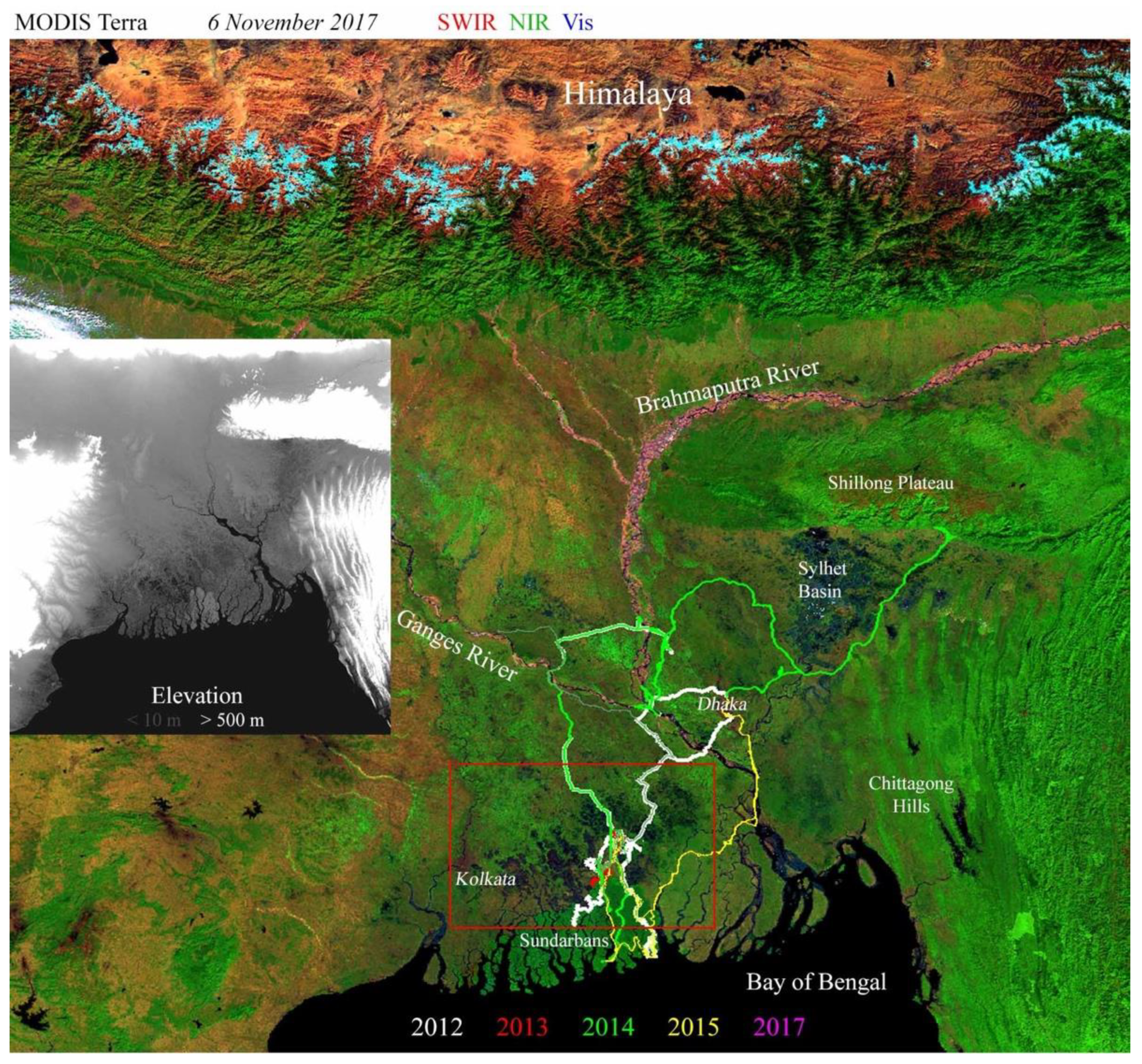
The South Asian monsoon drives both land surface phenology and data availability on the GBD. Extensive cloud cover is consistently present every year from May to September. When breaks in the clouds do occur, standing water is ubiquitous in the landscape below. The combination of these factors eliminates the utility of data from this time of year for reliable aquaculture mapping from optical imagery.

Rice is commonly planted during the monsoon and harvested late in the calendar year, generally November or December (the khareef crop). In some places, this cycle is made more complex with double or triple cropping. The Sundarbans mangrove forest is consistently green throughout the year.

Figure 4 shows a typical seasonal progression on the lower GBD using Landsat false color composite imagery from the 2016–2017 growing season. In these false color composites, the red channel of the image corresponds to reflectance in the shortwave infrared (SWIR), the green channel corresponds to the near-infrared (NIR), and the blue channel corresponds to the visible green wavelengths of light. All images are enhanced identically so colors are directly comparable between them. Displayed in this way, photosynthetic vegetation appears green because leaf mesophyll is highly reflective in the near-infrared and leaf chlorophyll is highly absorptive in the visible. Dry sediment and soil substrates appear red or brown because of the high shortwave infrared reflectance of most substrates. Water appears blue or black, depending primarily on depth and suspended sediment load, because water is highly absorptive at infrared wavelengths.

Immediately after the monsoon clouds clear, many areas are flooded—but not necessarily because of aquaculture. As the dry season continues, some flooded areas become covered with vegetation while others persist in being covered with standing water. For the Landsat analysis, we only compare dry season imagery (i.e., November–December) to provide a conservative estimate of the spatial extent of flooded ghers. For the analysis of MODIS time series, we compare interannual variations in vegetation extent on the mean date of maximum greenness (Julian day 314) in the post-monsoon period (October–December) when the rice crop reaches maximum canopy closure prior to senescence. The implicit assumption is that standing water observed at this time represents ghers not used for rice cultivation in that year.

3.2. MODIS-Derived Interannual Change, 1999–2017

MODIS EVI data were used to characterize the dominant spatiotemporal patterns in land surface phenology. In addition to providing the phenological setting for the Landsat observations, the EVI time series also reveal interannual trends in vegetation abundance and abrupt transitions between agriculture (annual cycle) and non-agriculture (no cycle) land use. While the 250 m spatial resolution of the visible and NIR bands of the MODIS sensor are nearly an order of magnitude coarser than those of Landsat, the frequent temporal revisit of MODIS makes it valuable for spatiotemporal analysis.

Figure 5 leverages this information to show the interannual mean (green) and variability (red + blue) of MODIS EVI imagery from a date in the middle of the post-monsoon rice season (JD 314, November 9 or 10), 2000–2016. Areas that are either green year-round (e.g., evergreen trees) or consistently cultivated (e.g., year-on-year agriculture) show as green on this image. In contrast, areas that undergo substantial change appear as magenta and consistently unvegetated areas show as black.

Individual MODIS pixel time series from select locations show the temporal complexity of the land use. Both the full MODIS 16-day composite time series (thin line) and the temporally sampled time series from only JD 314 of each year (thick line) are shown. The Sundarbans mangrove forest (1) was green year-long throughout the course of the study, though sometimes obscured by clouds. Regions of intense agricultural production (2) reach higher peak greenness values than Sundarbans, possibly due to less structural shadow in the agriculture canopies relative to the mangrove tree canopy. Both of these regions are consistently green on JD 314 and thus appear as green in Figure 5.

In May 2009, Cyclone Aila made landfall on the lower GBD, producing a storm surge of 130 cm to 260 cm above the coinciding tidal water levels [28]. The land surface inside the polders is generally below the mean river water level. Many embankments were breached as a result of the cyclone, and the land area within was flooded until the polders could be repaired and water pumped out [37]. In some regions, salinity issues caused difficulties with subsequent attempts at agriculture. As a consequence of these impacts, a spatially extensive region on the lower GBD was unvegetated for several years following the cyclone. Location (3) is an example of one such flooded region, which had recovered in greenness by the end 2016. The effects of Cyclone Aila will be demonstrated with greater spatial resolution later in the analysis.

Finally, agriculture–standing water transitions are shown as pixels that either converted during the study period (4) or were persistently covered in standing water since 2000 (5). These regions, as well as the Aila-affected regions, appear as magenta on Figure 5 since photosynthetic vegetation was recorded on JD 314 in some years between 2000 and 2016, but not in others.

This technique provides a means of concisely summarizing the expansion of standing water bodies in the MODIS era (2000–present). In addition, the MODIS time series demonstrates the feasibility of using November anniversary images to map flooded ghers, as they are clearly distinct from the other land cover types at that time of year. This knowledge is important for understanding the information present in the Landsat archive—a dataset with higher spatial resolution than MODIS, but significant aliasing in the temporal dimension.

3.3. Landsat-Derived Interannual Change, 1972–2017

The earliest portion of the Landsat image archive was acquired by the MSS instrument onboard the Landsat 1–3 satellites, corresponding roughly to the years 1972–1980. Data availability and quality are intermittent and highly geographically dependent for this portion of the archive. Landsat sensor design changed fundamentally between the MSS and TM instruments. While intercalibration of the TM/ETM+/OLI series of instruments is generally excellent, this level of quality cannot be extended to the MSS. This fact, in addition to the coarser spatial resolution and absence of the SWIR bands, fundamentally limits quantitative use for MSS data. Nevertheless, these data represent some of the earliest available multispectral imagery of the lower GBD and so offer valuable information—if understood with the appropriate caveats.

Figure 6 shows the earliest usable MSS image in comparison to a mosaic of one of the earliest usable pairs of TM images. The images have been enhanced to match as closely as possible, but care must be taken when visually comparing the colors of these images for the reasons given above. Nevertheless, qualitative examination of the images shows one important point—nearly as much standing water seems to be present in 1972 as in 1990. Some notable exceptions exist, including two large regions in the west of the study area, which consistently expand in later years. However, the largest region of standing water in 1972, near the center of the image, is covered with photosynthetic vegetation in 1990.

Similar results hold for 1975 and 1976 mid-dry season images (not shown). The remaining cloud-free MSS imagery was not acquired at comparable times in the growing season and so is not used in this analysis. The earliest TM image available is in 1987, resulting in a substantial data gap.

Conclusions about land cover dynamics in the early portion of the Landsat archive are thus fundamentally limited by extreme temporal aliasing. We cannot state with confidence the extent of land cover interconversion before 1987. However, visual interpretation of the data that we do have suggests that widespread, spatially extensive transitions from agriculture to aquaculture are unlikely to have occurred throughout the lower GBD in this time period due to the absence of large, spatially extensive areas of standing water in 1990.

Figure 7 shows changes in the extent of dry season standing water bodies in the lower GBD at 30 m resolution. The images shown in Figure 7 are false color composites with the same color channels as explained in Figure 4, with the exception of the 1975 image. This image was recorded by the Landsat 2 MSS and so, as stated above, has fundamentally different properties and must be interpreted with caution.

A clear, gradual increase in the spatial extent of flooded ghers is observed from 1990 up through at least 2010. This increase is consistent with anecdotal evidence collected in the field and previously published narratives. Regions identified from the MODIS imagery as decreasing in vegetation abundance show spatially coherent patterns of darkening consistent with the reflectance of decreasing areal vegetative cover and increasing abundance of standing water. This occurs on a broad scale across the lower GBD.

The difference between the 2010 and 2015 images, however, does not conform to the trend observed from 1990 through 2010. In several areas, locations covered by standing water in 2010 are revegetated in 2015. This could imply reconversion of aquaculture back to agriculture. Anecdotal evidence from field interviews supports the assertion that inhabitants of some regions are attempting to convert back to growing rice after failed attempts at aquaculture. Another plausible interpretation of the difference between the 2010 and 2015 images, however, could be the completion of multi-year rebuilding after the extensive flooding of Cyclone Aila in 2009. The effects of this cyclone are further shown below.

3.4. Cyclones on the Lower GBD

A total of 54 tropical cyclones have been recorded as making landfall in the northern Bay of Bengal between 1977 and 2010 [28]. One primary mechanism through which cyclones impact the landscape of the lower GBD is through their storm surge. The effect of this storm surge can be highly variable depending upon the timing of the storm in relation to the 2+ m tidal range present in the area, as well as whether the center of the storm tracks to the east or west of a specific location. For a detailed analysis of tropical cyclones on the lower GBD using tide gauge data, see [28].

These cyclones add a stochastic component to long-term land cover trends in the study area. The effect of this is illustrated using the example of Cyclone Aila, which made landfall in West Bengal on 25 May 2009. The storm surge from Cyclone Aila breached embankments and caused widespread flooding in the lower GBD, resulting in the displacement of >100,000 people. For more information about the effect of this cyclone, including geophysical and sedimentological analyses, see [37]. In contrast, Cyclone Sidr, which made landfall on 15 November 2007, produced a comparable storm surge, but had much higher wind speeds [28], which caused extensive defoliation in the mangroves and crop damage on the surrounding polders [57].

Figure 8 illustrates the effect of Cyclone Aila in the context of aquaculture. The top panel shows the landscape of the lower GBD in mid-May 2009, around two weeks before the cyclone made landfall. In contrast, the bottom panel shows the same landscape in early June 2009, approximately two weeks after the cyclone. The pervasive flooding that ensued is clearly evident from the Landsat imagery, as well as the MODIS time series presented above.

The dynamic nature of the landscape on the lower GBD must be accounted for when interpreting land use from optical satellite imagery, especially when performing retrospective analyses for which field validation is not an option. As Cyclone Aila shows, an aquaculture-dominated landscape may be optically indistinguishable from flooded agricultural fields. This non-uniqueness of the spectral signature of aquaculture is further discussed below.

3.5. Quantifying the Extent of Potential Aquaculture

Any attempt to map standing water from optical imagery must accommodate considerable spectral complexity. This complexity can arise from a number of physical processes, such as atmospheric effects, depth, sediment load, and the properties of the water surface. The top panels of Figure 9 illustrate this complexity.

In the simplest case, physical principles predict that the flowing tidal channels would entrain higher loads of suspended sediment than ghers with no appreciable overall flow direction or velocity. The higher suspended sediment load is then expected to scatter more visible and near-infrared light back into the aperture of the sensor, causing the river to appear brighter at those wavelengths than the standing water in the ghers. In many images, this chain of reasoning holds and the reflectance of the ghers is clearly distinct from that of the rivers. The upper left panel of Figure 9 illustrates this situation.

However, a number of complicating factors can introduce complexity to the scenario described above. Subtle atmospheric effects, common in the study area, can contaminate spectra in unpredictable ways, especially in the relatively short visible wavelengths, which carry the majority of the spectral signature from sediment load. In addition, flow in the tidal channels changes at different times each day, leading to essentially random sampling in tidal flow velocity from image to image. Seasonal variations in discharge of the main Ganges–Brahmaputra river channel also result in seasonal variations in sediment supply to the channels in the area. Furthermore, winds can roughen the water surface unpredictably, causing scattering and specular reflections that increase the apparent reflectance of the otherwise absorptive water. In addition, the reflectance of saturated soil, shallow (<~10 cm) standing water, and deeper ghers exists on a continuum with no clear decision boundary. All of these complexities can result in confusion during the step of inference when systematically categorizing pixels as river or gher. The situation in the upper right panel of Figure 9, while far from the worst case scenario, is common and presents a warning for overly confident classifications of aquaculture based on reflectance alone.

Fortunately, other data sources exist for the study area in addition to optical imagery. The Shuttle Radar Topography Mission (SRTM) used synthetic aperture radar (SAR) to develop a digital elevation model of much of the Earth’s land surface in early February 2000. The two Landsat images shown on the top panels of Figure 9 are the Landsat 5 acquisitions of the lower GBD during the time that SRTM was collecting data. SRTM elevations clearly distinguish water bodies as flat (lower left), allowing them to be easily classified by both elevation and slope (lower right). Using this additional information, we can compute the mean and dispersion of pixel reflectance spectra in areas mapped as river and ponds by SRTM, shown as insets to the upper panels of Figure 9.

This quantifies the scenario noted qualitatively above—the physical basis exists for spectral separability between ghers and other water bodies (upper left), but, in practice, the distinction is subtle and can often be confused when other complicating factors are at play (upper right). In a spectral mixture model, these variations in spectral separability are mapped into the uncertainty of fraction estimates. In order to accommodate the uncertainty that this complexity introduces, we use a range of fraction thresholds in the analysis that follows.

To derive quantitative estimates of the spatial extent of flooded ghers on the lower GBD, we perform a simple discrete classification on the Landsat image mosaics from November of each year with cloud-free imagery. After unmixing each image mosaic using the 3-endmember spectral mixture model described above, we then perform binary decision tree classifications by imposing band thresholds on the dark endmember fraction image. Because of the aforementioned uncertainty in equating high dark fraction values directly with aquaculture, we impose three fraction thresholds in order to generate conservative, moderate, and liberal estimates of the areal extent of standing water bodies. This approach leverages the robustness of SMA to provide land cover maps, which have the benefits of simplicity, transparency, and flexibility.

Figure 10 illustrates the effect of using a range of endmember fraction thresholds to generate maps of ghers potentially used for aquaculture. Liberal, moderate, and conservative decision boundaries were used to create binary maps denoting the presence or absence of ghers using 80, 85, and 90% subpixel dark fraction, respectively. Maps derived from the conservative decision boundaries can be interpreted as underestimating the total area of potential aquaculture. Likewise, liberal decision boundaries are designed to provide overestimates. For applications that have a physical basis for requiring fractional area of standing water, this method can be easily adjusted to tailor the result to the specifications of the user.

3.6. Quantitative Estimates of Dry Season Gher Extent on the Lower GBD

Total gher area is clearly a parameter of interest in this study because it quantifies their overall spatial extent at every time step. In addition, the size distribution of ghers is also important to understand, particularly as large-scale intensive aquaculture expands and communities transition to and from agriculture at individual plot scales. Changes in the size distribution and spatial connectivity of ghers inform both of these questions. The use of three fraction thresholds addresses the spectral uncertainty in estimating the areal extent of ghers. However, uncertainty exists in the spatial domain as well. As apparent from Figure 10, large, spatially contiguous areas of ghers are more likely to be reliably mapped than localized areas corresponding to a small number of Landsat pixels. Additionally, size distributions of spatially contiguous patches of land cover are often heavy-tailed [58], so small areas tend to be abundant and can significantly impact the overall sum.

One means of transparently presenting classification results given this knowledge is the rank-size plot. To generate these plots, a classified image is segmented into spatially contiguous regions. The area of each region is then computed and these areas are plotted in sequential order from largest to smallest. Because the area of the largest segment is generally several orders of magnitude larger than the area of the smallest segment (and there are often thousands of segments), these plots are conveniently displayed on logarithmic axes. The total area of segments larger than a given size threshold can be easily computed with a cumulative sum function, allowing complete transparency and flexibility to the needs of the user.

Figure 11a shows rank-size plot results for applying decision boundaries of 0.80, 0.85, and 0.90 dark fraction to the total area within the poldered region of Bangladesh. A minimum segment size of 9 pixels (8100 m²) was used. Conservative thresholds (blue) result in smaller individual segment sizes for each rank than moderate (green) or liberal (red) thresholds. Cumulative sums of these rank-size plots are shown in Figure 11b. This provides a means of ensuring that total area classifications are comparable.

Figure 11a,b is divided into columns corresponding to the maximum limiting spatial extent allowed for each analysis. The left column corresponds to only the area within the SRTM classification mask of Figure 9 (extremely conservative). In comparison, the center column uses the area of administratively defined Bangladeshi polder boundaries (moderate), while the right column uses the entire region of the Landsat mosaic with only a simple river mask imposed (liberal). For brevity, we will focus our discussion in this work on the results for the area delineated by the Bangaldeshi polders (center columns), although all three categories of result are presented for comparison.

For the conservative and moderate thresholds, the total area of ghers is observed to increase monotonically from 1990 to 2015. Examination of the rank-size plots shows both an increased total number of segments and growth of individual segments. Interestingly, cumulative sums of the liberal threshold show more area in 2010 than 2015. This is consistent with our qualitative observations from Figure 7, and may be due to the liberal threshold overestimating area of ghers by including areas still flooded by Cylone Aila. The polders surrounding these areas could have been breached still in 2010, but repaired by 2015.

The question of the spatial scale of contiguous regions of aquaculture can be conceptualized with the idea of spatial networks. Under this framework, a given type of land cover (e.g., flooded ghers) consists of spatially separated clusters, or network components. As the landscape evolves through time, these components can grow (or shrink), and merge (or divide). Slopes of the rank-size plots are estimated using the method of [59]. Cutoffs indicate the minimum segment size for which a linear fit is statistically defensible. The slope and curvature (or linearity) of the plots gives an indication of the fractional area of the total network represented by large versus small gher clusters. Steeper slopes and/or more pronounced downward curvature in the lower tail of the distribution indicate more area distributed towards larger clusters, and vice versa. For more background about rank-size distributions and spatial networks of land cover, see [60,61].

4. Discussion

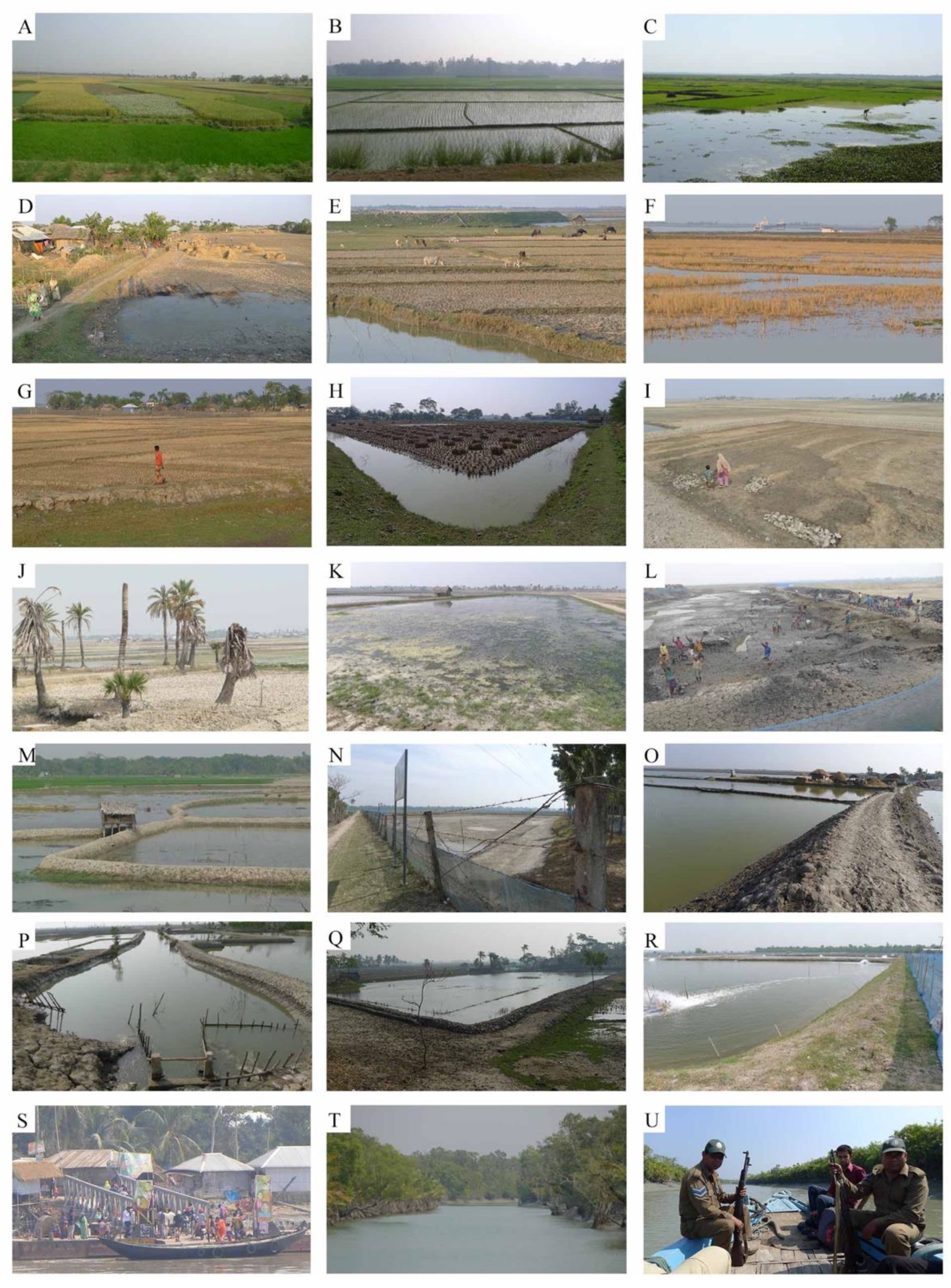
The lower GBD is a dynamic setting with extensive human modification. The broad diversity of land uses results in an intricate mélange of land cover continua. The complexity of the situation on the ground, alluded to by the field photos in Figure 2, must be considered when approaching the discrete classification of satellite imagery. In the parlance of satellite image analysis, nearly every pixel is mixed and the constituents of interest can have non-unique spectral signatures, as seen in Figure 8. Caution is advised.

Despite these complications, however, the careful analysis of multitemporal optical satellite imagery can yield informative results. MODIS imagery with relatively coarse spatial resolution but daily revisit time can be used to document, and control for, the predictable seasonal changes in vegetation phenology and land cover. Once this is understood, the higher spatial resolution and longer mission history of the Landsat sensor can be exploited profitably to provide more confident retrospective inferences of land cover at the 30 m scale.

It is clear that the spatial extent of ghers on the lower GBD has expanded considerably over the last several decades. From 1972 to 1990, changes in the spatial pattern of ghers can be observed but little change appears to have occurred in the overall spatial extent on the scale of Landsat imagery. Between 1990 and 2010, however, our observations clearly show ghers to have expanded rapidly on the lower GBD. This expansion appears to have slowed since 2010, in part because several polders flooded during Cyclone Aila have gradually returned to agriculture.

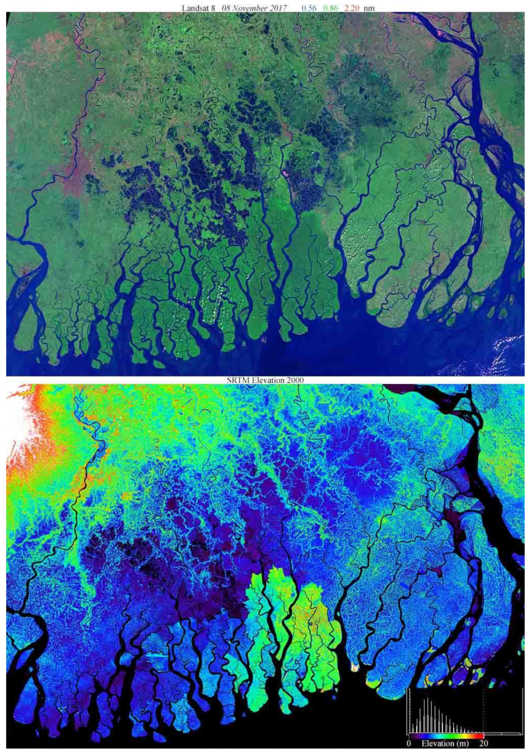
The state of land cover on the lower GBD circa 2017 is summarized in Figure 12. The top Landsat image mosaic, from November 2017, highlights the contrast between the current extent of ghers (black) and post-monsoon agriculture (light green)—although transitional areas remain an important source of uncertainty. With sufficient contrast enhancement of the color–elevation scale, the SRTM-derived digital elevation model clearly distinguishes between the land/water surface within the polders (blue/black) and the height of the tree canopy on embankments (green). The height of the Eastern Sundarbans mangrove forest is also clearly distinct in this pair of images. The Landsat images represent the mangrove forest as dark green because of canopy shadowing, and the elevation model captures the widely variable height of the canopy as a range from 4 to 20 m in elevation. Mangrove tree height and canopy density generally decrease from east to west as salinity increases with distance from the fresh water discharge from the main channel of the lower Meghna river east of the Sundarban.

The spatiotemporal dynamics of agriculture–aquaculture transitions on the lower GBD are applicable for a wide range of environmental and economic purposes. However, the success or failure of these applications is likely to hinge upon the case-by-case use of the land cover observations. For this reason, we hesitate to report a single parameter for physical processes that are inherently continuous (i.e., the area of ghers present in a given year). Instead, we choose to present the process of estimation of this parameter as transparently as possible, to give potential users an understanding of the tools, decisions, and uncertainties necessary to determine to meet their situation-specific needs. For the purpose of illustration, however, we provide a sample set of numbers based on a moderate choice of threshold and minimum segment size. For instance, within the Bangladeshi administrative polder boundaries, and using the moderate 85% dark fraction threshold, the overall extent of ghers appears to have increased from 290 km² in 1990 to 1459 km² in 2015. However, the more liberal 80% threshold shows an increase from 479 km² to 2031 km² in 2010, followed by a decrease to 1888 km² in 2015. The latter decrease is likely also partially a result of areas flooded during Cyclone Aila in 2009 returning to agriculture since 2010.

In addition, the distribution of standing water between large, homogenous clusters and small, separated ghers can be represented using the conceptual framework of evolving spatial networks. The slope and curvature of each of the rank-size plots used in this analysis directly show the size distribution of the spatial network at each interval of time. Viewed from top to bottom, each column of Figure 11 presents a condensed view of the relative contribution of large versus small gher clusters to the total area of the network. Viewed from left to right, each row of Figure 11 presents the difference between three limiting extents for these spatial networks. While a detailed network analysis is beyond the scope of this work, it is interesting to note that the rank-size distributions in this study show substantially steeper slopes than the global results for forests and agriculture found in [58] and the regional results for specifically agricultural networks in [61]. Steeper slopes imply greater areas of larger interconnected networks of ghers than smaller, more isolated ghers. The rank-size distributions in this study often feature prominent downward curvature in the upper tail, indicating that the largest segments are still smaller than would be expected if the distribution were generated by similar rates of nucleation, growth, and interconnection of gher-dominated areas. This is not present in either of the previous two studies and may be a result of the rigid physical constraints imposed on the network structure by the geography of the river channels and polders, limiting the interconnection of ghers.

The methods advanced in this study extend both the SAR-based methodology advocated by [25,62] and the optical understanding outlined by [20] and implemented in studies including [23,63]. To our knowledge, the extension of the spatial contiguity and patch size distribution analytic approach of [60] to aquaculture is novel. This approach is particularly interesting in the context of field-based studies such as [64], which present independent observations of size classes and the spatial distribution of ponds within administrative blocks. A particularly interesting avenue of future work could be to evaluate the feasibility of this approach in other mangrove-adjacent aquaculture systems—for instance, as studied by [65,66] in Latin America.

Moving forward, new data streams now available from both the public (e.g., ESA’s Sentinel 2) and private (e.g., Planet Inc., Victoria, BC, Canada) sectors have the capability to augment the Landsat record for continued monitoring efforts with enhanced spatial and temporal resolution. Despite these advances, however, the frequency of temporal sampling of optical imagery in South Asia is ultimately limited by cloud cover. Fundamental advances in land cover monitoring in monsoon-impacted field areas moving forward will require multisensor approaches that integrate passive optical imagery with SAR and thermal imaging, as well as field-based sensor networks.

Finally, the approach that we have developed for mapping standing water bodies on the basis of spatiotemporal characterization of the landscape is intentionally general. While our results apply specifically to one location, the fundamental physical principles that underlie our method can be easily ported to other landscapes where developing rigorous historical and current estimates of the spatial extent and size distribution of aquaculture is of interest. This is further enabled by the free global availability of decades of intercalibrated, geolocated multispectral satellite imagery at 30 m resolution from the Landsat program.

5. Conclusions

Standing water bodies on the lower GBD appear to have expanded considerably since the first available Landsat MSS image of the area in 1972. The spatial pattern of ghers reorganized, but was not observed to expand significantly, between 1972 and 1990. Between 1990 and 2010, a rapid expansion of dry season standing water was observed across the study area. This expansion appears to have slowed since 2010.

Considerable spatial and spectral complexity is present in the optical satellite imaging of ghers in this study area. This complexity results in uncertainty in the inference of quantitative estimates of the spatial extent of ghers. In order to explicitly address this uncertainty, we do not report a single number for the area of ghers at each time. Instead, we use a set of estimates to convey the range of outcomes that would result from conservative, moderate, and liberal approaches to mapping. Using the moderate approach, we find the area of ghers potentially used for aquaculture within the administrative boundaries of the Bangladeshi polders to have increased from roughly 290 km² to 1460 km² between 1990 and 2015.

References

1. Páez-Osuna, F. The environmental impact of shrimp aquaculture: A global perspective. Environ. Pollut. 2001, 112, 229–231. [Google Scholar] [CrossRef]
2. Froehlich, H.E.; Gentry, R.R.; Rust, M.B.; Grimm, D.; Halpern, B.S. Public Perceptions of Aquaculture: Evaluating Spatiotemporal Patterns of Sentiment around the World. PLoS ONE 2017, 12, e0169281. [Google Scholar] [CrossRef] [Green Version]
3. Primavera, J. Socio-economic impacts of shrimp culture. Aquac. Res. 1997, 28, 815–827. [Google Scholar] [CrossRef]
4. Hossain, S.; Eigenbrod, F.; Johnson, F.A.; Dearing, J. Unravelling the interrelationships between ecosystem services and human wellbeing in the Bangladesh delta. Int. J. Sustain. Dev. World Ecol. 2016, 24, 120–134. [Google Scholar] [CrossRef] [Green Version]
5. Paprocki, K.; Cons, J. Life in a shrimp zone: Aqua- and other cultures of Bangladesh’s coastal landscape. J. Peasant Stud. 2014, 41, 1109–1130. [Google Scholar] [CrossRef] [Green Version]
6. Shamsuzzaman, M.; Islam, M.M.; Tania, N.J.; Al-Mamun, A.; Barman, P.P.; Xu, X. Fisheries resources of Bangladesh: Present status and future direction. Aquac. Fish. 2017, 2, 145–156. [Google Scholar] [CrossRef]
7. Swapan, M.; Gavin, M. A desert in the delta: Participatory assessment of changing livelihoods induced by commercial shrimp farming in Southwest Bangladesh. Ocean Coast. Manag. 2011, 54, 45–54. [Google Scholar] [CrossRef]
8. Toufique, K.A.; Belton, B. Is Aquaculture Pro-Poor? Empirical Evidence of Impacts on Fish Consumption in Bangladesh. World Dev. 2014, 64, 609–620. [Google Scholar] [CrossRef] [Green Version]
9. Islam, M.S. From pond to plate: Towards a twin-driven commodity chain in Bangladesh shrimp aquaculture. Food Policy 2008, 33, 209–223. [Google Scholar] [CrossRef]
10. Islam, M.S.; Wahab, M.A. A Review on the Present Status and Management of Mangrove Wetland Habitat Resources in Bangladesh with Emphasis on Mangrove Fisheries and Aquaculture. In Aquatic Biodiversity II; Segers, H., Martens, K., Eds.; Springer: Dordrecht, The Netherlands, 2005; pp. 165–190. ISBN 978-1-4020-4111-2. [Google Scholar]
11. E-Jahan, K.M.; Ahmed, M.; Belton, B. The impacts of aquaculture development on food security: Lessons from Bangladesh. Aquac. Res. 2010, 41, 481–495. [Google Scholar] [CrossRef]
12. Ali, A.M.S. Rice to shrimp: Land use/land cover changes and soil degradation in Southwestern Bangladesh. Land Use Policy 2006, 23, 421–435. [Google Scholar] [CrossRef]
13. Akber, A.; Islam, A.; Ahmed, M.; Rahman, M.; Rahman, M.R. Changes of shrimp farming in southwest coastal Bangladesh. Aquac. Int. 2017, 25, 1883–1899. [Google Scholar] [CrossRef]
14. Ahmed, N.; Demaine, H.; Muir, J.F. Freshwater prawn farming in Bangladesh: History, present status and future prospects. Aquac. Res. 2008, 39, 806–819. [Google Scholar] [CrossRef]
15. Datta, D.K.; Roy, K.; Hassan, N. Shrimp culture: Trend, consequences and sustainability in the South-Western coastal region of Bangladesh. In Management and Sustainable Development of Coastal Zone Environments; Ramanathan, A.L., Bhattacharya, P., Dittmar, T., Prasad, M.B.K., Neupane, B.R., Eds.; Springer: Dordrecht, The Netherlands, 2010; pp. 227–244. ISBN 978-90-481-3068-9. [Google Scholar]
16. Milstein, A.; Islam, M.S.; Wahab, M.A.; Kamal, A.H.M.; Dewan, S. Characterization of water quality in shrimp ponds of different sizes and with different management regimes using multivariate statistical analysis. Aquac. Int. 2005, 13, 501–518. [Google Scholar] [CrossRef]
17. Islam, M.S.; Milstein, A.; Wahab, M.A.; Kamal, A.H.M.; Dewan, S. Production and economic return of shrimp aquaculture in coastal ponds of different sizes and with different management regimes. Aquac. Int. 2005, 13, 489–500. [Google Scholar] [CrossRef]
18. Rahman, M.R.; Ando, K.; Takeda, S. Cost Analysis of the Shrimp-Based Cropping System in Coastal Bangladesh. Trop. Agric. Dev. 2013, 57, 77–85. [Google Scholar] [CrossRef]
19. Hickman, G.D.; Hogg, J.E. Application of an airborne pulsed laser for near shore bathymetric measurements. Remote Sens. Environ. 1969, 1, 47–58. [Google Scholar] [CrossRef]
20. Ackleson, S.G. Light in shallow waters: A brief research review. Limnol. Oceanogr. 2003, 48, 323–328. [Google Scholar] [CrossRef]
21. Kutser, T.; Hedley, J.; Giardino, C.; Roelfsema, C.; Brando, V.E. Remote sensing of shallow waters—A 50 year retrospective and future directions. Remote Sens. Environ. 2020, 240, 111619. [Google Scholar] [CrossRef]
22. Al Sayah, M.J.; Nedjai, R.; Abdallah, C.; Khouri, M. On the use of remote sensing to map the proliferation of aquaculture ponds and to investigate their effect on local climate, perspectives from the Claise watershed, France. Environ. Monit. Assess. 2020, 192, 301–317. [Google Scholar] [CrossRef]
23. Duan, Y.; Tian, B.; Li, X.; Liu, D.; Sengupta, D.; Wang, Y.; Peng, Y. Tracking changes in aquaculture ponds on the China coast using 30 years of Landsat images. Int. J. Appl. Earth Obs. Geoinf. 2021, 102, 102383. [Google Scholar] [CrossRef]
24. Kontgis, C.; Schneider, A.; Ozdogan, M. Mapping rice paddy extent and intensification in the Vietnamese Mekong River Delta with dense time stacks of Landsat data. Remote Sens. Environ. 2015, 169, 255–269. [Google Scholar] [CrossRef]
25. Ottinger, M.; Clauss, K.; Kuenzer, C. Large-Scale Assessment of Coastal Aquaculture Ponds with Sentinel-1 Time Series Data. Remote Sens. 2017, 9, 440. [Google Scholar] [CrossRef] [Green Version]
26. Steckler, M.S.; Akhter, S.H.; Seeber, L. Collision of the Ganges–Brahmaputra Delta with the Burma Arc: Implications for earthquake hazard. Earth Planet. Sci. Lett. 2008, 273, 367–378. [Google Scholar] [CrossRef]
27. Reitz, M.D.; Pickering, J.L.; Goodbred, S.L.; Paola, C.; Steckler, M.S.; Seeber, L.; Akhter, S.H. Effects of tectonic deformation and sea level on river path selection: Theory and application to the Ganges-Brahmaputra-Meghna River Delta. J. Geophys. Res. Earth Surf. 2015, 120, 671–689. [Google Scholar] [CrossRef]
28. Chiu, S.; Small, C. Observations of Cyclone-Induced Storm Surge in Coastal Bangladesh. J. Coast. Res. 2016, 321, 1149–1161. [Google Scholar] [CrossRef] [Green Version]
29. Ahasan, M.; Chowdhary, A.; Quadir, D. Variability and Trends of Summer Monsoon Rainfall over Bangladesh. J. Hydrol. Meteorol. 2010, 7, 1–17. [Google Scholar] [CrossRef] [Green Version]
30. Ahmed, R.; Karmakar, S. Arrival and withdrawal dates of the summer monsoon in Bangladesh. Int. J. Clim. 1993, 13, 727–740. [Google Scholar] [CrossRef]
31. Goodbred, S.L., Jr.; Kuehl, S.A. Floodplain Processes in the Bengal Basin and the Storage of Ganges—Brahmaputra River Sediment: An Accretion Study Using 137Cs and 210Pb Geochronology. Sediment. Geol. 1998, 121, 239–258. [Google Scholar] [CrossRef]
32. Brammer, H. Physical Geography of Bangladesh; The University Press Ltd.: Dhaka, Bangladesh, 2012; ISBN 984-506-049-8. [Google Scholar]
33. Brammer, H. Climate Change, Sea-Level Rise and Development in Bangladesh; The University Press Ltd.: Dhaka, Bangladesh, 2014; ISBN 984-506-141-9. [Google Scholar]
34. Brammer, H. Bangladesh: Landscapes, Soil Fertility, and Climate Change; The University Press Ltd.: Dhaka, Bangladesh, 2016; ISBN 978 984 506 235 0. [Google Scholar]
35. Small, C.; Sousa, D.; Yetman, G.; Elvidge, C.; MacManus, K. Decades of urban growth and development on the Asian megadeltas. Glob. Planet. Chang. 2018, 165, 62–89. [Google Scholar] [CrossRef]
36. Cox, W. Demographia: World Urban Areas 2017; Wendell Cox Consultancy: Belleville, IL, USA, 2017. [Google Scholar]
37. Auerbach, L.W.; Goodbred, S.L., Jr.; Mondal, D.; Wilson, C.A.; Ahmed, K.R.; Roy, K.; Steckler, M.; Small, C.; Gilligan, J.; Ackerly, B.A. Flood risk of natural and embanked landscapes on the Ganges–Brahmaputra tidal delta plain. Nat. Clim. Chang. 2015, 5, 153–157. [Google Scholar] [CrossRef]
38. Gopal, B.; Chauhan, M. Biodiversity and its conservation in the Sundarban Mangrove Ecosystem. Aquat. Sci. 2006, 68, 338–354. [Google Scholar] [CrossRef]
39. Ahmed, N.; Garnett, S. Sustainability of Freshwater Prawn Farming in Rice Fields in Southwest Bangladesh. J. Sustain. Agric. 2010, 34, 659–679. [Google Scholar] [CrossRef]
40. Pokrant, B. Brackish water shrimp farming and the growth of aquatic monocultures in coastal Bangladesh. In Historical Perspectives of Fisheries Exploitation in the Indo-Pacific; Christensen, J., Tull, M., Eds.; MARE Publication Series; Springer: Dordrecht, The Netherlands, 2014; Volume 12. [Google Scholar] [CrossRef]
41. Prodhan, S.; Nasreen, M. Impact of Shrimp Cultivation on Agriculture: A Study in Parulia Union of Satkhira District. Int. J. Environ. Agric. Res. 2016, 2, 33–42. [Google Scholar]
42. Paul, B.G.; Vogl, C.R. Impacts of shrimp farming in Bangladesh: Challenges and alternatives. Ocean Coast. Manag. 2011, 54, 201–211. [Google Scholar] [CrossRef]
43. Islam, S.M.D.-U.; Bhuiyan, M.A.H. Impact scenarios of shrimp farming in coastal region of Bangladesh: An approach of an ecological model for sustainable management. Aquac. Int. 2016, 24, 1163–1190. [Google Scholar] [CrossRef]
44. Philcox, N. An Application of Contingent Choice Modelling to Assess Environmental Management Options in the Shrimp-Mangrove System in the Indian Sundarbans. Master’s Thesis, Simon Fraser University, Vancouver, BC, Canada, 2006. [Google Scholar]
45. Knowler, D.; Philcox, N.; Nathan, S.; Delamare, W.; Haider, W.; Gupta, K. Assessing prospects for shrimp culture in the Indian Sundarbans: A combined simulation modelling and choice experiment approach. Mar. Policy 2009, 33, 613–623. [Google Scholar] [CrossRef]
46. Das, S.K.; Sarkar, A. Environmental Impact of Wild Shrimp Seed Collection with Non-Selective Gears on Coastal Aquatic Biodiversity. Bangladesh J. Fish. Res. 2009, 13, 55–64. [Google Scholar]
47. Hossain, M.S.; Uddin, M.J.; Fakhruddin, A.N.M. Impacts of shrimp farming on the coastal environment of Bangladesh and approach for management. Rev. Environ. Sci. Bio/Technol. 2013, 12, 313–332. [Google Scholar] [CrossRef]
48. Chander, G.; Markham, B.L.; Helder, D.L. Summary of current radiometric calibration coefficients for Landsat MSS, TM, ETM+, and EO-1 ALI sensors. Remote Sens. Environ. 2009, 113, 893–903. [Google Scholar] [CrossRef]
49. Sousa, D.; Small, C. Global cross-calibration of Landsat spectral mixture models. Remote Sens. Environ. 2017, 192, 139–149. [Google Scholar] [CrossRef] [Green Version]
50. Adams, J.B.; Smith, M.O.; Johnson, P.E. Spectral mixture modeling: A new analysis of rock and soil types at the Viking Lander 1 Site. J. Geophys. Res. Space Phys. 1986, 91, 8098–8112. [Google Scholar] [CrossRef]
51. Small, C. Multiresolution analysis of urban reflectance. In Proceedings of the IEEE/ISPRS Joint Workshop on Remote Sensing and Data Fusion over Urban Areas (Cat. No.01EX482), Rome, Italy, 8–9 November 2001; pp. 15–19. [Google Scholar] [CrossRef]
52. Small, C.; Milesi, C. Multi-scale standardized spectral mixture models. Remote Sens. Environ. 2013, 136, 442–454. [Google Scholar] [CrossRef] [Green Version]
53. Huete, A.; Justice, C.; Van Leeuwen, W. MODIS Vegetation Index (MOD13). Algorithm Theor. Basis Doc. 1999, 3, 295–309. [Google Scholar]
54. Huete, A.; Liu, H. An error and sensitivity analysis of the atmospheric- and soil-correcting variants of the NDVI for the MODIS-EOS. IEEE Trans. Geosci. Remote Sens. 1994, 32, 897–905. [Google Scholar] [CrossRef]
55. World Bank. CERP Bangladesh Project Performance Assessment Report; World Bank: Washington, DC, USA, 2005. [Google Scholar]
56. Song, C.; Woodcock, C.E.; Seto, K.C.; Lenney, M.P.; Macomber, S.A. Classification and Change Detection Using Landsat TM Data: When and How to Correct Atmospheric Effects? Remote Sens. Environ. 2001, 75, 230–244. [Google Scholar] [CrossRef]
57. Small, C.; Sousa, D. Spatiotemporal Characterization of Mangrove Phenology and Disturbance Response: The Bangladesh Sundarban. Remote Sens. 2019, 11, 2063. [Google Scholar] [CrossRef] [Green Version]
58. Small, C.; Sousa, D. Humans on Earth: Global extents of anthropogenic land cover from remote sensing. Anthropocene 2016, 14, 1–33. [Google Scholar] [CrossRef] [Green Version]
59. Clauset, A.; Shalizi, C.R.; Newman, M.E.J. Power-Law Distributions in Empirical Data. SIAM Rev. 2009, 51, 661–703. [Google Scholar] [CrossRef] [Green Version]
60. Small, C.; Sousa, D. Spatial Scaling of Land Cover Networks. arXiv 2015, arXiv:1512.01517v1. [Google Scholar]
61. Sousa, D.; Small, C. Spatial structure and scaling of agricultural networks. Remote Sens. Environ. 2016, 184, 615–627. [Google Scholar] [CrossRef] [Green Version]
62. Ottinger, M.; Clauss, K.; Kuenzer, C. Opportunities and Challenges for the Estimation of Aquaculture Production Based on Earth Observation Data. Remote Sens. 2018, 10, 1076. [Google Scholar] [CrossRef] [Green Version]
63. Ren, C.; Wang, Z.; Zhang, Y.; Zhang, B.; Chen, L.; Xi, Y.; Xiao, X.; Doughty, R.; Liu, M.; Jia, M.; et al. Rapid expansion of coastal aquaculture ponds in China from Landsat observations during 1984–2016. Int. J. Appl. Earth Obs. Geoinf. 2019, 82, 101902. [Google Scholar] [CrossRef]
64. Ghosh, T.; Pramanik, N.; Das, S.; Chanda, A.; Mukhopadhyay, A. Spatial distribution of ponds in the indian sundarbans biosphere reserve: Special emphasis on size-class. In Practical Hydroinformatics; Springer: Singapore, 2021; pp. 21–43. [Google Scholar]
65. Tobey, J.; Clay, J.; Vergne, P. Maintaining a Balance: The Economic, Environmental and Social Impacts of Shrimp Farming in Latin America; Coastal Resources Center, University of Rhode Island: Narragansett, RI, USA, 2017; Available online: https://www.crc.uri.edu/download/MAN_0032.pdf (accessed on 1 January 2021).
66. Lacerda, L.; Borges, R.; Ferreira, A.C. Neotropical mangroves: Conservation and sustainable use in a scenario of global climate change. Aquat. Conserv. Mar. Freshw. Ecosyst. 2019, 29, 1347–1364. [Google Scholar] [CrossRef]
Figure 1. Index map of the Lower Ganges–Brahmaputra Delta (GBD) and surrounding area. Red box encompasses the study area. Inset elevation map emphasizes the subsidence of the polders northwest of the Sundarban forest. GPS tracks from field validation campaigns show the extent of river networks throughout the lower delta. False color composite: red = SWIR reflectance; green = NIR reflectance; blue = visible reflectance (MODIS bands 7, 2, and 4).
Remotesensing 13 04799 g001
Figure 2. Field photos of land cover in the dry season (January–March) collected by the authors on 5 campaigns over the years 2012–2017. Double cropped agriculture (AC) is present, as well as dry and inundated rice stubble (DH). Soil salinization and attempts to reconvert back to agriculture from aquaculture (IK), as well as various aquaculture methods (LR) are clearly evident. Substantial economic activity occurs on the waterways surrounding the polders (S). The biodiversity hotspot of the Sundarbans mangrove forest (T,U) directly abuts the polders.
Remotesensing 13 04799 g002
Figure 3. Calendar plots showing temporal distributions of cloud-free (green), partial cloud (yellow), and cloud-contaminated (red) Landsat imagery for the study area over nearly 30 years of Landsat TM, ETM+, and OLI acquisitions. The persistent cloud cover during the monsoon season is evident in the nearly complete absence of cloud-free images in the months of June, July, August, and September.
Remotesensing 13 04799 g003
Figure 4. Single year (2016–2017) vegetation phenology on the lower GBD. MODIS 16-day composite EVI pixel profiles show temporal patterns and Landsat 8 OLI false color composites show corresponding spatial detail. A wide range of land uses and phenological patterns are present. Rivers (A) and persistent aquaculture (F) have similar EVI time series, but can easily be distinguished spatially through a river mask. Note also seasonal changes in river reflectance compared to darker ponds, and the draining of many ponds in December and January. Single crop (B) and double crop (C,D) agriculture is also present on the lower GBD. Sundarbans mangrove forest (E) is evergreen, although sometimes obscured by cloud. Imagery for the subsequent portions of the study was chosen to be in the early dry season (November–December) in order to maximize the contrast between aquaculture and the various agricultural land cover types. All satellite images are false color composites: red = SWIR reflectance; green = NIR reflectance; blue = visible reflectance (Landsat 8 OLI bands 7, 5, and 3).
Remotesensing 13 04799 g004
Figure 5. Changes in post-monsoon land cover on the lower GBD 1999–2016, as imaged by MODIS. Image shown is a false color composite in which the green channel represents the temporal average (mean) and the red and blue channels both represent the variability (standard deviation) of MODIS EVI for JD 314 in each year, showing overall abundance and variability in vegetative cover. Areas with persistently low EVI (black) or with highly variable EVI (magenta) indicate presence of aquaculture and/or flooding. A number of areas were visibly impacted after Cyclone Aila in 2009. Administrative boundaries of Bangladeshi polders are shown in white. International Bangladesh/India border shown in yellow. All EVI time series plots are scaled from 0 to 0.8.
Remotesensing 13 04799 g005
Figure 6. Comparison of 1972 and 1990 land cover on the lower GBD. The 1972 image was acquired by Landsat 2 MSS. This instrument did not image in the SWIR and is not so rigorously intercalibrated as the later Landsat 4–8 TM/ETM+/OLI imagery. Both images are false color composites. For the Landsat 2 image, red = visible red reflectance; green = NIR reflectance; blue = visible blue reflectance (MSS bands 5, 6, and 4). For the Landsat 5 image, red = SWIR reflectance; green = NIR reflectance; blue = visible reflectance (TM bands 6, 4, and 2). The images were enhanced so as to be visually comparable, but the enhancements are not identical so the colors cannot be directly related across images. Regardless, broad-scale land cover can be assessed. While exceptions exist, there is clearly at least as much standing water in 1972 as in 1990. Few large, spatially coherent regions of standing water can be identified in 1990 that do not also exist in 1972. Systematic, widespread expansion of aquaculture before 1990 is not apparent.
Remotesensing 13 04799 g006
Figure 7. Dry season false color composite images of the lower GBD acquired by MSS, TM, ETM+, and OLI sensors onboard Landsat 2–8. Starting with 1990, spatially coherent expansion in extent of standing water clearly occurs over large portions of the lower GBD. Between 2010 and 2015, reconversion is observed in some areas as land cover transitions from aquaculture back to green vegetation. Both progressive and abrupt changes exist. Some regions gradually expand in spatial extent of dry season aquaculture, while others transition rapidly to their full area. Both smallholder and large, industrial-scale aquaculture operations are present. All images are false color composites. For the 1975 images, red = visible red reflectance; green = NIR reflectance; blue = visible blue reflectance (MSS bands 5, 6, and 4). For the 1990–2015 images, red = SWIR reflectance; green = NIR reflectance; blue = visible reflectance (TM bands 6, 4, and 2 or OLI bands 7, 5, and 3).
Remotesensing 13 04799 g007
Figure 8. Flooding and soil saturation shortly before and after Cyclone Aila made landfall in West Bengal on 25 May 2009. Landsat composites show increased area of inundation as black and saturated soils as dark green/brown. Inset shows water levels (red), modeled tides (green), and storm surge residual (blue) at nearby tide gauges from Chiu and Small (2016). Both images are false color composites: red = SWIR reflectance; green = NIR reflectance; blue = visible reflectance (TM bands 6, 4, and 2).
Remotesensing 13 04799 g008
Figure 9. Comparison of river and pond reflectance at the beginning and end of the SRTM mission in February 2000. On 11 February, river water reflectance was >1 σ brighter in visible/NIR bands than pond water (upper left) but, by 20 February, the river water reflectance distribution overlapped that of pond water at all wavelengths (upper right). SRTM elevations (lower left; single channel grayscale) clearly distinguish water bodies as flat, allowing them to be classified by both elevation and slope (lower right) to select spectra. Landsat 5 images (top row) are false color composites: red = SWIR reflectance; green = NIR reflectance; blue = visible reflectance (TM bands 6, 4, and 2). Lower right image is a discrete classification with colors chosen to emphasize contiguous clusters.
Remotesensing 13 04799 g009
Figure 10. Effect of thresholding Landsat dark fraction imagery using a range of values. Landsat endmember fraction image (left, false color composite: red = substrate fraction; green = vegetation fraction; blue = dark fraction) is thresholded using dark fraction values of 0.80, 0.85, and 0.90, corresponding to liberal, moderate, and conservative thresholds, respectively. Extent and spatial configuration of classified pixels varies substantially based on choice of decision boundary (right, false color composite: red = conservative; blue = moderate; green = conservative threshold). In addition, smaller contiguous areas clearly have lower confidence than larger, spatially homogenous regions of extensive aquaculture.
Remotesensing 13 04799 g010
Figure 11. (a) Evolution of aquaculture spatial networks between 1990 and 2015. Three different regions were used for this analysis: locations classified as ponds in February 2000 by SRTM slope and elevation (left column), regions within the administrative units of Bangladeshi polders (center column), and a large region of the lower delta with only rivers and ocean masked out (right column). Dark fractions for each image were segmented at thresholds of 0.80 (red), 0.85 (green), and 0.90 (blue). One-to-one lines shown in gray. Note logarithmic axes. (b) Evolution of cumulative size distributions of aquaculture spatial networks between 1990 and 2015. The same three regions and dark fraction thresholds were used as in Figure 10a. Overall sums given in the upper left corner of each plot and indicated by horizontal lines. Cumulative distributions for the portion of the “River Mask Only” study area within Bangladesh shown in thin curves and lighter gray horizontal lines. Cumulative totals for the Bangladesh-only analysis given in the lower right corner.
Remotesensing 13 04799 g011aRemotesensing 13 04799 g011b
Figure 12. Current (circa 2017) post-monsoon agriculture and aquaculture distribution and elevation. Landsat 8 false color composite (top) shows strong contrast between aquaculture ponds (black) and post-monsoon agriculture (light green). SRTM elevations show a ~4 m discontinuity between polder/pond level (purple + blue) and tree canopy height (cyan + green) on embankments. Tree canopy in Sundarban forest ranges from 4 to 20 m by species. Top image is a false color composite: red = SWIR reflectance; green = NIR reflectance; blue = visible reflectance (Landsat 8 OLI bands 7, 5, and 3). (bottom) image is a single-band elevation image with color ramp shown in lower right.
Remotesensing 13 04799 g012
Publisher’s Note: MDPI stays neutral with regard to jurisdictional claims in published maps and institutional affiliations.