
Accuracy of Sentinel-1 PSI and SBAS InSAR Displacement Velocities against GNSS and Geodetic Leveling Monitoring Data


1
Institute of Atmospheric Sciences and Climate (ISAC), National Research Council (CNR), Via del Fosso del Cavaliere 100, 00133 Rome, Italy
2
General Directorate of Geography and Environment (DGGMA), National Institute of Statistics, Geography and Informatics (INEGI), Av. Heroe de Nacozari Sur 2301, Jardines del Parque, Aguascalientes 20276, Mexico
3
Italian Space Agency (ASI), Via del Politecnico snc, 00133 Rome, Italy
*
Author to whom correspondence should be addressed.
Remote Sens. 2021, 13(23), 4800; https://doi.org/10.3390/rs13234800
Submission received: 29 October 2021
/
Revised: 20 November 2021
/
Accepted: 22 November 2021
/
Published: 26 November 2021
(This article belongs to the Section Remote Sensing Image Processing)
Abstract
:Correct use of multi-temporal Interferometric Synthetic Aperture Radar (InSAR) datasets to complement geodetic surveying for geo-hazard applications requires rigorous assessment of their precision and accuracy. Published inter-comparisons are mostly limited to ground displacement estimates obtained from different algorithms belonging to the same family of InSAR approaches, either Persistent Scatterer Interferometry (PSI) or Small BAseline Subset (SBAS); and accuracy assessments are mainly focused on vertical displacements or based on few Global Navigation Satellite System (GNSS) or geodetic leveling points. To fill this demonstration gap, two years of Sentinel-1 SAR ascending and descending mode data are processed with both PSI and SBAS consolidated algorithms to extract vertical and horizontal displacement velocity datasets, whose accuracy is then assessed against a wealth of contextual geodetic data. These include permanent GNSS records, static GNSS benchmark repositioning, and geodetic leveling monitoring data that the National Institute of Statistics, Geography, and Informatics (INEGI) of Mexico collected in 2014−2016 in the Aguascalientes Valley, where structurally-controlled land subsidence exhibits fast vertical rates (up to −150 mm/year) and a non-negligible east-west component (up to ±30 mm/year). Despite the temporal constraint of the data selected, the PSI-SBAS inter-comparison reveals standard deviation of 6 mm/year and 4 mm/year for the vertical and east-west rate differences, respectively, thus reassuring about the similarity between the two types of InSAR outputs. Accuracy assessment shows that the standard deviations in vertical velocity differences are 9−10 mm/year against GNSS benchmarks, and 8 mm/year against leveling data. Relative errors are below 20% for any locations subsiding faster than −15 mm/year. Differences in east-west velocity estimates against GNSS are on average −0.1 mm/year for PSI and +0.2 mm/year for SBAS, with standard deviations of 8 mm/year. When discrepancies are found between InSAR and geodetic data, these mostly occur at benchmarks located in proximity to the main normal faults, thus falling within the same SBAS ground pixel or closer to the same PSI target, regardless of whether they are in the footwall or hanging wall of the fault. Establishing new benchmarks at higher distances from the fault traces or exploiting higher resolution SAR scenes and/or InSAR datasets may improve the detection of the benchmarks and thus consolidate the statistics of the InSAR accuracy assessments.
Keywords:
InSAR; GNSS; leveling; Sentinel-1; ground deformation; land subsidence; validation; PSI-SBAS inter-comparison; accuracy; Mexico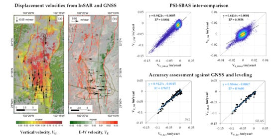
1. Introduction
Monitoring land changes and deformation is of paramount importance to understand solid Earth’s processes, especially those that are caused or exacerbated by anthropogenic activities and currently represent global challenges (e.g., [1,2]). Among the various surveying methods, two-pass and multi-temporal Interferometric Synthetic Aperture Radar (InSAR) techniques started to be exploited in the 1990s [3,4]. These techniques are now well-established and increasingly used by the geoscience community for scientific applications, as well as more operational tasks, such as monitoring and mapping services at a local to continental scale (e.g., [5,6,7,8,9,10]). They are also exploited by practitioners and professionals (civil protections, topographers/surveyors, geographers, engineers, oil and gas companies; e.g., [11,12]), with the aim to complement traditional methods based on geodetic surveying.
For a correct use of InSAR datasets, their quality must be assessed through the rigorous analysis of their precision and accuracy. The first is typically identified in terms of the standard error of the displacement estimates with respect to the linear model or the displacement velocity standard error. It depends on the quality of the scatterers (e.g., their coherence) and the number of available observations (e.g., [13,14,15]). On the other hand, accuracy indicates the systematic errors of InSAR estimates against the true values (or external independent measurements). It is usually evaluated by comparing InSAR products with independent geodetic monitoring data that are used as reference. As such, accuracy can inform about the capability of InSAR to provide reliable estimates on the deformation process under investigation.
Some studies analyzed the quality of Sentinel-1 InSAR-derived ground datasets and found evidence of achievable sub-centimeter accuracy for single displacement records in the time series, and sub-millimeter accuracy for annual displacement rates. These studies were based on tailored experimental setups with controlled displacements at artificial corner reflectors (e.g., [16,17]), investigation field sites monitored with continuous Global Navigation Satellite System (GNSS) stations (e.g., [18,19]), static GNSS surveying (e.g., [20]), or also using more extended geodetic leveling networks (e.g., [21]). By means of GNSS data, it was shown that the accuracy of Sentinel-1 InSAR time series against continuous monitoring records projected along the satellite Line-Of-Sight (LOS) is less than 8 mm [18] or even 5 mm [22], and that InSAR-derived vertical displacement velocities can differ by only a few millimeters per year against GNSS, even at fast subsiding sites [23].
Beyond the above cited papers, it is still rare to find in the literature studies where the accuracy of InSAR estimates is addressed. This work aims to contribute to the discussion in this field, to provide further evidence on the reliability of InSAR-derived displacement velocity estimates, as well as key limitations that should be accounted for when using these methods and datasets for land deformation monitoring. To achieve this goal, we selected the Aguascalientes Valley in central Mexico (Figure 1), an 80 km-long tectonic graben delimited by a system of N-S oriented normal faults [24]. Its unconfined aquifer system, which is formed by alluvial and fluvial graben-fill sediments, compacts as an effect of groundwater exploitation and piezometric level decline [25]. Surface faulting and fractures have developed in areas of greater differential settlement, inducing damage to urban infrastructure in both the capital city Aguascalientes and other towns and villages built across the valley, e.g., Jesús María and San Francisco de los Romo [26]. The widespread and well-marked land subsidence pattern and the range of deformation rates involved (reaching −150 mm/year along the vertical and ± 30 mm/year along the east-west direction [27]), provide an ideal setting for such an analysis.
Recent studies have used continuous GNSS data recorded at the two permanent stations that are deployed within the Aguascalientes Valley to understand the long-term behavior of the land subsidence process [28,29], and validate InSAR-derived estimates of vertical displacements and displacement rates [27,30]. Records at these stations have shown land subsidence rates as high as –90 mm/year, with significant trend variations in the medium and long-term [31]. Observed differences in the vertical rates estimated via Sentinel-1 InSAR and GNSS in 2015–2020 at these two stations were of only 0.1 and 0.5 mm/year [27], and at each epoch across the time series they were sub-centimetric [30]. However, such figures were based on a single or maximum two validation points only, in line with approaches used in other areas of interest worldwide. An improved understanding of the accuracy of InSAR estimates could be achieved by using an extended number of quality control points across the valley, also involving a wider range of vertical displacement rate values, not only within the main subsidence area, but also at its margins and beyond.
Geodetic data acquired by the National Institute of Statistics, Geography, and Informatics (INEGI) of Mexico over the last decades in Aguascalientes provide an exceptional dataset to trial such an assessment and validate InSAR-derived displacement velocities. Among its duties, INEGI is responsible for regulating and coordinating the national system of statistical and geographical information and for collecting and disseminating information about the territory. Its departments in charge of establishing and maintaining the geodetic reference frames regularly carry out precise geodetic leveling and GNSS surveys to densify the geodetic networks that provide the georeference base to support cartography, cadastral, and engineering projects. The maintenance of the reference frames includes geodetic surveys at network benchmarks to monitor ground deformation processes that affect the consistency of the networks. Some years ago, INEGI also started trialing InSAR methods to monitor land subsidence affecting major cities in central Mexico (e.g., [29,33]), towards embedding the technique into their geodetic methods to monitor deformation across the country.
A high-level comparison between the findings from the 1985–2004 traditional topographic surveys and Global Positioning System (GPS), and 2006–2015 static GNSS surveying on one side [33,34] and the 2015–2020 Sentinel-1 InSAR analysis on the other confirmed the agreement between the rates that were observed at a few locations across the valley [27]. However, the different time periods of the geodetic and InSAR datasets did not enable a rigorous quantitative comparison, given the marked non-linear deformation behavior that was recorded within the subsiding area and the temporally varying rates over the different years. Moreover, none of these studies on Aguascalientes assessed the quality and accuracy of the derived east-west displacement field map, which can be easily generated when InSAR output datasets from two viewing geometries, one in ascending and one in descending mode, are combined.
Beyond the Aguascalientes experimental test, the present research aims to bring in a contribution to the wider field of InSAR science and Sentinel-1 based investigations, given that until today, only a limited set of studies have attempted the analysis of the accuracy of InSAR-derived horizontal displacements (e.g., [16,35,36]). This lack of published studies persists, although the Sentinel-1 pre-defined observation scenario and rich data archive in both viewing modes (ascending and descending) covering a large proportion of the landmass [37] have boosted the opportunity for scientists and geodesists to generate east-west displacement rate products at different locations in the world where contextual geodetic data may be available for validation.
To contribute to addressing these knowledge gaps, in this paper, the accuracy of both the vertical and east-west displacement maps obtained from multi-temporal InSAR analysis are assessed using precise displacement records from long-term GNSS surveys at two permanent stations and tens of benchmarks, and from geodetic leveling on more than two hundred benchmarks deployed across the Aguascalientes Valley (Figure 1). To the best of our knowledge, this is the first time that an accuracy assessment has been done for the east-west displacement field, at least with such an extended number of validation points and data.
Both a low-pass and a full-resolution InSAR processing approaches were used to trial the assessment on two different spatial scales. Moreover, an inter-comparison between the output datasets from the low-pass and full-resolution InSAR analysis was carried out to verify the consistency between the output datasets and to understand any impact on the dataset quality due to the selected processing method. The drawbacks of the spatial resolution of InSAR datasets in relation to ground deformation rates that are rapidly varying in space are discussed. This is a key aspect of concern in faulted basins such as the Aguascalientes Valley, where the subsidence pattern is structurally controlled and shows significant horizontal gradients.
2. Materials and Methods
2.1. SAR Data and Multi-Temporal InSAR Processing
Two stacks of C-band Sentinel-1 SAR data were used for this research. The scenes were acquired with 5.405 GHz center frequency (i.e., 5.547 cm wavelength, λ) in right-looking mode, using the Interferometric Wide (IW) imaging mode. This is based on the Terrain Observation with Progressive Scans (TOPS) approach and uses LOS incidence angles (θ) varying from 31° (near range) to 46° (far range), i.e., ~39° at scene center. IW imagery is characterized by 250 km swath width, and 2.3 m pixel spacing in slant range and 14.1 m in azimuth, i.e., 5 m ground range and 20 m azimuth single-look resolution [38].
The two IW stacks that were used span the first two years of the Sentinel-1 mission from the beginning of operations until October 2016, and in particular include: 24 scenes acquired along descending track 114 in 25 October 2014–20 September 2016, and 22 acquired along ascending track 151 in 16 October 2014–29 October 2016 (Figure 1). Both were characterized by nominal site revisit of 12 days and VV single polarization, as per the predefined observation scenario over central Mexico during the operations ramp-up phase of Sentinel-1A, which began in late 2014 and lasted until October 2016 [39]. Despite the availability of a much longer series of Sentinel-1A and Sentinel-1B data acquired over the area of interest until today, the temporal coverage of the two stacks for this study was selected to match the period covered by the GNSS benchmark surveying and geodetic leveling. This was an important requirement to allow a fair and robust comparison and accuracy assessment (see Section 3.4), given that significant temporal variations were recorded in the surface deformation trend over the last decades from recent InSAR studies as well as at the permanent GNSS stations deployed within the valley [27,30,31].
The multi-temporal InSAR processing of the input stacks followed two main approaches, to gather a first low-pass assessment based on the Small BAseline Subset (SBAS) method [40] at medium resolution and then a spatially enhanced estimation based on the Persistent Scatterer Interferometry (PSI) approach [41]. The latter aimed to bring the analysis to the local scale and depict sharp velocity gradients where the displacement field changes very rapidly in space, for instance near and at the main faults.
The SBAS analysis exploited the Parallel-SBAS (P-SBAS) workflow by [22,42] and was run within ESA’s Geohazards Thematic Exploitation Platform (Geohazards TEP, also known as GEP) [43]. Image co-registration was implemented at single burst level and by guaranteeing accuracy in the order of 1/1000 of the azimuth pixel size. Interferograms were formed using short temporal baseline pairs, while the narrow orbital tube addressed the small perpendicular baseline requirement. Phase noise was reduced via 20 by 5 multi-looking in the range and azimuth directions, thus resulting in ~80–90 m ground pixels. Topographic phase components were subtracted from the interferograms based on the 30 m resolution Shuttle Radar Topography Mission (SRTM) digital surface model [44]. Studies conducted at other locations [23,45] proved the suitability of the above technical parameter settings in the GEP for land subsidence investigations. The workflow described in [22] was then followed to mosaic the burst interferograms to the sub-swaths and, afterwards, to the complete extent of the scene, carry out noise-filtering, select optimized triangular networks of interferograms, identify coherent targets, and estimate their LOS displacement rates (VLOS) and time series.
PSI processing was performed using the Stanford Method for Persistent Scatterers (StaMPS) software [46], while the steps of applying orbits, subswath splitting, coregistration, and interferogram formation of ascending and descending stacks were conducted in the Sentinel Application Platform (SNAP) v.8.0 using the S1TBX - ESA Sentinel-1 Toolbox [47]. The data for PSI processing was prepared using an amplitude dispersion index threshold of 0.42 [41], and for the phase noise estimation for the pixels in the interferograms a filter grid size of 30 m was applied. After the selection of the Persistent Scatterers (PS), the resampling of interferograms for phase unwrapping was done using a grid spacing size of 40 pixels in the input parameters to avoid phase unwrapping errors due to phase over-smoothing in pixels along the trace of the faults. Interferograms were corrected for spatially correlated look angle errors [48] and for linear tropospheric corrections, computed using the Toolbox for Reducing Atmospheric InSAR Noise (TRAIN; [49]) before phase unwrapping. Spatial (3D) phase unwrapping was performed using statistical models for cost functions in SNAPHU (Statistical-cost, Network-flow Algorithm for Phase Unwrapping; [50]).
The four output datasets (namely, two from the SBAS and two from the PSI analysis) were referenced to the same location in the eastern sector of the city (+21.854° N, −102.254° E; WGS84 datum), i.e., to the east of the Oriente fault, a zone that was typically adopted as reference in other InSAR studies, e.g., [51].
Separately for the SBAS and PSI results, the LOS displacement rates from the ascending and descending mode analysis were combined to estimate the vertical or up (VU) and the east-west (VE) deformation fields, under the assumption of negligible north-south deformation rates (VN), i.e., VN = 0. The latter was a generally suitable assumption, as the VN recorded at the two above mentioned permanent GNSS stations in Aguascalientes was an order of magnitude lower than VU and typically limited to ~2 mm/year in 2000−2020. The combination approach followed the workflow used for past studies in Aguascalientes and other Mexican cities [23,27,52], and is briefly recalled here for convenience of the readers (Figure 2). The VLOS from the ascending and descending mode results at each target i (VAi and VDi, respectively) were used to estimate its VUi and VEi as follows:
where Ei and Ui are the E-W and vertical directional cosines of the Sentinel-1 IW LOS at the position of target i in the ascending (A) and descending (D) mode, respectively. These can be computed as: Ei = −cosαisinθi, and Ui = cosθi, where αi is the heading angle of the satellite flight direction (Figure 2a,b). Their values will depend on the relative location of the target within the image footprint and its distance from the near and far range. Within the investigated area, the values of UAi range between +0.73 and +0.77, and UDi between +0.72 and +0.76, depending on the local value of θ, whereas EAi values range between −0.62 and −0.67 and EDi between +0.64 and +0.68, mostly controlled by the θ, as the cosine of the heading angles are very similar in the two geometries (but with opposite sign).
At locations where targets were identified from only one viewing mode, either ascending or descending, a simplified approach was used to estimate the VU, under the additional assumption that VE = 0:
2.2. GNSS Benchmark Monitoring and Data Processing
The two permanent GNSS stations in Aguascalientes city are INEG (+21.856° N, −102.284° E; Figure 3a), one of the National Active Geodetic Network (RGNA) stations operated by INEGI, and UAGU (+21.919° N, −102.315° E), a more recent station whose data is provided by the Trans-boundary, Land and Atmosphere Long-term Observational and Collaborative Network (TLALOCNet; [54]) operated by the Servicio de Geodesia Satelital (SGS) at the Instituto de Geofísica − Universidad Nacional Autónoma de México (UNAM) in collaboration with UNAVCO Inc. INEG station has provided relevant information about subsidence rates and its variability in time since its establishment in 1993 [33,34,55], and coordinate time series of both stations have been used as the most confidence geodetic data source to verify InSAR derived subsidence rates in Aguascalientes city. For a broader vision of the subsidence, prior to the implementation of InSAR techniques, a network of geodetic stations (Figure 3b,c) was established in the city, where periodic dual-frequency GPS repositioning campaigns have been performed since 2003 [34]; in the fall of 2006, the repositioning was extended adding new stations along the valley. In May 2016, the old GPS dual frequency receivers at INEG and the ones used for benchmark repositioning were replaced with new Leica GS14 GNSS multifrequency equipment that offers an accuracy for static surveying of 3 mm + 0.5 ppm in horizontal and 5 mm + 0.5 ppm (root mean square) in vertical. Static surveys at benchmarks were performed acquiring 2–3 h of observations; the length of the baselines formed from benchmarks to the permanent stations, INEG and UAGU, ranges between 1 and 50 km. GNSS measurements at the 82 benchmarks were suspended in fall 2016; the data used for this study are from survey campaigns that overlap with Sentinel-1 data availability, carried out in September 2014, January 2015, June 2015, October 2015, January 2016, June 2016, and October 2016. Benchmark distribution and the location of permanent stations are shown in Figure 1.
Previous calculations of subsidence rates at geodetic benchmarks were performed differentially post-processing the GNSS data in different International Terrestrial Reference Frame (ITRF) realizations using vendors software. For this study, data from static surveys were reprocessed in ITRF2014 [56], along with INEG, UAGU, and four other permanent GNSS stations (the nearest to the study area) using the software suite GAMIT/GLOBK v.10.71 [57]. Results from GAMIT/GLOBK differential processing showed accuracy improvement in north and east velocities for the monitoring benchmarks. In GAMIT/GLOBK, the velocities for INEG and UAGU were computed using daily data only for common periods of surveys at benchmarks, and its previous velocities from time series, for the period September 2014–October 2016, were affected by the antenna model change in May 2016; thus, harnessing all the data available for the period 2014−2016 and the quickness of the Precise Point Positioning (PPP) method [58,59], INEG and UAGU velocities for the period of interest were also calculated from PPP daily solutions using GPSPACE, developed by the Canadian Geodetic Survey (CGS).
Strategies for GNSS data processing included the use of satellite precise orbits [60], Earth orientation parameters, receiver and satellite clock corrections, absolute phase center variation models for receiver and satellite antennas [61,62,63], ocean and Earth tidal loadings, and corrections for atmospheric effects [64,65]. The accuracy of static GNSS surveys greatly depends on factors as positioning time, baseline length, and survey conditions, providing sub-centimeter to centimeter order accuracy in north and east, and height accuracies from 2 to 4 times the horizontal accuracy, depending also on processing procedures. Uncertainty of velocity estimates is reduced proportionally to the number of available measurements; mean 1 sigma uncertainties for east, north, and up velocities at the benchmarks, that account for at least five measurements, were 2.8, 2.6, and 11.3 mm/year respectively, while uncertainties for INEG and UAGU velocities were 0.2 and 0.3 mm/year in east, 0.1 and 0.2 mm/year in north, and 0.5 and 1.1 mm/year in height. In order to get only local horizontal velocities at GNSS permanent stations and benchmarks, comparable to InSAR north and east velocities, the plate velocity rates at each GNSS station in both components was subtracted from the GNSS velocity rates derived from coordinates time series. Plate velocity rates were computed using the ITRF2014 plate motion model [66].
2.3. Geodetic Leveling
In addition to repeated GNSS measurements, INEGI also performed yearly geodetic leveling surveys to monitor the vertical component of the deformation. Precise leveling surveys started in 2006 over some leveling lines across the city. The leveling surveys are performed using automatic digital levels and invar rods (Figure 4) and observing the standards for first order-class II procedures established in the Methodological Guide of the Vertical Geodetic Network [67], which consider double run survey of leveling lines.
The procedures before (instrument collimation), during (double run, alternated back and forward lectures, etc.), and after (orthometric correction and least squares adjustment) the measurements minimize the main sources of errors such as rod temperature and curvature and refraction errors as well as other systematic errors. The tolerance error for first order-class II survey of a section of 2 km (maximum) line length is 4 mm, and for an entire leveling line is 5 mm, where K is the length in kilometer units. Considering these tolerances and that in the leveling lines used for this study there are 1.5 benchmarks per km in average, this leads to estimated errors for benchmark heights of 2 mm as a maximum.
Leveling height velocities used for InSAR comparison at the location of the 202 benchmarks were estimated from surveys carried out during 2015 and 2016 using Leica DNA03 electronic digital levels and rods provided with invar bar code that allows a resolution of 0.01 mm in electronic height measurements, and offers a height accuracy of 0.3 mm (standard deviation) per 1 km double run measurements. The heights of leveling benchmarks of the vertical geodetic network are referred to the North American Vertical Datum of 1988 (NAVD88); for this study, the heights are propagated in the adjustment from benchmarks located outside the area affected by subsidence, where stability was verified through previous leveling surveys. The location of leveling benchmarks is shown in Figure 1. Fifteen of the leveled benchmarks also account for GNSS repositioning for the period September 2014–October 2016, yet the SBAS and PSI targets cover only ten of these benchmarks.
3. Results
3.1. Coverage of InSAR Outputs and Target Visibility
The fact that Aguascalientes state is located in a semi-arid region of Mexico may be considered as an advantage to apply InSAR methods. However, there are agriculture areas, mainly at the north of the valley, where interferograms are affected by low coherence; although scarce and small, there are also permanent vegetation areas where identification of reflective targets is limited.
The results after the multi-temporal InSAR processing show that within the state boundary (~5628 km2), the density of the retrieved coherent targets from the low-pass analysis with the SBAS method is on average 55 targets/km2 for each dataset, ascending and descending. These average figures account for not only the fact that sparse target networks are found in rural areas, but also that very dense target distributions are obtained within the capital city Aguascalientes, other towns, and bare lands within the state. In these zones, up to ~130 targets/km2 are retrieved (hence the maximum density that can be achieved with the ~90 m ground resolution of the output datasets). The PSI method enables the enhancement of the output targets density up to 790 PS/km2 on average across the state boundary. Maximum PS densities are achieved within the city, with up to 2696 PS/km2, while in general, the densities are ~740 PS/km2 within the valley and in the rural regions.
Regarding the geodetic benchmarks, the permanent stations (INEG and UAGU) are located over the roof of buildings with suitable reflectivity conditions for InSAR methods. This setup guarantees their coverage with results from both the SBAS and PSI analyses. Similarly, most of the geodetic stations used for GNSS monitoring surveys are covered as well, because they are located in urban areas and, usually, the sites chosen to establish GNSS stations are free from nearing objects that may obstruct or affect the signal emitted by GNSS satellites (e.g., trees and water bodies). Some GNSS stations in agriculture areas, where no targets were obtained in the SBAS processing, were discarded for the subsequent comparative analysis. On the other hand, even though the establishment of leveling benchmarks was not limited to sites away from trees, all of them were next to or along roads or streets whose reflective conditions were suitable for InSAR methods.
3.2. Observed Displacement Field
Minimum and maximum VLOS observed within the state with the SBAS analysis were −99 and +19 mm/year for the ascending dataset and −93 and +28 mm/year for the descending one. After the combination of the two datasets and the estimation of the vertical and east-west displacement rates (see Section 2.1), the observed minimum and maximum rates were –139 and +30 mm/year for the VU and −30 and +27 mm/year for the VE (Figure 5).
The VLOS observed within the state with the PSI method ranged between −113 and +40 mm/year for the ascending dataset and between −103 and +48 mm/year for the descending one. The combined dataset revealed minimum and maximum rates of −141 and +46 mm/year for the VU and −64 and +68 mm/year for the VE (Figure 6).
Both the SBAS and PSI output datasets clearly depict the land deformation pattern that affects the whole Aguascalientes Valley and is well-known from past InSAR investigations with SAR imagery from the ERS-1/2 [27], ENVISAT [27,28,33], ALOS-1 [51], TerraSAR-X [28,33], RADARSAT-2 [68], and Sentinel-1 [27,29,30] missions. The alluvium within the north-south trending graben rapidly compacts as a consequence of the overexploitation of groundwater resources from the Ojocaliente-Aguascalientes-Encarnación interstate aquifer in excess of recharge from rainfall [69]. The subsidence of the valley floor became apparent in the 1980s, associated with ground faulting and fissuring in zones of sharp spatial changes in the vertical deformation regime [26]. Two north-south elongated bands affected by east-west deformation towards the maximum subsidence locations (approximately, the center of the valley) were clearly detected in 2014−2016, confirming what was already detected in 2003−2008 by INEGI via static GNSS surveying [28] and, more recently, via 2015−2020 InSAR analysis [27].
Outside the main subsidence area, some atmospheric effects are visible in both the SBAS and PSI output datasets (Figure 5 and Figure 6). These are mostly observed in the ascending mode results, showing some areas with +5 to +10 mm/year displacement towards the satellite sensor. The two main factors that could play a role in this are on one hand, the limited number of input scenes in both viewing modes (i.e., 24 and 22), making atmospheric phase removal more challenging during the multi-temporal image processing and, on the other hand, the acquisition time of the Sentinel-1 data. In particular, images depicting Aguascalientes are acquired along descending orbits at ~12:40 UTC (i.e., at dawn, 7:40 a.m. local time), and along ascending orbits at ~01:00 UTC (i.e., at dusk, 8:00 p.m. local time), thus making the latter potentially more affected by ionospheric effects (e.g., [70]).
GNSS data show VU between −99 and +8 mm/year, with the highest negative velocities recorded in the north-western part of Aguascalientes city, then decreasing to −50 mm/year or less when moving towards the south-western sector (Figure 7a). To the east of the Oriente fault, VU values are limited to the range ±8 mm/year. Evidence from geodetic leveling is consistent with both the InSAR and GNSS observations, with the vertical rates observed in the surveyed area between −97 and +8 mm/year (Figure 7b).
The map of horizontal displacement rates retrieved using GNSS (Figure 8a) shows that the direction of most of them points towards the nearest maximum sinking areas. Displacement rates appeared most significant along the east-west direction, with recorded VE reaching −22 and +27 mm/year (Figure 8b). The negative peaks (displacements towards the west) were found in proximity to the Oriente fault where significant motion was recorded towards the center of the valley, generally with rates between −12 and −15 mm/year, and the minimum reached at benchmark FG19A. The positive peaks (displacements towards the east) were recorded close to the cluster of faults bounding the western sector of the city, namely San Marcos, Del Valle II - Pirules, Primo Verdad, and Colinas del Rio faults. In their proximity, movements were typically between +9 and +19 mm/year, while +27 mm/year was reached at benchmark FG24 near Crena fault.
North-south displacement rates were limited to the ±18 mm/year range, with most benchmarks recording less than ±5 mm/year, and only a few exhibiting higher rates (Figure 8a). These were in proximity to Crena (FG24 and FG24B, with VN of +10 and +18 mm/year, respectively), Del Valle II - Pirules (FG18, with +12 mm/year), and Vicente Guerro (FG28A, with +12 mm/year) faults, as well as at benchmarks FG25 (+18 mm/year) and FG22C (+17 mm/year) which were close to the Jardines-Lindavista fault in the southern sector, and to the Oriente fault at benchmarks FG09 and FG09A (see benchmark locations in Figure 1b). Negative VN were less frequent and were only recorded at benchmark FG21A near San Marcos fault (−18 mm/year) and FG26 at the hanging wall of the Oriente fault (−12 mm/year).
3.3. PSI-SBAS Inter-Comparison
Figure 9 shows the results of the PSI and SBAS comparison for the whole area of interest. The relative differences in the vertical and east-west velocity estimates provided by the two methods, ΔVU and ΔVE, were computed as follows:
The summary statistics from the comparison are reported in Table 1. Throughout the investigated area, the differences were within the −42 to +56 mm/year range for the vertical rates and −47 to +30 mm/year for the east-west rates, though the majority of the area showed differences in the range ±5 mm/year.
The highest differences were found mainly outside the valley and the main subsidence area, and appeared spatially correlated with the areas that were found most affected by partly uncompensated atmospheric phase components (see Section 3.2). As these were mostly outside the region that is covered by the geodetic data (see Figure 1), they should not notably affect the assessment when performing the comparison at the benchmark locations or when estimating accuracy (see Section 3.4).
Point-wise analysis at the 2 permanent GNSS stations and 62 GNSS benchmarks (Figure 10) revealed a very good agreement between the results retrieved using the two image processing methods and independent analyses with PSI and SBAS. The linear regression in Figure 10a shows an almost perfect match between the PSI and SBAS estimates of the vertical rates, with a regression approaching the 1:1 line and a determination coefficient R2 of ~0.96. Despite a slightly lower R2, the east-west rates also compare well and do not deviate much from the 1:1 line (Figure 10b). In this case, however, the range of values used for the comparison is limited to ±20 mm/year, with respect to the wider representation of rates that is provided by the vertical velocity field (up to −100 mm/year). The observed distributions of ΔVU and ΔVE are centered on 0 (Figure 10c,d), and generally do not highlight any correlation between the two variables (Figure 10e).
Only a few targets exhibited higher differences for both ΔVU and ΔVE, such as the targets at benchmark FG15A where ΔVU = −29 mm/year and ΔVE = −15 mm/year, and at benchmark FG09A where ΔVU = −19 mm/year and ΔVE = −6 mm/year (Figure 10e). These differences are probably related with the close proximity of the two benchmarks to the trace of the Oriente fault, indeed FG15A and FG09A are 15 m and 5 m off the trace, respectively (see Figure 1b and Figure 7). Similarly, ΔVU = +15 mm/year was observed at benchmark FG08A, located 3 m off the trace of the San Cayetano-Miravalle fault.
The most plausible reason for the occurrence of larger differences near the faults and fissures that are mapped within the valley might be linked to the difference in spatial resolution of the PSI and SBAS output datasets (i.e., ~30 m for the PSI output, and ~90 m for SBAS), hence in the exact ground location that is sampled by the two methods. In particular, the PSI and SBAS output targets may encompass different proportions of land, part belonging to the hanging wall and part to the footwall of these faults. Given that it is along the faults where the highest differences in rates occur (see Figure 5 and Figure 6), in these zones, the PSI and SBAS output targets may span ground deforming at different vertical and east-west rates and likely highlight higher differences during the inter-comparison.
By extending the inter-comparison to the full set of targets (Figure 11), the statistics further consolidated around an optimal match between the outputs from the two processing methods. The regression lines in Figure 11a,b deviate from the 1:1 line a bit more than what is observed from the limited sample of 64 targets at the GNSS stations and benchmarks only, though the data clouds reach maximum density at the 1:1 line, indicating an overall very high match between the PSI and SBAS outputs across the whole processed area. Similarly, histograms in Figure 11c,d and the comparison between ΔVU and ΔVE in Figure 11e confirm the remarkable match between the results from the different processing methods. Average differences between the rates estimated via SBAS and PSI analyses along both the vertical and east-west directions were sub-millimetric, i.e., on average −0.3 and −0.4 mm/year, respectively (Table 1). Similarly, the Root Mean Square Error (RMSE) improved from 7.0 to 6.3 mm/year for the vertical rates, and from 4.3 to 3.9 mm/year for the east-west rates.
3.4. Accuracy of InSAR Displacement Velocity
Provided that the exact and ‘true values’ of the deformation occurring across the valley cannot be measured by any survey or method (even the most advanced or accurate), the data gathered through the GNSS or geodetic leveling surveys can provide the best available accepted values that can be used as ‘reference’. Therefore, the differences ΔVU and ΔVE between the vertical and east-west velocities recorded by the reference dataset (from either GNSS or geodetic leveling) and those estimated via the InSAR analysis enable an assessment of the estimation errors (hence the inaccuracy) of the PSI and SBAS output datasets, and can therefore be used as a proxy to understand the accuracy of the Sentinel-1 InSAR datasets. These were computed as follows:
Vertical displacement velocity estimated using InSAR methods was found generally in agreement with geodetic observations. In Figure 12, the VU at 10 benchmarks that were surveyed using both GNSS repositioning (VU estimated from height time series) and geodetic leveling (VU based on two measurements with over 1 year-long difference, between April 2015 and October 2016) were compared with the estimates provided by InSAR using the PSI and SBAS methods. Very high match between the observations was found, with some discrepancies (e.g., at benchmarks FG09A and JM409) that can be explained by the proximity of the benchmarks to the main faults, as discussed in Section 3.3, as well as in more detail later in this section.
Table 2 and Table 3 summarize the key statistics obtained from the comparison of geodetic and InSAR estimates at the whole sets of surveyed points across the valley. The results highlight that, on average, the InSAR-derived VU differed from GNSS data by +4 mm/year (PSI) and +8 mm/year (SBAS), with a standard deviation of 9 and 10 mm/year, respectively. The associated RMSE was around 10 mm/year for the PSI dataset and 13 mm/year for SBAS. Similarly, the comparison with geodetic leveling data showed average differences of −3 mm/year for the PSI results and less than +1 mm/year for the SBAS results, both with a standard deviation ~8 mm/year. In both cases, the RMSE was ~8 mm/year. When comparing east-west displacement rates VE, average differences were sub-millimetric for both the PSI and SBAS results, in particular, −0.1 and +0.2 mm/year, respectively, both with a standard deviation of ~8 mm/year. Using both methods, the RMSE was ~8 mm/year.
The scatterplots and histograms in Figure 13 and Figure 14 provide a detailed overview of the comparisons and allow the identification of the level of fit of the InSAR estimates with the monitoring data from the GNSS surveys. The regression lines for the VU from both PSI and SBAS are characterized by slopes and R2 of ~0.9 (Figure 13a and Figure 14a), though slightly higher values were observed for the PSI analysis, likely due to the better spatial resolution of the PSI output dataset. On the other hand, the goodness of fit of the linear regression for the VE estimates was lower than that for VU, and the associated R2 dropped to 0.3 for the PSI analysis (Figure 13b), and 0.4 for SBAS (Figure 14b). Histograms in Figure 13d,g and Figure 14d,g show that the differences were mostly concentrated around 0, with a limited spread towards higher values (either negative or positive).
While there is no particular evidence of correlation between ΔVU with the magnitude of the VU estimated with the GNSS, i.e., VU_GNSS (Figure 13e and Figure 14e), it appears that ΔVE grew with increasing VE_GNSS for both the PSI and SBAS results (Figure 13h and Figure 14h), with R2 of ~0.63. This suggests that higher differences between InSAR and GNSS estimates of the east-west velocity were found for locations displacing faster. The observed discrepancies were also relatively moderate, with respect to the magnitude of the estimated rates. Indeed, the linear relationships indicated that ΔVE = 0.675×VE_GNSS − 0.07 mm/year for the PSI dataset, and ΔVE = 0.627×VE_GNSS + 0.3 mm/year for the SBAS dataset. This means that, for instance, at a location moving at −25 mm/year VE, around −17 mm/year velocity difference is expected between PSI and GNSS, and −15 mm/year between SBAS and GNSS. These correspond to relative errors (i.e., ΔVE/VE_GNSS) of 68% and 61%, respectively. More generally, for east-west displacement rates exceeding ±10 mm/year, the relative errors typically are around 67−68% for PSI, and 60−66% for SBAS.
No apparent trend or correlation could be observed when comparing ΔVU with ΔVE (Figure 13c and Figure 14c), or any of these against the displacement rates that were recorded along the north-south direction VN using GNSS (Figure 13f,i and Figure 14f,i). Nevertheless, at some benchmarks, there appeared to be a slight relationship between the occurrence of faster VN and higher ΔVU and/or ΔVE, indicating that higher errors in the estimation of the vertical and east-west displacement rates occur when the north-south displacement component is not negligible (hence, the assumption made during the ascending and descending outputs combination is not valid; see Section 2.1). For instance, at benchmark FG21A (located 7 m off the trace of San Marcos fault) where VN = −18 mm/year, the values of ΔVU and ΔVE from the SBAS analysis were respectively +14 and −11 mm/year (Figure 14f,i), and from the PSI analysis they are +2 and −14 mm/year (Figure 13f,i). Similarly, at benchmark FG26 (located in the hanging wall of the Oriente fault, 10 m off its trace), where VN = −12 mm/year, the values of ΔVU and ΔVE from the SBAS analysis were respectively +11 and −10 mm/year (Figure 14f,i), and from the PSI analysis they were +13 and −6 mm/year (Figure 13f,i). In any case, the distribution of the data in the scatterplots did not allow for a robust regression analysis to determine a good mathematical relationship between errors in the vertical or east-west rates with the north-south rates.
To quantify the magnitude of the contribution to the observed ΔVU and ΔVE that was made by the VN = 0 assumption, the GNSS measurements were used to run a simulation. The GNSS velocity vector [VE VN VU] at each benchmark i was first projected onto the Sentinel-1 LOS in the ascending and descending mode, by using the local values of the LOS directional cosines Ei, Ni and Ui (e.g., [52]; see also Figure 2c):
The two LOS projected values of the GNSS vector were then used to re-calculate VU and VE by exploiting Equations (1) and (2), under the VN = 0 assumption (as they were the values that InSAR could estimate by neglecting VN). The differences between the VU and VE measured with GNSS and their re-calculated values were then compared to the values of VN at each benchmark (Figure 15). The data suggest that the errors made when VN is omitted were approximately ΔVU = 0.1603 × VN mm/year and ΔVE = 0.0044 × VN mm/year. These indicate that, for VN in the range of ±18 mm/year (as observed in Aguascalientes; see Section 3.2), the expected magnitude of this contribution is no more than ±3 mm/year for VU and ±0.1 mm/year for VE.
Improved accuracy statistics were found when the VU from the InSAR analysis was compared with the geodetic leveling data (Figure 16). For both the PSI and SBAS methods, an improvement in the R2 was observed, reaching respectively 0.95 and 0.96. The linear regressions matched well with the 1:1 line (Figure 16a,d), and the residuals showed a distribution centered around 0 (Figure 16b,e) with limited deviation from the average values, as shown by the respective statistics in Table 2.
Differently from what was observed in the framework of the comparison with the GNSS data, there seems to be some correlation between the vertical velocities estimated via leveling VU_Lev and the amount of difference observed against them when using InSAR methods (Figure 16c,f). The data suggest that higher discrepancies between InSAR and leveling estimates were found for locations subsiding faster. The linear relationships indicate that ΔVU = 0.196 × VU_Lev + 1.6 mm/year for the PSI dataset and ΔVU = 0.218 × VU_Lev + 6.7 mm/year for the SBAS dataset. This means that at a location subsiding at −100 mm/year, around −18 mm/year velocity difference is expected between PSI and leveling, and −15 mm/year between SBAS and leveling. These correspond to relative errors (i.e., ΔVU/VU_Lev) of 18% and 15%, respectively. More generally, for locations subsiding faster than −15 mm/year, the relative errors are below 20% for both PSI and SBAS. For targets subsiding faster than −50 mm/year, the relative errors typically are expected to be around 16–19% for PSI, and 8–17% for SBAS.
4. Discussion
The statistics illustrated in Section 3 reassure both on the similarity in the output datasets from the SBAS and PSI analyses (despite the intrinsic different properties and processing steps of the two methods), and on the accuracy of InSAR datasets against geodetic measurements.
It is worth considering first the suitability of geodetic velocities to assess the quality of InSAR outputs, in relation to the accuracy that characterizes the estimates that are used as ‘reference’ for the comparison. On one hand, there is no doubt that the data from leveling and permanent GNSS stations have a suitable accuracy to act as reference, given that these showed maximum 2 mm heights errors from the leveling survey, and up to 0.5 and 1.1 mm/year VU uncertainties for the two permanent stations (see Section 2.2 and Section 2.3). The same applies to east-west and north-south velocities estimated from GNSS repeated measurements at the benchmarks, which showed less than 3 mm/year for VE and VN (see Section 2.2). However, this might not be the case for vertical velocities at benchmarks with a limited number of measurements used for the estimation (i.e., 5–7), resulting in accuracy of more than 10 mm/year (see Section 2.2). This aspect should be accounted for when the findings are used to establish the quality of the two InSAR output datasets and their relative errors.
The standard deviation values that were found from the PSI-SBAS inter-comparison and InSAR-geodetic data comparison reflect the discrepancies between the results obtained by the different methods and, as such, can be used as performance indicators for both assessments. The PSI-SBAS inter-comparison revealed a standard deviation of 6 mm/year for the vertical rates VU and 4 mm/year for the east-west rates VE (Table 1). Past InSAR method inter-comparisons, for instance [21], found standard deviations between 0.6 and 1.9 mm/year when assessing different PSI products generated by different providers using the same input ERS-1/2 and ENVISAT SAR data for a coal mining site affected by ground subsidence. Similarly, standard deviations of 1.1 mm/year were observed on average when comparing Sentinel-1 PS and distributed scatterers datasets generated by different providers in [71].
Although the indicators found in Aguascalientes seem to reveal a lower match between the results, these might be explained by (i) the fact that a low-pass (SBAS) and a point-wise (PSI) method are inter-compared in this study; (ii) the presence of some uncompensated atmospheric signals due to the relatively small number of input scenes processed; (iii) the limited length of the time series (e.g., 2 years for Aguascalientes, against 12 years in the work by [21]); and also (iv) the much wider range of displacement rates that are involved (up to −140 mm/year in Aguascalientes, against −20 mm/year in [21], and less in [71]), thus enlarging the value range used for comparison (and, potentially, the estimation differences). By restricting the range of displacement velocity values inter-compared in Aguascalientes to the same width examined in [21] (i.e., up to −20 mm/year VU), the standard deviation for the differences in the vertical rates drops by only 0.3 mm/year, suggesting that the first three factors probably play a major control on the statistics found. Among them, the number of scenes and the length of the time series could likely be the main drivers for the observed differences in accuracy. Indeed, these two factors are known for controlling the quality of the InSAR output datasets (e.g., [14,72]) and their ability to capture long-term deformation signals.
The accuracies found for the vertical rates estimated with PSI and SBAS (Table 2) were in the order of 9−10 mm/year against whole GNSS data, and below 8 mm/year against the leveling data. By referring only to the more accurate vertical rates from the two permanent GNSS stations, the accuracy improved to 6 mm/year for PSI and 7 mm/year for SBAS. The findings are consistent with observations by [21], who found standard deviations of PSI-derived vertical rates of up to 7 mm/year against leveling data. For the east-west rates, the accuracies against whole GNSS data were around 8 mm/year for both PSI and SBAS (Table 3), while when the comparison was limited to the two permanent stations, they dropped to 1 and 2 mm/year, respectively. In areas affected by north-south displacement, only up to ±3 mm/year vertical and ±0.1 mm/year east-west velocity differences between InSAR and GNSS were due to the assumption of null north-south velocities that is used during the ascending and descending dataset combination (see Section 2.1).
A large portion of the discrepancies found between InSAR estimates and geodetic data can be explained by the location of the benchmarks and their proximity to the faults. In many cases, benchmarks are deployed in pairs, one to each side of the fault trace, because they were originally established to monitor the behavior of the faults. Given their proximity, they often fall within the same SBAS ground pixel or closer to the same PSI target, hence are associated with the same displacement rate value from the InSAR analysis, regardless of whether they are in the footwall or hanging wall of the fault.
This is observed, for instance, at benchmarks FG15 and FG15A, which are located across the Oriente fault, but fall within the same SBAS pixel that shows −33 mm/year VU and −9 mm/year VE. However, these rates should more likely be associated to the hanging wall only (hence, benchmark FG15), while the benchmark in the footwall should be associated with rates of the nearby pixels not crossed by the fault. As a result, the ΔVU and ΔVE from the SBAS analysis are +36 mm/year and −3 mm/year for the FG15A benchmark (Figure 14c).
This mismatch happens at some other locations across the study area because single InSAR pixels are crossed by the fault traces, meaning that their ground footprint encompasses parts of both the footwall and hanging wall of the faults; hence the estimates combine deformation information from both blocks, and sometimes include GNSS benchmarks established on both sides of the faults. The same also occurs in relation to the PSI output dataset (Figure 13c), though with less frequency thanks to the nine times improved spatial resolution of the PSI output with respect to that of SBAS.
For instance, benchmarks FG23A (footwall) and FG23B (hanging wall) fall within the same SBAS ground pixel (Figure 17), and both are associated with −11 mm/year VU (which, probably, should have been referred to the hanging wall only). As a result, the ΔVU for FG23A is +16 mm/year. When looking at the PSI dataset, even if these benchmarks do not fall within the same ground pixel, the ΔVU is +15 mm/year at FG23A, because the VU estimated via PSI at that location is −9 mm/year (still, quite similar to that provided by the SBAS dataset). Likewise, ΔVU of +11 and +12 mm/year are found at benchmarks FG26 (hanging wall) and FG26A (footwall) from the SBAS analysis. However, the discrepancy from the PSI decreases to only +4 mm/year for FG26A, owing to the improved spatial sampling of the ground deformation pattern that the PSI dataset can provide at the local scale.
The discrepancies found at these benchmarks could be mitigated by following two approaches. On one hand, a solution could be to further develop and extend the geodetic network by establishing some new benchmarks at higher distances from the fault traces. This would assist in preventing spatial sampling issues that can affect areas where ground deformation varies very rapidly in space.
On the other hand, the exploitation of InSAR datasets with improved spatial resolution should further assist in addressing the sampling bias. This could be achieved by using point-wise and full resolution InSAR processing approaches (e.g., PSI, or SBAS at full-resolution; e.g., [73]), and/or SAR data with enhanced spatial resolution (e.g., COSMO-SkyMed data in StripMap HIMAGE mode with 3 m ground resolution; e.g., [74]). A better spatial resolution of the InSAR dataset used for the comparison would also enable the use of all (or almost all) the benchmarks of the existing network, thus consolidating the statistics based on a larger set of validation points. These are research directions that will be explored in the future.
5. Conclusions
The reliability of InSAR techniques, either based on PSI or SBAS approaches, has already been demonstrated in the literature, and their currently increasing implementation in operational workflows suggests that InSAR can today be considered a well-established method for ground deformation applications and surveying. However, published inter-comparisons are mostly limited to comparisons between deformation estimates obtained from different algorithms but belonging to the same family of InSAR approaches (i.e., either PSI or SBAS) and accuracy assessments are mainly focused on vertical displacement velocities only, or based on few GNSS, GPS, or geodetic leveling points (albeit continuous in time).
The experiment in the Aguascalientes Valley attempts to fill this demonstration gap through an accuracy assessment between both vertical and horizontal displacement estimates from InSAR processing of the same Sentinel-1 datasets (2014−2016) using (i) both PSI and SBAS consolidated techniques, on one side, and (ii) a wealth of contextual GNSS benchmark and geodetic leveling monitoring network records, on the other. These were made available by INEGI across a wide urbanized area where land subsidence is known for exhibiting a non-negligible horizontal component, alongside the vertical one. Not many studies have relied on such spatially distributed GNSS and geodetic samples, thus INEGI’s data are exceptional in this respect and were ideal to run such experiment.
Despite the constraint due to the 2 year-long temporal interval of observation (and therefore a number of selected input SAR data limited to 24 and 22 scenes for the descending and ascending geometries, respectively) and the intrinsic differences in the processing approaches and spatial resolutions of their outputs, the PSI-SBAS inter-comparison reassures about the similarity between the two InSAR outputs (standard deviation of 6 mm/year and 4 mm/year for the vertical and east-west rate differences, respectively).
The evidence resulting from the comparison of InSAR datasets with permanent and static GNSS and leveling complies with published statistical analyses relying on fewer numbers of GNSS and/or geodetic points, but longer records. Differences in vertical velocity estimates were on average +4 mm/year for PSI and +8 mm/year for SBAS if assessed against GNSS, or −3 mm/year for PSI and less than +1 mm/year for SBAS if assessed against geodetic leveling. Standard deviations were around 9−10 mm/year against GNSS benchmarks, and 8 mm/year against leveling data. Relative errors are expected to be below 20% at locations subsiding faster than −15 mm/year. Differences in east-west velocity estimates against GNSS data were on average −0.1 mm/year for PSI and +0.2 mm/year for SBAS, with standard deviations of 8 mm/year. On the other hand, relative errors might reach over 60%. Only limited proportions of these differences are due to the assumption of null north-south velocities (±3 mm/year vertical and ±0.1 mm/year east-west differences when north-south rates reach ±18 mm/year), whilst the majority can be explained by the proximity of the geodetic benchmarks to the fault traces and their association with pixels spanning both the footwall and the hanging wall of the faults, hence different deformation behaviors.
Accounting for the above-mentioned limitations that are intrinsic to the data used in the experiment, the obtained statistics can be considered as a ‘lower bound’ of accuracy that can only be improved, should longer time series of GNSS benchmark surveying and geodetic leveling data be collected in parallel to Sentinel-1 regular acquisitions. In such a circumstance, it is envisaged that displacement rate estimates will improve in quality, and atmospheric effects will also be removed more effectively during the InSAR processing. On the other side, the statistics achieved in the current data setting not only confirm the accuracy of the SBAS and PSI outputs generated by means of consolidated processing techniques and algorithms, but also highlight the benefit of relying on ground monitoring network data that are collected according to standard and reproducible procedures and protocols by a public body in charge of geodetic surveying, such as INEGI in Mexico.
The present experiment therefore provides a quantitative demonstration that InSAR outputs, processed with either SBAS or PSI approaches, can be exploited in a reliable way not only for purposes of applied research, but also as part of an operational workflow for institutional scopes, in support of and for integration of monitoring networks that are already established and deployed across a territory, where land subsidence is a pressing issue for local population and urban environment.
Author Contributions
Conceptualization, F.C. and R.E.R.; methodology, F.C., R.E.R. and D.T.; software, F.C. and R.E.R.; validation, F.C., R.E.R. and D.T.; formal analysis, F.C., R.E.R. and D.T.; investigation, F.C., R.E.R. and D.T.; data curation, F.C., R.E.R. and D.T.; writing—original draft preparation, F.C., R.E.R. and D.T.; writing—review and editing, F.C., R.E.R. and D.T.; visualization, F.C., R.E.R. and D.T.; funding acquisition, F.C. All authors have read and agreed to the published version of the manuscript.
Funding
Sentinel-1 data processing with the P-SBAS method in the Geohazards Exploitation Platform (GEP) was supported by ESA Network of Resources Initiative in the framework of project id.190791 “Monitoring land subsidence and its induced risk using advanced InSAR methods” (Principal Investigator: Francesca Cigna, CNR-ISAC). This research received no further external funding.
Data Availability Statement
Sentinel-1 IW SAR data can be downloaded from Copernicus Open Access Hub (https://scihub.copernicus.eu/dhus, accessed on 28 October 2021), while GNSS and geodetic leveling monitoring data are available at INEGI.
Acknowledgments
The authors would like to thank the personnel at Coordinación Estatal Aguascalientes, Subdirección de Marcos de Referencia and Subdirección de Control de Operaciones Geodésicas of INEGI for their contributions for the geodetic surveys. The GEP team at Terradue S.r.l. is also acknowledged for providing technical support and assistance in using the GEP platform, and CNR-IREA for making the P-SBAS chain available. The MATLAB script scatplot.m v.1.0 was made available by Alex Sanchez via MATLAB Central File Exchange.
Conflicts of Interest
The authors declare no conflict of interest. The funders had no role in the design of the study; in the collection, analyses, or interpretation of data; in the writing of the manuscript, or in the decision to publish the results.
References
- Bagheri-Gavkosh, M.; Hosseini, S.M.; Ataie-Ashtiani, B.; Sohani, Y.; Ebrahimian, H.; Morovat, F.; Ashrafi, S. Land subsidence: A global challenge. Sci. Total Environ. 2021, 778, 146193. [Google Scholar] [CrossRef] [PubMed]
- Herrera-García, G.; Ezquerro, P.; Tomas, R.; Béjar-Pizarro, M.; López-Vinielles, J.; Rossi, M.; Mateos, R.M.; Carreón-Freyre, D.; Lambert, J.; Teatini, P.; et al. Mapping the global threat of land subsidence. Science 2021, 371, 34–36. [Google Scholar] [CrossRef]
- Massonnet, D.; Feigl, K.L. Radar interferometry and its application to changes in the earth’s surface. Rev. Geophys. 1998, 36, 441–500. [Google Scholar] [CrossRef] [Green Version]
- Gabriel, A.K.; Goldstein, R.M.; Zebker, H.A. Mapping small elevation changes over large areas: Differential radar interferometry. J. Geophys. Res. 1989, 94, 9183–9191. [Google Scholar] [CrossRef]
- Casagli, N.; Cigna, F.; Bianchini, S.; Hölbling, D.; Füreder, P.; Righini, G.; Del Conte, S.; Friedl, B.; Schneiderbauer, S.; Iasio, C.; et al. Landslide mapping and monitoring by using radar and optical remote sensing: Examples from the EC-FP7 project SAFER. Remote Sens. Appl. Soc. Environ. 2016, 4, 92–108. [Google Scholar] [CrossRef] [Green Version]
- Raspini, F.; Bianchini, S.; Ciampalini, A.; Del Soldato, M.; Solari, L.; Novali, F.; Del Conte, S.; Rucci, A.; Ferretti, A.; Casagli, N. Continuous, semi-automatic monitoring of ground deformation using Sentinel-1 satellites. Sci. Rep. 2018, 8, 1–11. [Google Scholar] [CrossRef] [Green Version]
- Kalia, A.C.; Frei, M.; Lege, T. A Copernicus downstream-service for the nationwide monitoring of surface displacements in Germany. Remote Sens. Environ. 2017, 202, 234–249. [Google Scholar] [CrossRef]
- Morishita, Y. Nationwide urban ground deformation monitoring in Japan using Sentinel-1 LiCSAR products and LiCSBAS. Prog. Earth Planet. Sci. 2021, 8, 6. [Google Scholar] [CrossRef]
- Lanari, R.; Bonano, M.; Casu, F.; De Luca, C.; Manunta, M.; Manzo, M.; Onorato, G.; Zinno, I. Automatic generation of Sentinel-1 continental scale DInSAR deformation time series through an extended P-SBAS processing pipeline in a cloud computing environment. Remote Sens. 2020, 12, 2961. [Google Scholar] [CrossRef]
- Crosetto, M.; Solari, L.; Mróz, M.; Balasis-Levinsen, J.; Casagli, N.; Frei, M.; Oyen, A.; Moldestad, D.A.; Bateson, L.; Guerrieri, L.; et al. The evolution of wide-area DInSAR: From regional and national services to the European ground motion service. Remote Sens. 2020, 12, 2043. [Google Scholar] [CrossRef]
- Bakon, M.; Czikhardt, R.; Papco, J.; Barlak, J.; Rovnak, M.; Adamisin, P.; Perissin, D. remotIO: A Sentinel-1 multi-temporal InSAR infrastructure monitoring service with automatic updates and data mining capabilities. Remote Sens. 2020, 12, 1892. [Google Scholar] [CrossRef]
- Bohloli, B.; Bjørnarå, T.I.; Park, J.; Rucci, A. Can we use surface uplift data for reservoir performance monitoring? A case study from In Salah, Algeria. Int. J. Greenh. Gas Control 2018, 76, 200–207. [Google Scholar] [CrossRef]
- Adam, N.; Parizzi, A.; Eineder, M.; Crosetto, M. Practical persistent scatterer processing validation in the course of the Terrafirma project. J. Appl. Geophys. 2009, 69, 59–65. [Google Scholar] [CrossRef] [Green Version]
- Cigna, F.; Sowter, A. The relationship between intermittent coherence and precision of ISBAS InSAR ground motion velocities: ERS-1/2 case studies in the UK. Remote Sens. Environ. 2017, 202, 177–198. [Google Scholar] [CrossRef]
- Pepe, A. Multi-temporal small baseline interferometric SAR algorithms: Error budget and theoretical performance. Remote Sens. 2021, 13, 557. [Google Scholar] [CrossRef]
- Ferretti, A.; Savio, G.; Barzaghi, R.; Borghi, A.; Musazzi, S.; Novali, F.; Prati, C.; Rocca, F. Submillimeter accuracy of InSAR time series: Experimental validation. IEEE Trans. Geosci. Remote Sens. 2007, 45, 1142–1153. [Google Scholar] [CrossRef]
- Quin, G.; Loreaux, P. Submillimeter accuracy of multipass corner reflector monitoring by PS technique. IEEE Trans. Geosci. Remote Sens. 2013, 51, 1775–1783. [Google Scholar] [CrossRef]
- Duan, W.; Zhang, H.; Wang, C.; Tang, Y. Multi-temporal InSAR parallel processing for Sentinel-1 large-scale surface deformation mapping. Remote Sens. 2020, 12, 3749. [Google Scholar] [CrossRef]
- Casu, F.; Manzo, M.; Lanari, R. A quantitative assessment of the SBAS algorithm performance for surface deformation retrieval from DInSAR data. Remote Sens. Environ. 2006, 102, 195–210. [Google Scholar] [CrossRef]
- Bovenga, F.; Nitti, D.O.; Fornaro, G.; Radicioni, F.; Stoppini, A.; Brigante, R. Using C/X-band SAR interferometry and GNSS measurements for the Assisi landslide analysis. Int. J. Remote Sens. 2013, 34, 4083–4104. [Google Scholar] [CrossRef]
- Raucoules, D.; Bourgine, B.; de Michele, M.; Le Cozannet, G.; Closset, L.; Bremmer, C.; Veldkamp, H.; Tragheim, D.; Bateson, L.; Crosetto, M.; et al. Validation and intercomparison of Persistent Scatterers Interferometry: PSIC4 project results. J. Appl. Geophys. 2009, 68, 335–347. [Google Scholar] [CrossRef] [Green Version]
- Manunta, M.; De Luca, C.; Zinno, I.; Casu, F.; Manzo, M.; Bonano, M.; Fusco, A.; Pepe, A.; Onorato, G.; Berardino, P.; et al. The Parallel SBAS approach for Sentinel-1 Interferometric Wide swath deformation time-series generation: Algorithm description and products quality assessment. IEEE Trans. Geosci. Remote Sens. 2019, 57, 6259–6281. [Google Scholar] [CrossRef]
- Cigna, F.; Tapete, D. Present-day land subsidence rates, surface faulting hazard and risk in Mexico City with 2014–2020 Sentinel-1 IW InSAR. Remote Sens. Environ. 2021, 253, 1–19. [Google Scholar] [CrossRef]
- Aranda Gómez, J.J. Geología preliminar del Graben de Aguascalientes. Rev. Mex. Cienc. Geol. 1989, 8, 22–32. [Google Scholar]
- CONAGUA. Actualización de la Disponibilidad Media Anual de Agua en el Acuífero Valle de Aguascalientes (0101), Estado de Aguascalientes; Diario Oficial de la Federación, 04/01/2018; CONAGUA: Mexico City, Mexico, 2018. [Google Scholar]
- Pacheco-Martínez, J.; Hernandez-Marín, M.; Burbey, T.J.; González-Cervantes, N.; Ortíz-Lozano, J.Á.; Zermeño-De-Leon, M.E.; Solís-Pinto, A. Land subsidence and ground failure associated to groundwater exploitation in the Aguascalientes Valley, México. Eng. Geol. 2013, 164, 172–186. [Google Scholar] [CrossRef]
- Cigna, F.; Tapete, D. Satellite InSAR survey of structurally-controlled land subsidence due to groundwater exploitation in the Aguascalientes Valley, Mexico. Remote Sens. Environ. 2021, 254, 1–23. [Google Scholar] [CrossRef]
- Esquivel, R.; Castaneda, L.; Taud, H.; Lira, J.; Madero, G.A. Ten years of subsidence monitoring with SAR interferometry and its contribution to risk management in Aguascalientes, Mexico. In Proceedings of the ESA Living Planet Symposium, Edinburgh, UK, 9–13 September 2013; p. 5. [Google Scholar]
- INEGI. Detección de Zonas de Subsidencia en México con Técnicas Satelitales; INEGI: Aguascalientes City, Mexico, 2019. [Google Scholar]
- Yalvaç, S. Validating InSAR-SBAS results by means of different GNSS analysis techniques in medium- and high-grade deformation areas. Environ. Monit. Assess. 2020, 192, 12. [Google Scholar] [CrossRef] [PubMed]
- Wang, G.; Zhou, X.; Wang, K.; Ke, X.; Zhang, Y.; Zhao, R.; Bao, Y. GOM20: A stable geodetic reference frame for subsidence, faulting, and sea-level rise studies along the coast of the Gulf of Mexico. Remote Sens. 2020, 12, 350. [Google Scholar] [CrossRef] [Green Version]
- SOP. Introducción “SIFAGG”: Sistema de Información de Fallas Geológicas y Grietas; Secretaría de Obras Públicas (SOP) del Gobierno del Estado de Aguascalientes: Aguascalientes, Mexico, 2021. [Google Scholar]
- INEGI. Estudio de los Hundimientos por Subsidencia en Aguascalientes con Métodos Satelitales; Reporte Técnico 2015; INEGI: Aguascalientes, Mexico, 2016; ISBN 978-607-739-808-0. [Google Scholar]
- Esquivel, R.; Hernández, A.; Zermeño, M.E. GPS for Subsidence detection, the case study of Aguascalientes. In Geodetic Deformation Monitoring: From Geophysical to Engineering Roles; International Association of Geodesy Symposia; Springer: Berlin/Heidelberg, Germany, 2006; Volume 131, pp. 254–258. [Google Scholar]
- Pepe, A.; Calò, F. A review of Interferometric Synthetic Aperture Radar (InSAR) multi-track approaches for the retrieval of Earth’s surface displacements. Appl. Sci. 2017, 7, 1264. [Google Scholar] [CrossRef] [Green Version]
- Farolfi, G.; Bianchini, S.; Casagli, N. Integration of GNSS and satellite InSAR data: Derivation of fine-scale vertical surface motion maps of Po Plain, Northern Apennines, and Southern Alps, Italy. IEEE Trans. Geosci. Remote Sens. 2019, 57, 319–328. [Google Scholar] [CrossRef]
- ESA Sentinel-1 Observation Scenario. Available online: https://sentinel.esa.int/web/sentinel/missions/sentinel-1/observation-scenario (accessed on 26 March 2020).
- Torres, R.; Snoeij, P.; Geudtner, D.; Bibby, D.; Davidson, M.; Attema, E.; Potin, P.; Rommen, B.Ö.; Floury, N.; Brown, M.; et al. GMES Sentinel-1 mission. Remote Sens. Environ. 2012, 120, 9–24. [Google Scholar] [CrossRef]
- ESA Observation Scenario Archive. Available online: https://sentinels.copernicus.eu/web/sentinel/missions/sentinel-1/observation-scenario/archive (accessed on 13 October 2021).
- Berardino, P.; Fornaro, G.; Lanari, R.; Sansosti, E. A new algorithm for surface deformation monitoring based on small baseline differential SAR interferograms. IEEE Trans. Geosci. Remote Sens. 2002, 40, 2375–2383. [Google Scholar] [CrossRef] [Green Version]
- Ferretti, A.; Prati, C.; Rocca, F. Permanent scatterers in SAR interferometry. IEEE Trans. Geosci. Remote Sens. 2001, 39, 8–20. [Google Scholar] [CrossRef]
- Casu, F.; Elefante, S.; Imperatore, P.; Zinno, I.; Manunta, M.; De Luca, C.; Lanari, R. SBAS-DInSAR parallel processing for deformation time-series computation. IEEE J. Sel. Top. Appl. Earth Obs. Remote. Sens. 2014, 7, 3285–3296. [Google Scholar] [CrossRef]
- Foumelis, M.; Papadopoulou, T.; Bally, P.; Pacini, F.; Provost, F.; Patruno, J. Monitoring Geohazards using on-demand and systematic services on ESA’s Geohazards Exploitation Platform. In Proceedings of the International Geoscience and Remote Sensing Symposium (IGARSS), Yokohama, Japan, 28 July–2 August 2019; IEEE: Piscataway, NJ, USA, 2019; pp. 5457–5460. [Google Scholar]
- Farr, T.G.; Rosen, P.A.; Caro, E.; Crippen, R.; Duren, R.; Hensley, S.; Kobrick, M.; Paller, M.; Rodriguez, E.; Roth, L.; et al. The shuttle radar topography mission. Rev. Geophys. 2007, 45, RG2004. [Google Scholar] [CrossRef] [Green Version]
- Cigna, F.; Tapete, D. Sentinel-1 big data processing with P-SBAS InSAR in the Geohazards Exploitation Platform: An experiment on coastal land subsidence and landslides in Italy. Remote Sens. 2021, 13, 885. [Google Scholar] [CrossRef]
- Hooper, A.; Bekaert, D.; Spaans, K.; Arikan, M. Recent advances in SAR interferometry time series analysis for measuring crustal deformation. Tectonophysics 2012, 514, 1–13. [Google Scholar] [CrossRef]
- ESA STEP—Science Toolbox Exploitation Platform. Available online: http://step.esa.int/main/ (accessed on 13 October 2021).
- Hooper, A.; Zebker, H.; Segall, P.; Kampes, B. A new method for measuring deformation on volcanoes and other natural terrains using InSAR persistent scatterers. Geophys. Res. Lett. 2004, 31, 1–5. [Google Scholar] [CrossRef]
- Bekaert, D.P.S.; Walters, R.J.; Wright, T.J.; Hooper, A.J.; Parker, D.J. Statistical comparison of InSAR tropospheric correction techniques. Remote Sens. Environ. 2015, 170, 40–47. [Google Scholar] [CrossRef] [Green Version]
- Chen, C.W.; Zebker, H.A. Two-dimensional phase unwrapping with use of statistical models for cost functions in nonlinear optimization. J. Opt. Soc. Am. A 2001, 18, 338. [Google Scholar] [CrossRef] [PubMed] [Green Version]
- Pacheco-Martínez, J.; Cabral-Cano, E.; Wdowinski, S.; Hernández-Marín, M.; Ortiz-Lozano, J.; Zermeño-de-León, M. Application of InSAR and gravimetry for land subsidence hazard Zoning in Aguascalientes, Mexico. Remote Sens. 2015, 7, 17035–17050. [Google Scholar] [CrossRef] [Green Version]
- Cigna, F.; Tapete, D.; Garduño-Monroy, V.H.; Muñiz-Jauregui, J.A.; García-Hernández, O.H.; Jiménez-Haro, A. Wide-area InSAR survey of surface deformation in urban areas and geothermal fields in the eastern Trans-Mexican Volcanic Belt, Mexico. Remote Sens. 2019, 11, 2341. [Google Scholar] [CrossRef] [Green Version]
- Fuhrmann, T.; Garthwaite, M.C. Resolving three-dimensional surface motion with InSAR: Constraints from multi-geometry data fusion. Remote Sens. 2019, 11, 241. [Google Scholar] [CrossRef] [Green Version]
- Cabral-Cano, E.; Pérez-Campos, X.; Márquez-Azúa, B.; Sergeeva, M.A.; Salazar-Tlaczani, L.; DeMets, C.; Adams, D.; Galetzka, J.; Hodgkinson, K.; Feaux, K.; et al. TLALOCNet: A continuous GPS-met backbone in Mexico for seismotectonic and atmospheric research. Seismol. Res. Lett. 2018, 89, 373–381. [Google Scholar] [CrossRef]
- Márquez-Azúa, B.; DeMets, C. Deformation of Mexico from continuous GPS from 1993 to 2008. Geochem. Geophys. Geosystems 2009, 10, 1–16. [Google Scholar] [CrossRef]
- Altamimi, Z.; Rebischung, P.; Métivier, L.; Collilieux, X. ITRF2014: A new release of the International Terrestrial Reference Frame modeling nonlinear station motions. J. Geophys. Res. Solid Earth 2016, 121, 6109–6131. [Google Scholar] [CrossRef] [Green Version]
- Herring, T.A.; King, R.W.; Floyd, M.A.; McClusky, S.C. Introduction to GAMIT/GLOBK; Release 10.7; Massachusetts Institute of Technology: Cambridge, MA, USA, 2018. [Google Scholar]
- Zumberge, J.F.; Heflin, M.B.; Jefferson, D.C.; Watkins, M.M.; Webb, F.H. Precise point positioning for the efficient and robust analysis of GPS data from large networks. J. Geophys. Res. Solid Earth 1997, 102, 5005–5017. [Google Scholar] [CrossRef] [Green Version]
- Kouba, J.; Héroux, P. Precise Point Positioning Using IGS Orbit and Clock Products. GPS Solut. 2001, 5, 12–28. [Google Scholar] [CrossRef]
- Beutler, G.; Brockmann, E. Extended orbit modeling techniques at the CODE processing center of the international GPS service for geodynamics (IGS): Theory and initial results. Manuscr. Geod. 1994, 19, 367–386. [Google Scholar]
- Wübbena, G.; Schmitz, M.; Menge, F.; Boder, V.; Seeber, G. Automated Absolute Field Calibration of GPS Antennas in Real-Time. In Proceedings of the 13th International Technical Meeting of the Satellite Division of the Institute of Navigation ION GPS 2000, Salt Lake City, UT, USA, 19–22 September 2000; pp. 1–10. [Google Scholar]
- Rothacher, M. Comparison of Absolute and Relative Antenna Phase Center Variations. GPS Solut. 2001, 4, 55–60. [Google Scholar] [CrossRef]
- Schmid, R.; Steigenberger, P.; Gendt, G.; Ge, M.; Rothacher, M. Generation of a consistent absolute phase-center correction model for GPS receiver and satellite antennas. J. Geod. 2007, 81, 781–798. [Google Scholar] [CrossRef] [Green Version]
- Saastamoinen, J. Atmospheric Correction for the Troposphere and Stratosphere in Radio Ranging Satellites. In The Use of Artificial Satellites for Geodesy; American Geophysical Union (AGU): Washington, DC, USA, 1997; pp. 247–251. [Google Scholar]
- Boehm, J.; Werl, B.; Schuh, H. Troposphere mapping functions for GPS and very long baseline interferometry from European Centre for Medium-Range Weather Forecasts operational analysis data. J. Geophys. Res. Solid Earth 2006, 111, B02406. [Google Scholar] [CrossRef]
- Altamimi, Z.; Métivier, L.; Rebischung, P.; Rouby, H.; Collilieux, X. ITRF2014 plate motion model. Geophys. J. Int. 2017, 209, 1906–1912. [Google Scholar] [CrossRef]
- INEGI. Guía Metodológica de la Red Geodésica Vertical; INEGI: Aguascalientes, Mexico, 2017; 92p. [Google Scholar]
- Castellazzi, P.; Arroyo-Domínguez, N.; Martel, R.; Calderhead, A.I.; Normand, J.C.L.; Gárfias, J.; Rivera, A. Land subsidence in major cities of Central Mexico: Interpreting InSAR-derived land subsidence mapping with hydrogeological data. Int. J. Appl. Earth Obs. Geoinf. 2016, 47, 102–111. [Google Scholar] [CrossRef]
- Hernández-Marín, M.; González-Cervantes, N.; Pacheco-Martínez, J.; Frías-Guzmán, D.H. Discussion on the origin of surface failures in the Valley of Aguascalientes, México. In Proceedings of the International Association of Hydrological Sciences; Copernicus GmbH: Gottingen, Germany, 2015; Volume 372, pp. 235–238. [Google Scholar]
- Liang, C.; Agram, P.; Simons, M.; Fielding, E.J. Ionospheric correction of InSAR time series analysis of C-band sentinel-1 TOPS data. IEEE Trans. Geosci. Remote Sens. 2019, 57, 6755–6773. [Google Scholar] [CrossRef] [Green Version]
- Sadeghi, Z.; Wright, T.J.; Hooper, A.J.; Jordan, C.; Novellino, A.; Bateson, L.; Biggs, J. Benchmarking and inter-comparison of Sentinel-1 InSAR velocities and time series. Remote Sens. Environ. 2021, 256, 112306. [Google Scholar] [CrossRef]
- Crosetto, M.; Monserrat, O.; Cuevas-González, M.; Devanthéry, N.; Crippa, B. Persistent Scatterer Interferometry: A review. ISPRS J. Photogramm. Remote Sens. 2016, 115, 78–89. [Google Scholar] [CrossRef] [Green Version]
- Lanari, R.; Mora, O.; Manunta, M.; Mallorquí, J.J.; Berardino, P.; Sansosti, E. A small-baseline approach for investigating deformations on full-resolution differential SAR interferograms. IEEE Trans. Geosci. Remote Sens. 2004, 42, 1377–1386. [Google Scholar] [CrossRef]
- Caltagirone, F.; Capuzi, A.; Coletta, A.; De Luca, G.F.; Scorzafava, E.; Leonardi, R.; Rivola, S.; Fagioli, S.; Angino, G.; Labbate, M.; et al. The COSMO-SkyMed dual use Earth observation program: Development, qualification, and results of the commissioning of the overall constellation. IEEE J. Sel. Top. Appl. Earth Obs. Remote Sens. 2014, 7, 2754–2762. [Google Scholar] [CrossRef]
Figure 1.
Location of geodetic stations in Aguascalientes state (a) and in Aguascalientes city in detail (b). The study area is near the geographic centre of Mexico, 340 km north-west from Mexico City. Red lines in the maps are the trace of faults detected up to 2015 [32], and green lines are the footprints of subswaths 1 and 2 of the Sentinel-1 IW beam mode images acquired along ascending and descending orbits.

Figure 2.
Orientation of the satellite Line-Of-Sight (LOS) in (a) the horizontal plane and (b) 3D, and (c) projection of the velocity vector along the LOS. The sketches refer to a descending orbit and the right-looking acquisition geometry. LOS orientation is according to the established assumption of negative displacement values indicating movements away from the sensor. Directional cosines refer to a unit vector (with length = 1). Notation: α, heading angle; θ, incidence angle.

Figure 3.
(a) INEG permanent station monument; (b) typical benchmark for GNSS and leveling network stations, and (c) monitoring benchmark surveying using geodetic GNSS receivers.
Figure 3.
(a) INEG permanent station monument; (b) typical benchmark for GNSS and leveling network stations, and (c) monitoring benchmark surveying using geodetic GNSS receivers.

Figure 4.
Equipment used by INEGI to perform the geodetic leveling surveys: (a) Leica DNA03 automatic digital level, (b) level rod with invar bar-code, and (c) benchmark leveling.
Figure 4.
Equipment used by INEGI to perform the geodetic leveling surveys: (a) Leica DNA03 automatic digital level, (b) level rod with invar bar-code, and (c) benchmark leveling.

Figure 5.
SBAS results: displacement velocity in 2014−2016 along the (a) vertical VU and (b) east-west VE directions.
Figure 5.
SBAS results: displacement velocity in 2014−2016 along the (a) vertical VU and (b) east-west VE directions.

Figure 6.
PSI results: displacement velocity in 2014−2016 along the (a) vertical VU and (b) east-west VE directions. VE larger than 0.03 m/year are dispersed outside the subsidence area.
Figure 6.
PSI results: displacement velocity in 2014−2016 along the (a) vertical VU and (b) east-west VE directions. VE larger than 0.03 m/year are dispersed outside the subsidence area.

Figure 7.
Height velocities (VU) from geodetic data: (a) at the GNSS benchmarks and permanent stations and (b) at the leveling benchmarks; both plotted over PSI-derived vertical velocities.
Figure 7.
Height velocities (VU) from geodetic data: (a) at the GNSS benchmarks and permanent stations and (b) at the leveling benchmarks; both plotted over PSI-derived vertical velocities.

Figure 8.
Horizontal velocities from GNSS data at the benchmarks and permanent stations: (a) horizontal velocity vector [VE VN] plotted over PSI-derived vertical velocities and (b) only east-west velocities (VE) plotted over PSI-derived east-west velocities.
Figure 8.
Horizontal velocities from GNSS data at the benchmarks and permanent stations: (a) horizontal velocity vector [VE VN] plotted over PSI-derived vertical velocities and (b) only east-west velocities (VE) plotted over PSI-derived east-west velocities.

Figure 9.
Differences between SBAS and PSI velocities. (a) PSI-SBAS differences in up (ΔVU) direction and (b) SBAS-PSI differences in east-west (ΔVE) direction.
Figure 9.
Differences between SBAS and PSI velocities. (a) PSI-SBAS differences in up (ΔVU) direction and (b) SBAS-PSI differences in east-west (ΔVE) direction.

Figure 10.
Comparison of the displacement velocity along the (a) vertical VU and (b) east-west VE direction as estimated from the SBAS and PSI InSAR analyses at the 2 permanent GNSS stations and 62 GNSS benchmarks, and distribution of their observed differences: (c) ΔVU and (d) ΔVE, respectively. The latter are also inter-compared in (e).

Figure 11.
Comparison of the displacement velocity along the (a) vertical VU and (b) east-west VE direction as estimated from the SBAS and PSI InSAR analyses for the whole investigated area (i.e., 128,772 samples for VU, and 75,546 for VE), and distribution of their observed differences: (c) ΔVU and (d) ΔVE, respectively. The latter are also inter-compared in (e) for the 75,546 samples for which both VU and VE are available. The colors in (a), (b), and (e) indicate the scatter density, on a relative scale from 0 (minimum) to 1 (maximum); the scatterplots were created using scatplot.m.

Figure 12.
Displacement velocity along the vertical VU direction estimated at 10 benchmarks that were surveyed using both GNSS and geodetic leveling: (a) location map onto PSI-derived VU and (b) comparison plot. The benchmarks are sorted in (b) according to their VU estimated via leveling.
Figure 12.
Displacement velocity along the vertical VU direction estimated at 10 benchmarks that were surveyed using both GNSS and geodetic leveling: (a) location map onto PSI-derived VU and (b) comparison plot. The benchmarks are sorted in (b) according to their VU estimated via leveling.

Figure 13.
Comparison of the displacement velocity along the (a) vertical VU and (b) east-west VE direction as estimated from the PSI InSAR analyses and recorded at the permanent GNSS stations and GNSS benchmarks. The observed differences ΔVU and ΔVE were further investigated through (c) inter-comparison, (d,g) analysis of the respective histograms, and (e,f,h,i) their distribution in relation to GNSS records.
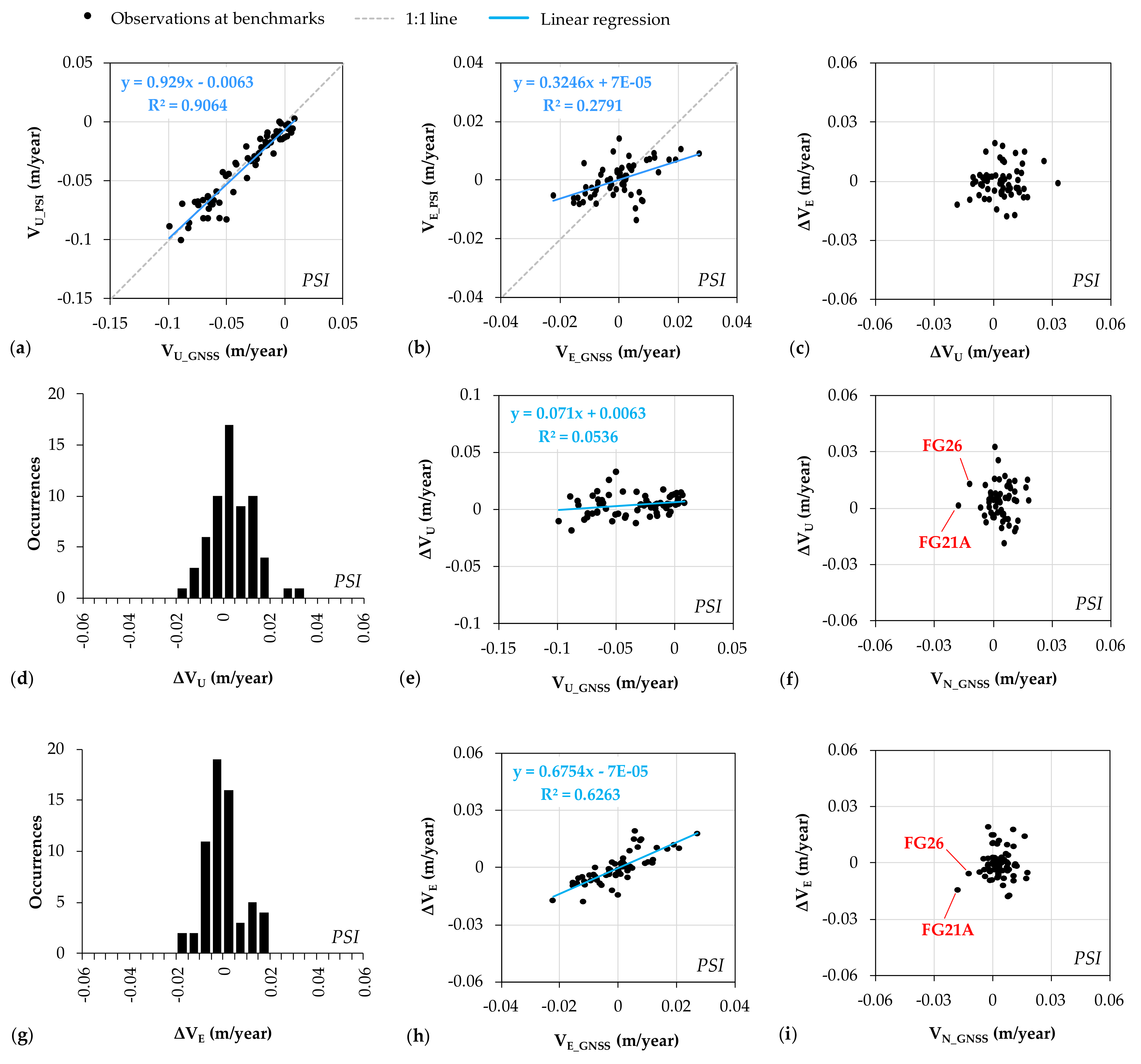
Figure 14.
Comparison of the displacement velocity along the (a) vertical VU and (b) east-west VE direction as estimated from the SBAS InSAR analyses and recorded at the permanent GNSS stations and GNSS benchmarks. The observed differences ΔVU and ΔVE are further investigated through (c) inter-comparison, (d,g) analysis of the respective histograms, and (e,f,h,i) their distribution in relation to GNSS records.
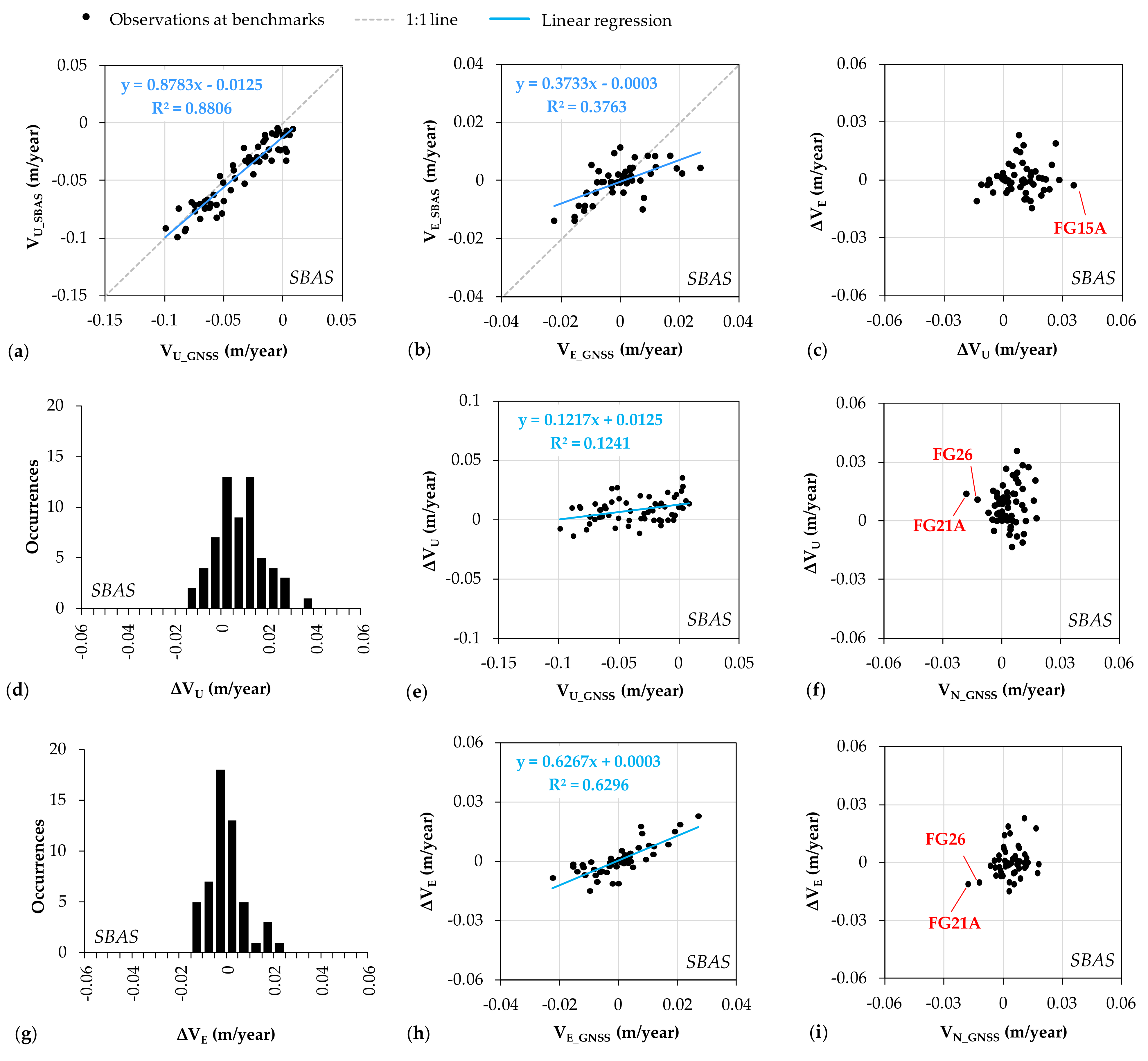
Figure 15.
Estimated magnitude of the contribution to the observed velocity differences (a) ΔVU and (b) ΔVE that is made by the VN = 0 assumption.
Figure 15.
Estimated magnitude of the contribution to the observed velocity differences (a) ΔVU and (b) ΔVE that is made by the VN = 0 assumption.

Figure 16.
Comparison of the displacement velocity along the vertical VU direction as recorded at the geodetic leveling benchmarks and estimated from the InSAR analysis with the (a–c) PSI and (d–f) SBAS methods: (a,d) velocity scatterplots, (b,e) distribution of the observed differences ΔVU, and (c,f) their correlation with the vertical velocity at the leveling benchmarks.
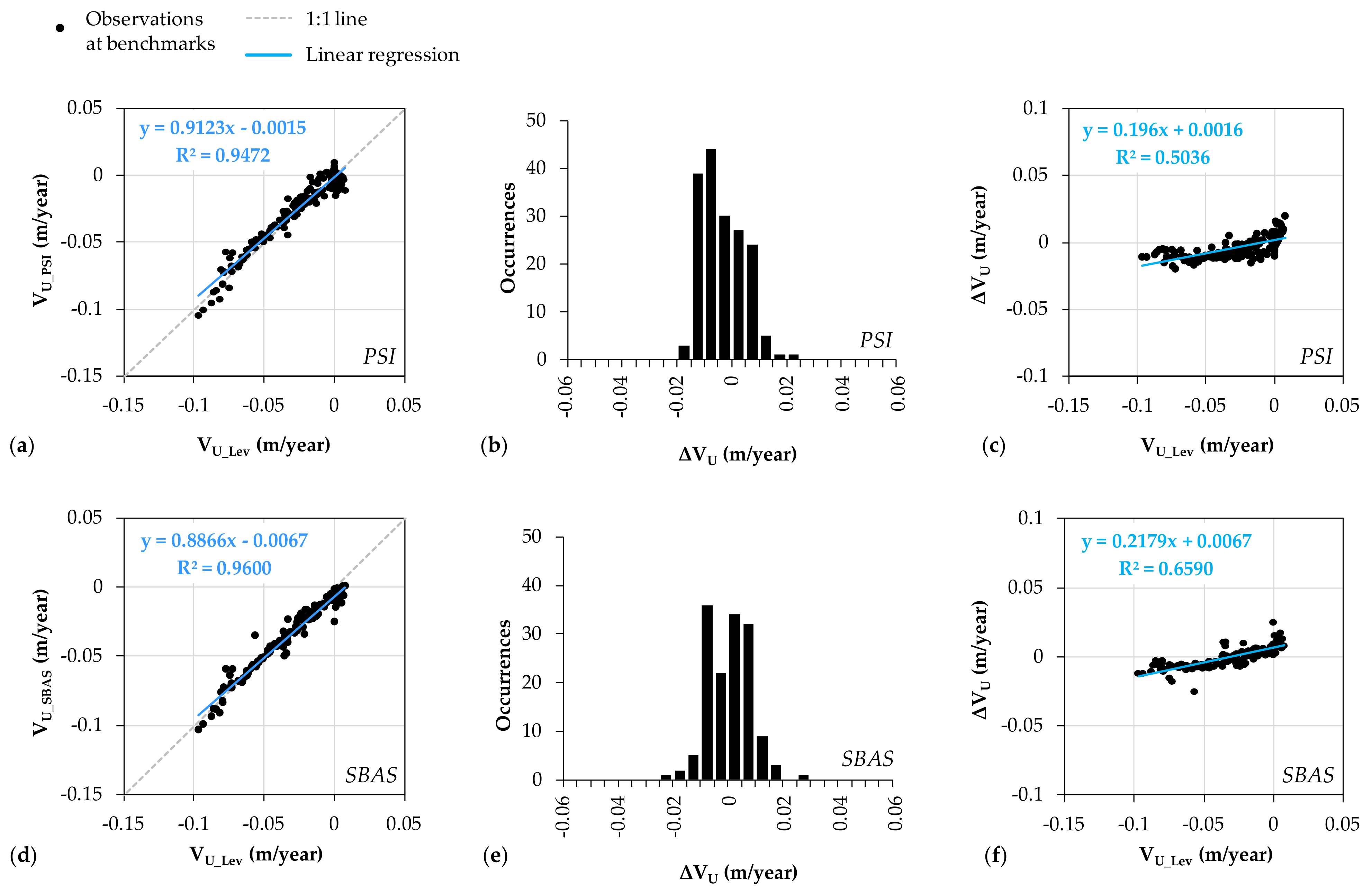
Figure 17.
Location of pairs of monitoring benchmarks F23A−F23B and FG26−FG26A with respect to the Oriente fault trace and grid coverages of SBAS (~90 m blue squares) and PSI up velocities (1 arcsecond pixels, i.e., ~30 m).
Figure 17.
Location of pairs of monitoring benchmarks F23A−F23B and FG26−FG26A with respect to the Oriente fault trace and grid coverages of SBAS (~90 m blue squares) and PSI up velocities (1 arcsecond pixels, i.e., ~30 m).


Table 1.
PSI-SBAS inter-comparison: observed difference in vertical ΔVU and east-west ΔVE velocity estimated from the PSI and SBAS InSAR analyses. The size indicates the number of targets used for comparison, which depends on the coverage of the output datasets. Notation: min., minimum; max., maximum; ave., average; stdv., standard deviation; RMSE, root mean square error.
| Sample | SBAS vs. PSI ΔVU (m/Year) | SBAS vs. PSI ΔVE (m/Year) | ||||||||||
|---|---|---|---|---|---|---|---|---|---|---|---|---|
| Size | Min. | Max. | Ave. | Stdv. | RMSE | Size | Min. | Max. | Ave. | Stdv. | RMSE | |
| GNSS benchmarks | 59 | −0.0289 | +0.0148 | −0.0039 | 0.0060 | 0.0071 | 53 | −0.0147 | +0.0111 | −0.0012 | 0.0042 | 0.0043 |
| All targets | 128,772 | −0.0425 | +0.0555 | −0.0003 | 0.0062 | 0.0063 | 75,546 | −0.0471 | +0.0298 | −0.0004 | 0.0039 | 0.0039 |
Table 2.
Difference in vertical velocity ΔVU estimated from the PSI and SBAS InSAR analyses with respect to that recorded with GNSS (permanent stations and benchmark surveying) and geodetic leveling. The size indicates the number of benchmarks used for comparison.
Table 2.
Difference in vertical velocity ΔVU estimated from the PSI and SBAS InSAR analyses with respect to that recorded with GNSS (permanent stations and benchmark surveying) and geodetic leveling. The size indicates the number of benchmarks used for comparison.
| InSAR Method | GNSS vs. InSAR ΔVU (m/Year) | Leveling vs. InSAR ΔVU (m/year) | ||||||||||
|---|---|---|---|---|---|---|---|---|---|---|---|---|
| Size | Min. | Max. | Ave. | Stdv. | RMSE | Size | Min. | Max. | Ave. | Stdv. | RMSE | |
| PSI | 62 | −0.0186 | +0.0327 | +0.0039 | 0.0092 | 0.0099 | 172 | −0.0195 | +0.0200 | −0.0034 | 0.0077 | 0.0084 |
| SBAS | 61 | −0.0136 | +0.0355 | +0.0081 | 0.0102 | 0.0130 | 145 | −0.0250 | +0.0251 | +0.0005 | 0.0077 | 0.0077 |
Table 3.
Difference in east-west velocity ΔVE estimated from the PSI and SBAS InSAR analyses with respect to that recorded with GNSS (permanent stations and benchmark surveying). The size indicates the number of benchmarks used for comparison.
Table 3.
Difference in east-west velocity ΔVE estimated from the PSI and SBAS InSAR analyses with respect to that recorded with GNSS (permanent stations and benchmark surveying). The size indicates the number of benchmarks used for comparison.
| InSAR Method | GNSS vs. InSAR ΔVE (m/Year) | |||||
|---|---|---|---|---|---|---|
| Size | Min. | Max. | Ave. | Stdv. | RMSE | |
| PSI | 62 | −0.0177 | +0.0194 | −0.0001 | 0.0080 | 0.0079 |
| SBAS | 53 | −0.0149 | +0.0229 | +0.0002 | 0.0076 | 0.0076 |
Publisher’s Note: MDPI stays neutral with regard to jurisdictional claims in published maps and institutional affiliations. |
© 2021 by the authors. Licensee MDPI, Basel, Switzerland. This article is an open access article distributed under the terms and conditions of the Creative Commons Attribution (CC BY) license (https://creativecommons.org/licenses/by/4.0/).
Share and Cite
MDPI and ACS Style
Cigna, F.; Esquivel Ramírez, R.; Tapete, D. Accuracy of Sentinel-1 PSI and SBAS InSAR Displacement Velocities against GNSS and Geodetic Leveling Monitoring Data. Remote Sens. 2021, 13, 4800. https://doi.org/10.3390/rs13234800
AMA Style
Cigna F, Esquivel Ramírez R, Tapete D. Accuracy of Sentinel-1 PSI and SBAS InSAR Displacement Velocities against GNSS and Geodetic Leveling Monitoring Data. Remote Sensing. 2021; 13(23):4800. https://doi.org/10.3390/rs13234800
Chicago/Turabian StyleCigna, Francesca, Rubén Esquivel Ramírez, and Deodato Tapete. 2021. "Accuracy of Sentinel-1 PSI and SBAS InSAR Displacement Velocities against GNSS and Geodetic Leveling Monitoring Data" Remote Sensing 13, no. 23: 4800. https://doi.org/10.3390/rs13234800
Note that from the first issue of 2016, this journal uses article numbers instead of page numbers. See further details here.