
Spatiotemporal Evolution of Wetland Eco-Hydrological Connectivity in the Poyang Lake Area Based on Long Time-Series Remote Sensing Images

Abstract
:
1. Introduction
2. Materials and Methods
2.1. Study Area and Data
2.1.1. Study Area
2.1.2. Data
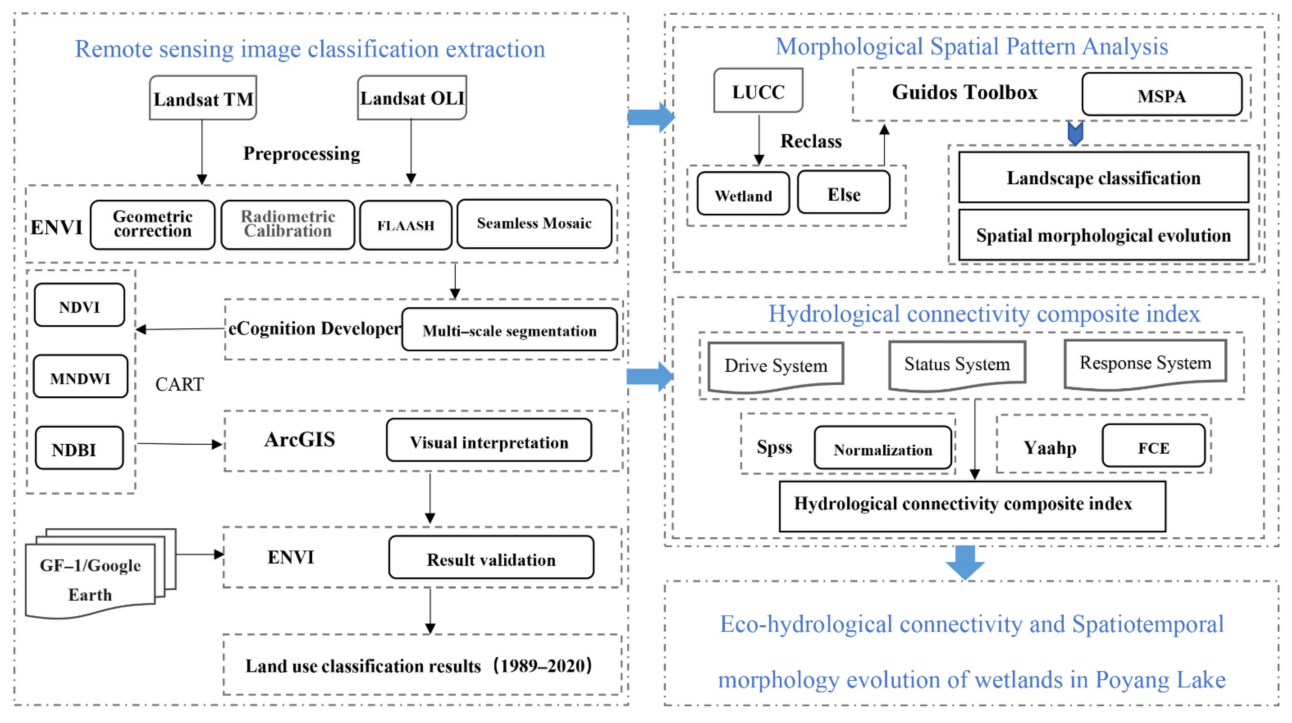
2.2. Methodology
2.2.1. Remote Sensing Image Classification
2.2.2. Landscape Classification Based on the Morphological Spatial Pattern Analysis Model
2.2.3. Hydrological Connectivity Composite Index
VFCmin)
NDVImin)/(VFCmax − VFCmin)
3. Results
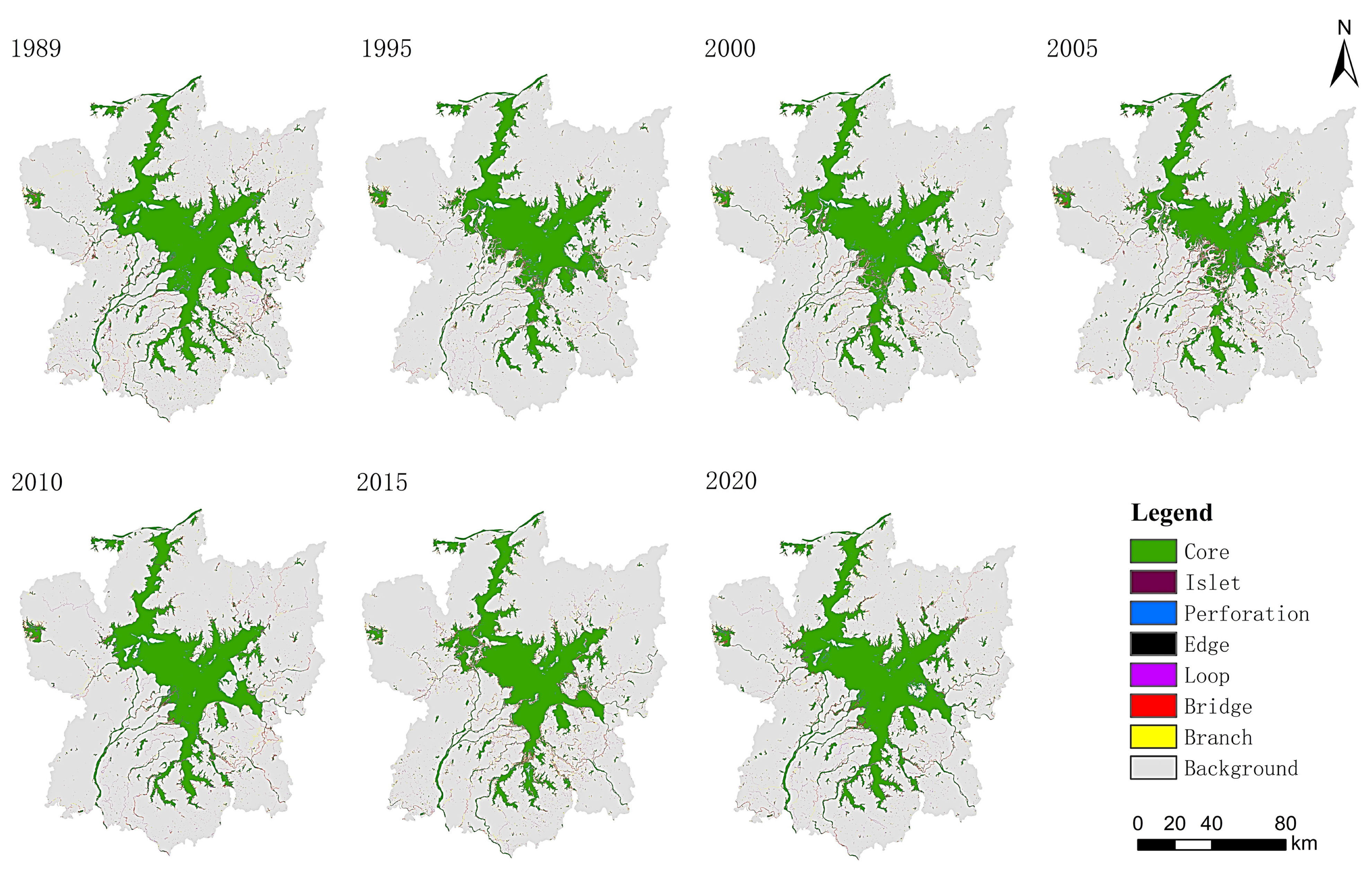
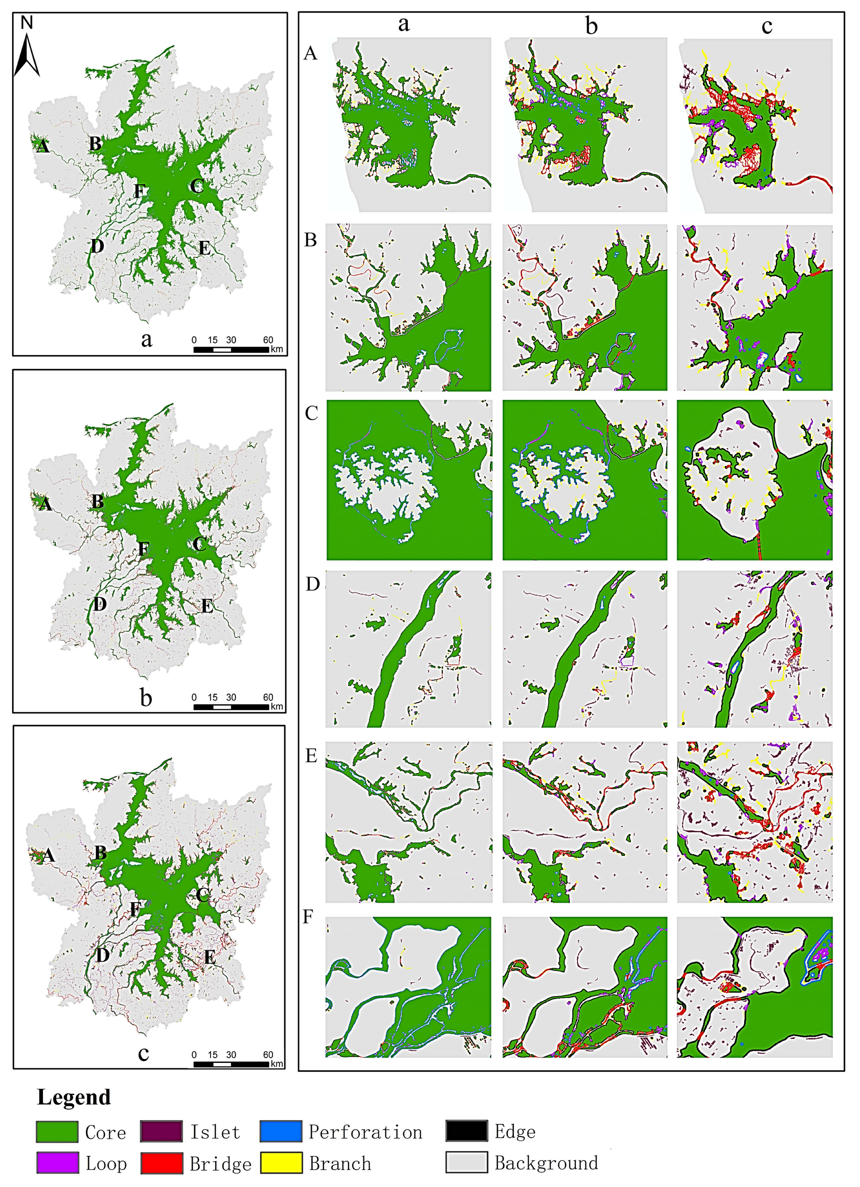
3.1. Landscape Type Changes Based on MSPA from 1989 to 2020
3.1.1. Landscape Type Evolution Characteristics
- (1)
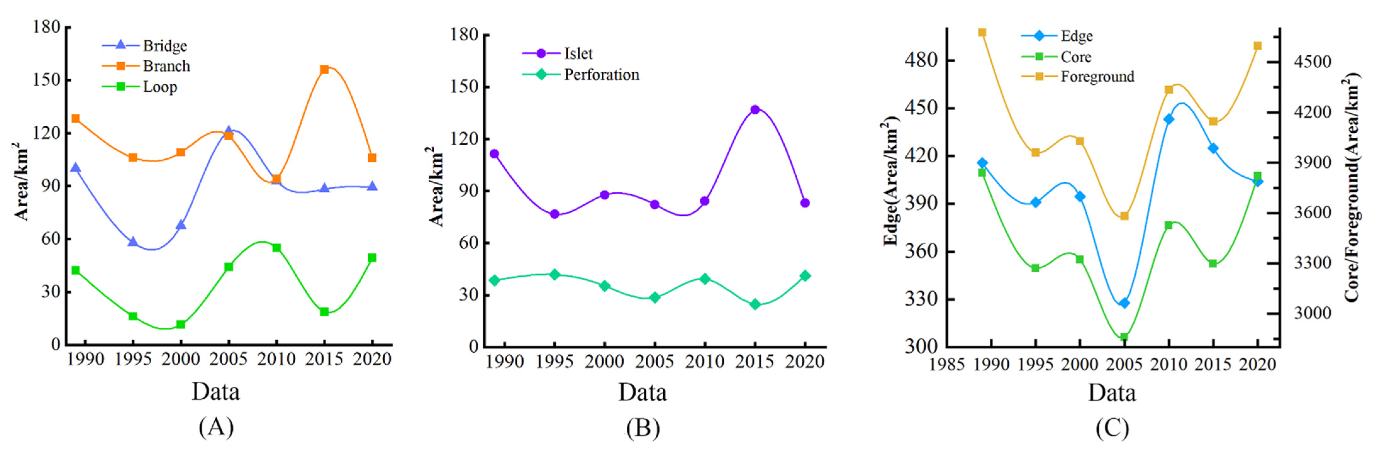
- Core wetlands, edge wetlands, and foregrounds had similar area change trends from 1989 to 2020, all decreasing in the first period and increasing after reaching the lowest point in 2005; the ratio of core areas to foreground areas decreased and then increased from 1989 to 2020. From 1989 to 2005, the wetland landscape was fragmented, and the landscape connectivity decreased, while from 2005 to 2020, the core area increased, and the landscape connectivity was higher. Material and energy exchanges between patches were more frequent, which favored maintaining the stability and biodiversity of wetland ecosystems. Both spatially and in terms of area, the core wetlands exhibited gradual fragmentation followed by recovery from 1989 to 2020 (Figure 5C);
- (2)
- Branches, bridges, and loops all play the role of corridors in the wetland connectivity functions. The contribution of these three types of wetlands to hydrological connectivity was greatest for bridging wetlands, followed by branching wetlands, and least for loop wetlands. The peaks and troughs of bridge and loop wetland areas were practically the same in the period from 1989 to 2020, and both had W-shaped trends, meaning that there were more small rivers in the Poyang Lake area, and they easily disappeared and reappeared due to natural factors. The peak value of branch wetlands appeared in 2015, while the trough value appeared in 2010, with constant fluctuation (Figure 5A);
- (3)
- From 1989 to 2020, the ratio of the islet wetland areas to the foreground wetland areas decreased, then increased, then decreased again. The presence of too many islets increased the number of patches and led to a decrease in the overall connectivity. The area of perforation wetlands was more stable, and was the smallest of the foreground wetlands; the largest was less than 50 km2, and had little impact on the wetland hydrological connectivity (Figure 5B).
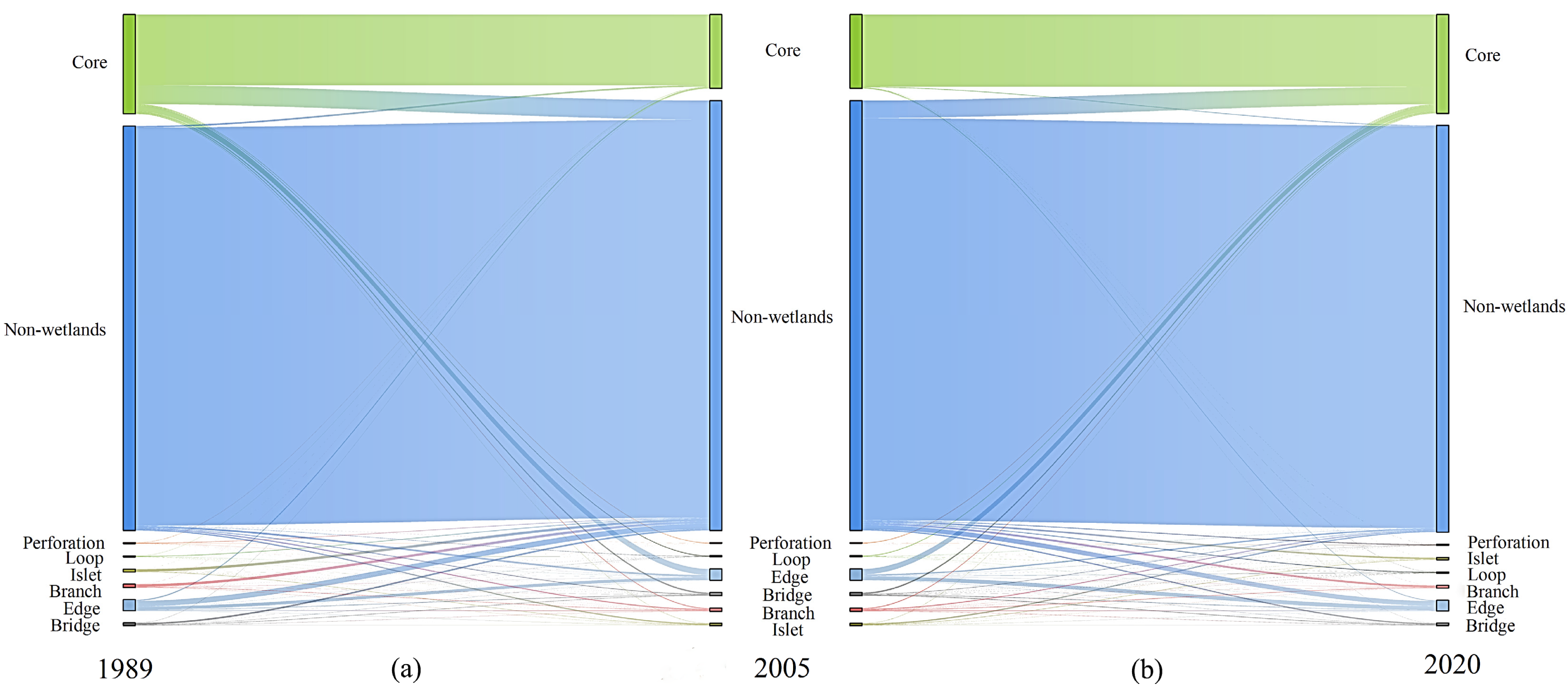
3.1.2. Landscape Type Conversion Characteristics
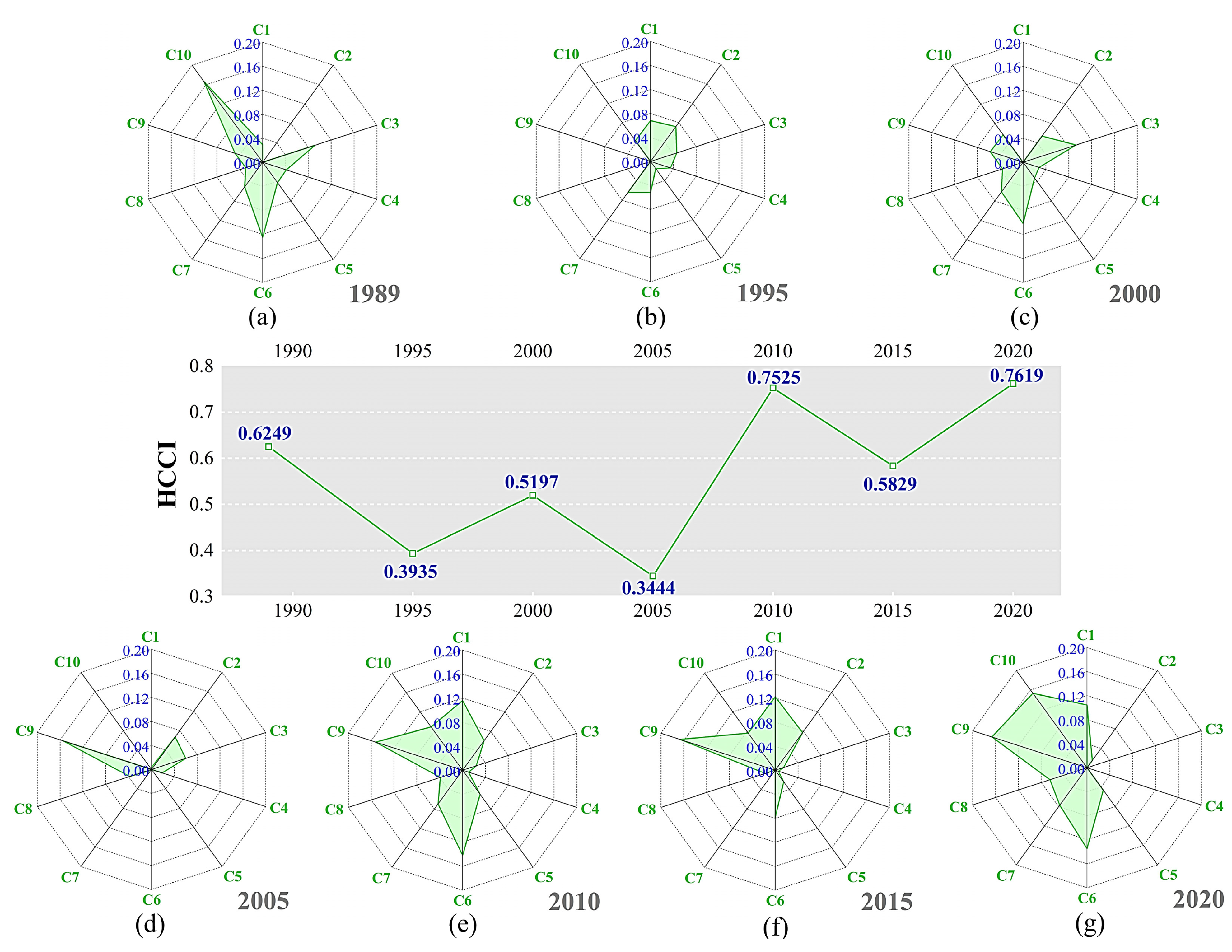
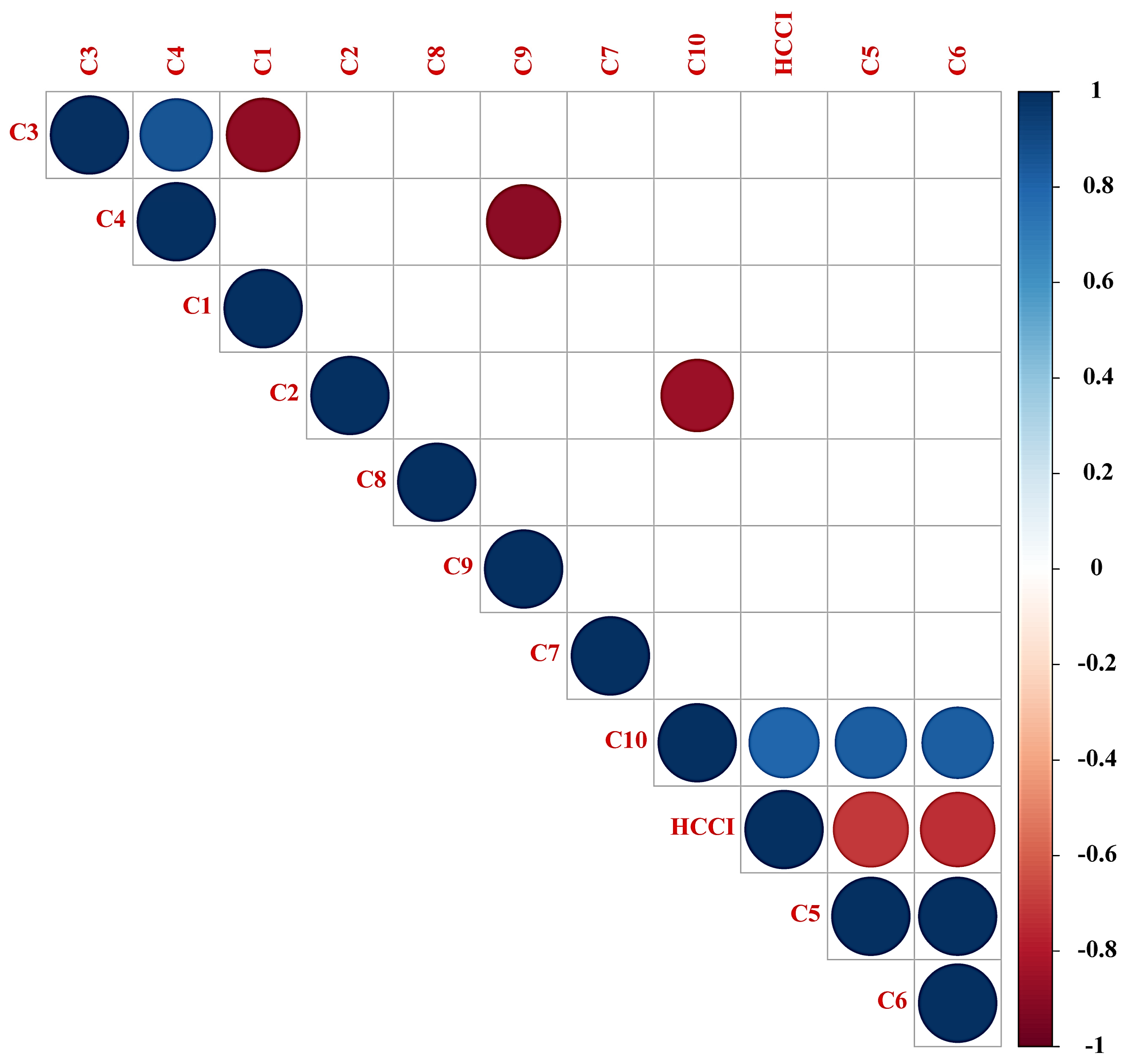
3.2. Evolution of Hydrological Connectivity in the Poyang Lake Area
3.3. Spatial and Temporal Evolution of Hydrological Connectivity: “Receding–Restoring”
4. Discussion
4.1. Influence of Choice of Different Scales on MSPA Results
4.2. Exploring the Drivers of Wetland Hydrological Connectivity
5. Conclusions
Author Contributions
Funding
Institutional Review Board Statement
Informed Consent Statement
Data Availability Statement
Conflicts of Interest
References
- Qu, Y.; Luo, C.; Zhang, H.; Ni, H.; Xu, N. Modeling the wetland restorability based on natural and anthropogenic impacts in Sanjiang Plain, China. Ecol. Indic. 2018, 91, 429–438. [Google Scholar] [CrossRef]
- Liu, X.; Dong, G.; Wang, X.; Xue, Z.; Jiang, M.; Lu, X.; Zhang, Y. Characterizing the spatial pattern of marshlands in the Sanjiang Plain, Northeast China. Ecol. Eng. 2013, 53, 335–342. [Google Scholar] [CrossRef]
- Bracken, L.J.; Croke, J. The concept of hydrological connectivity and its contribution to understanding runoff-dominated geo-morphic systems. Hydrol. Process. 2007, 21, 1749–1763. [Google Scholar] [CrossRef]
- Pringle, C. What Is Hydrologic Connectivity and Why Is It Ecologically Important? Hydrol. Process. 2003, 17, 2685–2689. [Google Scholar] [CrossRef]
- Ward, J.V. The Four-Dimensional Nature of Lotic Ecosystems. J. N. Am. Benthol. Soc. 1989, 8, 2–8. [Google Scholar] [CrossRef]
- Tan, Z.; Li, Y.; Zhang, Q.; Liu, X.; Song, Y.; Xue, C.; Lu, J. Assessing effective hydrological connectivity for floodplains with a framework integrating habitat suitability and sediment suspension behavior. Water Res. 2021, 201, 117253. [Google Scholar] [CrossRef] [PubMed]
- Cohen, M.J.; Creed, I.F.; Alexander, L.; Basu, N.B.; Walls, S.C. Do geographically isolated wetlands influence landscape functions? Proc. Natl. Acad. Sci. USA 2016, 113, 1978–1986. [Google Scholar] [CrossRef] [PubMed] [Green Version]
- Reckendorfer, W.; Funk, A.; Gschpf, C.; Hein, T.; Schiemer, F. Aquatic ecosystem functions of an isolated floodplain and their implications for flood retention and management. J. Appl. Ecol. 2013, 50, 119–128. [Google Scholar] [CrossRef]
- Singh, M.; Sinha, R. Evaluating dynamic hydrological connectivity of a floodplain wetland in North Bihar, India using geostatistical methods. Sci. Total Environ. 2019, 651, 2473–2488. [Google Scholar] [CrossRef]
- Gardner, R.C.; Barchiesi, S.; Beltrame, C.; Finlayson, C.; Galewski, T.; Harrison, I.; Paganini, M.; Perennou, C.; Pritchard, D.; Rosenqvist, A. State of the World’s Wetlands and Their Services to People: A Compilation of Recent Analyses. Soc. Sci. Electron. Publ. 2015, 158, 348–361. [Google Scholar] [CrossRef] [Green Version]
- Wang, J.; Sheng, Y.; Tong, T. Monitoring decadal lake dynamics across the Yangtze Basin downstream of Three Gorges Dam. Remote Sens. Environ. 2014, 152, 251–269. [Google Scholar] [CrossRef]
- Zhao, L.; Liu, Y.; Luo, Y. Assessing Hydrological Connectivity Mitigated by Reservoirs, Vegetation Cover, and Climate in Yan River Watershed on the Loess Plateau, China: The Network Approach. Water 2020, 12, 1742. [Google Scholar] [CrossRef]
- Xu, X.; Xie, Y.; Qi, K.; Luo, Z.; Wang, X. Detecting the response of bird communities and biodiversity to habitat loss and fragmentation due to urbanization. Sci. Total Environ. 2018, 624, 1561–1576. [Google Scholar] [CrossRef]
- Zhao, R.F.; Zhou, H.R.; Xiao, D.N.; Qian, Y.B.; Zhou, K.F. Changes of wetland landscape pattern in the middle and lower reaches of the Tarim River. Acta Ecol. Sin. 2006, 26, 3470–3478. (In Chinese) [Google Scholar]
- Sun, T.; Lin, W.; Chen, G.; Guo, P.; Ying, Z. Wetland ecosystem health assessment through integrating remote sensing and inventory data with an assessment model for the Hangzhou Bay, China. Sci. Total Environ. 2016, 566, 627–640. [Google Scholar] [CrossRef]
- Bracken, L.J.; Wainwright, J.; Ali, G.A.; Tetzlaff, D.; Smith, M.W.; Reaney, S.M.; Roy, A.G. Concepts of hydrological connectivity: Research approaches, pathways and future agendas. Earth Sci. Rev. 2013, 119, 17–34. [Google Scholar] [CrossRef] [Green Version]
- Li, Y.; Zhang, Q.; Cai, Y.; Tan, Z.; Wu, H.; Liu, X.; Yao, J. Hydrodynamic investigation of surface hydrological connectivity and its effects on the water quality of seasonal lakes: Insights from a complex floodplain setting (Poyang Lake, China). Sci. Total Environ. 2019, 660, 245–259. [Google Scholar] [CrossRef] [PubMed]
- Liu, X.; Zhang, Q.; Li, Y.; Tan, Z.; Werner, A.D. Satellite image-based investigation of the seasonal variations in the hydrological connectivity of a large floodplain (Poyang Lake, China). J. Hydrol. 2020, 585, 124810. [Google Scholar] [CrossRef]
- Hein, T.; Hauer, C.; Schmid, M.; Stöglehner, G.; Stumpp, C.; Ertl, T.; Graf, W.; Habersack, H.; Haidvogl, G.; Hood-Novotny, R.; et al. The coupled socio-ecohydrological evolution of river systems: Towards an integrative perspective of river systems in the 21st century. Sci. Total Environ. 2021, 801, 149619. [Google Scholar] [CrossRef]
- Michalek, A.; Zarnaghsh, A.; Husic, A. Modeling linkages between erosion and connectivity in an urbanizing landscape. Sci. Total Environ. 2021, 764, 144255. [Google Scholar] [CrossRef]
- Zhang, Z.; Furman, A. Soil redox dynamics under dynamic hydrologic regimes—A review. Sci. Total Environ. 2021, 763, 143026. [Google Scholar] [CrossRef]
- Wang, N.; Chu, X.; Zhang, X. Functionalities of surface depressions in runoff routing and hydrologic connectivity modeling. J. Hydrol. 2021, 593, 125870. [Google Scholar] [CrossRef]
- Lehmann, P.; Hinz, C.; Mcgrath, G.; Tromp-Van Meerveld, H.J.; Mcdonnell, J.J. Rainfall threshold for hillslope outflow: An emergent property of flow pathway connectivity. Hydrol. Earth Syst. Sci. 2007, 11, 1047–1063. [Google Scholar] [CrossRef] [Green Version]
- McDonough, O.T.; Lang, M.; Hosen, J.; Palmer, M.A. Surface Hydrologic Connectivity Between Delmarva Bay Wetlands and Nearby Streams Along a Gradient of Agricultural Alteration. Wetlands 2015, 35, 41–53. [Google Scholar] [CrossRef]
- Uden, D.R.; Hellman, M.L.; Angeler, D.G.; Allen, C.R. The role of reserves and anthropogenic habitats for functional connectivity and resilience of ephemeral wetlands. Ecol. Appl. 2014, 24, 1569–1582. [Google Scholar] [CrossRef] [PubMed] [Green Version]
- Vanderhoof, M.K.; Distler, H.E.; Lang, M.W.; Alexander, L.C. The influence of data characteristics on detecting wetland/stream surface-water connections in the Delmarva Peninsula, Maryland and Delaware. Wetl. Ecol. Manag. 2017, 26, 63–86. [Google Scholar] [CrossRef]
- Vanderhoof, M.K.; Alexander, L.C.; Todd, M.J. Temporal and spatial patterns of wetland extent influence variability of surface water connectivity in the Prairie Pothole Region, United States. Landsc. Ecol. 2016, 31, 805–824. [Google Scholar] [CrossRef] [Green Version]
- Brooks, J.R.; Mushet, D.M.; Van De Rhoof, M.K.; Leibowitz, S.G.; Christensen, J.R.; Neff, B.P.; Rosenberry, D.O.; Rugh, W.D.; Alexander, L.C. Estimating Wetland Connectivity to Streams in the Prairie Pothole Region: An Isotopic and Remote Sensing Approach. Water Resour. Res. 2018, 54, 955–977. [Google Scholar] [CrossRef]
- Saura, S.; Estreguil, C.; Mouton, C.; Rodríguez-Freire, M. Network analysis to assess landscape connectivity trends: Application to European forests (1990–2000). Ecol. Indic. 2011, 11, 407–416. [Google Scholar] [CrossRef]
- Pascual-Hortal, L.; Saura, S. Comparison and development of new graph-based landscape connectivity indices: Towards the priorization of habitat patches and corridors for conservation. Landsc. Ecol. 2006, 21, 959–967. [Google Scholar] [CrossRef]
- Mclaughlin, D.L.; Kaplan, D.A.; Cohen, M.J. A significant nexus: Geographically isolated wetlands influence landscape hydrology. Water Resour. Res. 2014, 50, 7153–7166. [Google Scholar] [CrossRef]
- Cavalli, M.; Trevisani, S.; Comiti, F.; Marchi, L. Geomorphometric assessment of spatial sediment connectivity in small Alpine catchments. Geomorphology 2013, 188, 31–41. [Google Scholar] [CrossRef]
- Wickham, J.D.; Riitters, K.H.; Wade, T.G.; Vogt, P. A national assessment of green infrastructure and change for the conterminous United States using morphological image processing. Landsc. Urban Plan. 2010, 94, 186–195. [Google Scholar] [CrossRef]
- Jia, Y.; Tang, L.; Xu, M.; Yang, X. Landscape pattern indices for evaluating urban spatial morphology—A case study of Chinese cities. Ecol. Indic. 2019, 99, 27–37. [Google Scholar] [CrossRef]
- Wang, J.; Xu, C.; Pauleit, S.; Kindler, A.; Banzhaf, E. Spatial patterns of urban green infrastructure for equity: A novel exploration. J. Clean. Prod. 2019, 238, 117858. [Google Scholar] [CrossRef]
- Vogt, P.; Riitters, K. GuidosToolbox: Universal digital image object analysis. Eur. J. Remote Sens. 2017, 50, 352–361. [Google Scholar] [CrossRef]
- Xiao, Z.; Zhang, W.; Hao, L. The evolution of spatial and temporal patterns of Zhengzhou ecological network based on MSPA. Arab. J. Geosci. 2021, 14, 1107. [Google Scholar] [CrossRef]
- Hernando, A.; Velazquez, J.; Valbuena, R.; Legrand, M.; Garcia-Abril, A. Influence of the resolution of forest cover maps in evaluating fragmentation and connectivity to assess habitat conservation status. Ecol. Indic. 2017, 79, 295–302. [Google Scholar] [CrossRef]
- Cheng, L.; Xia, N.; Jiang, P.; Zhong, L.; Pian, Y.; Duan, Y.; Huang, Q.; Li, M. Analysis of farmland fragmentation in China Modernization Demonstration Zone since "Reform and Openness": A case study of South Jiangsu Province. Sci. Rep. 2015, 5, 11797. [Google Scholar] [CrossRef] [Green Version]
- Vogt, P.; Riitters, K.H.; Iwanowski, M.; Estreguil, C.; Kozak, J.; Soille, P. Mapping landscape corridors. Ecol. Indic. 2007, 7, 481–488. [Google Scholar] [CrossRef]
- Rincón, V.; Velázquez, J.; Gutiérrez, J.; Hernando, A.; Khoroshev, A.; Gómez, I.; Herráez, F.; Sánchez, B.; Pablo Luque, J.; García-abril, A.; et al. Proposal of new Natura 2000 network boundaries in Spain based on the value of importance for biodiversity and connectivity analysis for its improvement. Ecol. Indic. 2021, 129, 108024. [Google Scholar] [CrossRef]
- Ghaderpour, E.; Vujadinovic, T.; Hassan, Q.K. Application of the Least-Squares Wavelet software in hydrology: Athabasca River Basin. J. Hydrol. Reg. Stud. 2021, 36, 100847. [Google Scholar] [CrossRef]
- Akoko, G.; Le, T.H.; Gomi, T.; Kato, T. A Review of SWAT Model Application in Africa. Water 2021, 13, 1313. [Google Scholar] [CrossRef]
- Li, Z.; Sun, W.; Chen, H.; Xue, B.; Yu, J.; Tian, Z. Interannual and Seasonal Variations of Hydrological Connectivity in a Large Shallow Wetland of North China Estimated from Landsat 8 Images. Remote Sens. 2021, 13, 1214. [Google Scholar] [CrossRef]
- Wu, Y.; Zhang, Y.; Dai, L.; Xie, L.; Zhao, S.; Liu, Y.; Zhang, Z. Hydrological connectivity improves soil nutrients and root architecture at the soil profile scale in a wetland ecosystem. Sci. Total Environ. 2021, 762, 143162. [Google Scholar] [CrossRef] [PubMed]
- Long, C.M.; Pavelsky, T.M. Remote sensing of suspended sediment concentration and hydrologic connectivity in a complex wetland environment. Remote Sens. Environ. 2013, 129, 197–209. [Google Scholar] [CrossRef] [Green Version]
- Park, E.; Latrubesse, E.M. The hydro-geomorphologic complexity of the lower Amazon River floodplain and hydrological connectivity assessed by remote sensing and field control. Remote Sens. Environ. 2017, 198, 321–332. [Google Scholar] [CrossRef]
- Bian, Z.; Gu, Y.; Zhao, J.; Pan, Y.; Li, Y.; Zeng, C.; Wang, L. Simulation of evapotranspiration based on leaf area index, precipitation and pan evaporation: A case study of Poyang Lake watershed, China. Ecohydrol. Hydrobiol. 2019, 19, 83–92. [Google Scholar] [CrossRef]
- Sun, F.; Ma, R.; Liu, C.; He, B. Comparison of the Hydrological Dynamics of Poyang Lake in the Wet and Dry Seasons. Remote Sens. 2021, 13, 985. [Google Scholar] [CrossRef]
- Le, X. Assessment of Degradration Causes and Development of Protection Strategies for the Poyang Lake Wetlands. In Chinese Water Systems: Volume 3: Poyang Lake Basin; Yue, T., Nixdorf, E., Zhou, C., Xu, B., Zhao, N., Fan, Z., Huang, X., Chen, C., Kolditz, O., Eds.; Springer International Publishing: Cham, Switzerland, 2019; pp. 113–124. [Google Scholar] [CrossRef]
- Xu, J.; Fang, C.; Gao, D.; Zhang, H.; Gao, C.; Xu, Z.; Wang, Y. Optical models for remote sensing of chromophoric dissolved organic matter (CDOM) absorption in Poyang Lake. ISPRS J. Photogramm. Remote Sens. 2018, 142, 124–136. [Google Scholar] [CrossRef]
- Feng, W.; Mariotte, P.; Xu, L.; Buttler, A.; Santonja, M. Seasonal variability of groundwater level effects on the growth of Carex cinerascens in lake wetlands. Ecol. Evol. 2020, 10, 517–526. [Google Scholar] [CrossRef] [Green Version]
- Wang, Y.; Molinos, J.G.; Shi, L.; Zhang, M.; Xu, J. Drivers and Changes of the Poyang Lake Wetland Ecosystem. Wetlands 2019, 39, 35–44. [Google Scholar] [CrossRef]
- Earth Explorer. Available online: https://earthexplorer.usgs.gov/ (accessed on 19 November 2021).
- Geospatial Data Cloud. Available online: https://www.gscloud.cn/search (accessed on 19 November 2021).
- National Meteorological Information Center–China Meteorological Data Network. Available online: http://data.cma.cn/ (accessed on 19 November 2021).
- Soille, P.; Vogt, P. Morphological segmentation of binary patterns. Pattern Recogn. Lett. 2009, 30, 456–459. [Google Scholar] [CrossRef]
- Sandbech, H. International Evaluation; National Environmental Research Institute: Roskilde, Denmark, 2003. [Google Scholar]
- Oliver, M.A.; Webster, R. Kriging: A method of interpolation for geographical information systems. Int. J. Geogr. Inf. Syst. 1990, 4, 313–332. [Google Scholar] [CrossRef]
- Miaomiao, L.I.; Bingfang, W.U.; Changzhen, Y. Estimation of Vegetation Fraction in the Upper Basin of Miyun Reservoir by Remote Sensing. Resour. Sci. 2004, 26, 153–159. (In Chinese) [Google Scholar]
- Zhang, A.; Xia, C.; Lin, J.; Chu, J. Landscape evolution characteristic index and application. Prog. Geogr. 2018, 37, 811–822. (In Chinese) [Google Scholar]
- McGarigal, K.; Compton, B.W.; Plunkett, E.B.; DeLuca, W.; Grand, J.; Ene, E.; Jackson, S.D. A landscape index of ecological integrity to inform landscape conservation. Landsc. Ecol. 2018, 33, 1029–1048. [Google Scholar] [CrossRef] [Green Version]
- Feng, H.; Zou, B.; Tang, Y. Scale- and Region-Dependence in Landscape-PM2.5 Correlation: Implications for Urban Planning. Remote Sens. 2017, 9, 918. [Google Scholar] [CrossRef] [Green Version]
- Cui, L.; Li, G.; Chen, Y.; Li, L. Response of Landscape Evolution to Human Disturbances in the Coastal Wetlands in Northern Jiangsu Province, China. Remote Sens. 2021, 13, 2030. [Google Scholar] [CrossRef]
- Sharp, R.; Chaplin-Kramer, R.; Wood, S.; Guerry, A.; Tallis, H.; Ricketts, T.; Nelson, E.; Ennaanay, D.; Wolny, S.; Olwero, N.; et al. InVEST User’s Guide; The Natural Capital Project: Stanford, CA, USA, 2018. [Google Scholar]
- Wang, Y.M.; Chin, K.S. Fuzzy analytic hierarchy process: A logarithmic fuzzy preference programming methodology. Int. J. Approx. Reason. 2011, 52, 541–553. [Google Scholar] [CrossRef] [Green Version]
- Na, W.; Zhao, Z.C. The comprehensive evaluation method of low-carbon campus based on analytic hierarchy process and weights of entropy. Environ. Dev. Sustain. 2021, 23, 9308–9319. [Google Scholar] [CrossRef]
- Wu, H.Y.; Chen, K.L.; Chen, Z.H.; Chen, Q.H.; Qiu, Y.P.; Wu, J.C.; Zhang, J.F. Evaluation for the ecological quality status of coastal waters in East China Sea using fuzzy integrated assessment method. Mar. Pollut. Bull. 2012, 64, 546–555. [Google Scholar] [CrossRef]
- Luo, D.; Wen, X.; Xu, J.; Zhang, H.; Vongphet, S. Delineation of groundwater potential zones using modified weight standardization method and GIS in arid environments: Case study of Ejina Oasis, Inner Mongolia, China. Arab J. Geosci. 2021, 14, 671. [Google Scholar] [CrossRef]
- Leys, C.; Ley, C.; Klein, O.; Bernard, P.; Licata, L. Detecting outliers: Do not use standard deviation around the mean, use absolute deviation around the median. J. Exp. Soc. Psychol. 2013, 49, 764–766. [Google Scholar] [CrossRef] [Green Version]
- Yuan, K.H.; Bushman, B.J. Combining standardized mean differences using the method of maximum likelihood. Psychometrika 2002, 67, 589–607. [Google Scholar] [CrossRef]
- Hantila, F.I.; Preda, G. Polarization Method for Static Fields. IEEE Trans. Magn. 2000, 36, 672–675. [Google Scholar] [CrossRef]
- Cao, Y.; Meichen, F.U.; Xie, M.; Gao, Y.; Yao, S. Landscape connectivity dynamics of urban green landscape based on morphological spatial pattern analysis(MSPA) and linear spectral mixture model(LSMM) in Shenzhen. Acta Ecol. Sin. 2015, 35, 526–536. [Google Scholar] [CrossRef]
- Ya-Ping, Y.U.; Yin, H.W.; Kong, F.H.; Wang, J.J.; Wen-Bin, X.U. Scale effect of Nanjing urban green infrastructure network pattern and connectivity analysis. Chin. J. Appl. Ecol. 2016, 27, 2119–2127. (In Chinese) [Google Scholar]
- Ostapowicz, K.; Vogt, P.; Riitters, K.H.; Kozak, J.; Estreguil, C. Impact of scale on morphological spatial pattern of forest. Landsc. Ecol. 2008, 23, 1107–1117. [Google Scholar] [CrossRef]
- Zhang, Y.; Shen, W.; Li, M.; Lv, Y. Assessing spatio-temporal changes in forest cover and fragmentation under urban expansion in Nanjing, eastern China, from long-term Landsat observations (1987–2017). Appl. Geogr. 2020, 117, 102190. [Google Scholar] [CrossRef]
- Zhang, M.M.; Wu, X.Q. Hydrological connectivity and spatial morphological evolution of Baiyangdian wetlands in the last 20 years. J. Ecol. 2018, 38, 4205–4213. (In Chinese) [Google Scholar]
- Ouyang, Q.; Liu, W. Study on the characteristics of water level change of Poyang Lake in the past 50 years. Yangtze River Basin Resour. Environ. 2014, 23, 1545–1550. (In Chinese) [Google Scholar]
- Zhang, Q.; Li, L.; Wang, Y.G.; Werner, A.D.; Xin, P.; Jiang, T.; Barry, D.A. Has the Three-Gorges Dam made the Poyang Lake wetlands wetter and drier? Geophys. Res. Lett. 2012, 39, 39. [Google Scholar] [CrossRef] [Green Version]
- Han, X.; Chen, X.; Feng, L. Four decades of winter wetland changes in Poyang Lake based on Landsat observations between 1973 and 2013. Remote Sens. Environ. 2015, 156, 426–437. [Google Scholar] [CrossRef]
- Velastegui-Montoya, A.; Lima, A.D.; Adami, M. Multitemporal Analysis of Deforestation in Response to the Construction of the Tucuruí Dam. ISPRS Int. J. Geo. Inf. 2020, 9, 583. [Google Scholar] [CrossRef]
- Wu, Z.; Liu, T.; Xia, M.; Zeng, T. Sustainable livelihood security in the Poyang Lake Ecological Economic Zone: Identifying spatial-temporal pattern and constraints. Appl. Geogr. 2021, 135, 102553. [Google Scholar] [CrossRef]
- Zhang, Y.; Jia, Q.; Prins, H.H.T.; Cao, L.; de Boer, W.F. Effect of conservation efforts and ecological variables on waterbird population sizes in wetlands of the Yangtze River. Sci. Rep. 2015, 5, 17136. [Google Scholar] [CrossRef] [PubMed] [Green Version]


| Image Acquired Date | Track Number | ||
|---|---|---|---|
| 121/039 | 121/040 | 122/040 | |
| 1989 (TM) | 15071989 | 15071989 | 24091989 |
| 1995 (TM) | 02091995 | 02091995 | 25091995 |
| 2000 (TM) | 10092000 | 15092000 | 18062000 |
| 2005 (TM) | 13092005 | 29092005 | 20092005 |
| 2010 (TM) | 19092010 | 18082010 | 19092010 |
| 2015 (OLI) | 09092015 | 09092015 | 02102015 |
| 2020 (OLI) | 06092020 | 06092020 | 28082020 |
| Type | Features and Description |
|---|---|
| Core | The aggregation of a large number of wetland-like elements with a certain distance from the boundary |
| Islet | A collection of wetland images that are disconnected and aggregated in such small numbers that they cannot be used as cores |
| Perforation | Located inside the core wetland and outside as a “fringe wetland” |
| Bridge | Non-core wetland image sets that connect at least two different core classes and exhibit narrow corridor characteristics |
| Loop | A narrow collection of wetland-like elements that connects a core class and has the characteristics of a corridor |
| Branch | A collection of wetlands that is not a core class area and is connected at only one end to an edge class, bridge class, loop class, or perforation class |
| Edge | Refers to the buffer zone between core classes and non-wetlands |
| System Layer | Guideline Layer | Indicator Layer | Description | Weights |
|---|---|---|---|---|
| Comprehensive index of hydrological connectivity in the Poyang Lake area | Drive system | Average annual precipitation (C1) | Direct water source for wetland systems | 0.122 |
| Vegetation cover (C2) | Affects evaporation of water from wetlands | 0.0775 | ||
| Artificial influence rate (C3) | Characterizes land use changes | 0.0926 | ||
| Population density (C4) | Reflects the degree of interference from human activities | 0.0413 | ||
| Status system | Landscape division index (C5) | Characterizes the degree of plaque separation | 0.0495 | |
| Fragmentation index (C6) | Characterizes the degree of plaque fragmentation | 0.1419 | ||
| Agglomeration index (C7) | Characterizes the degree of plaque aggregation | 0.0771 | ||
| Cohesion index (C8) | Characterizes natural state connectivity | 0.0648 | ||
| Response system | Wetland habitat area ratio (C9) | Characterizes ecological connectivity | 0.1667 | |
| Water area rate (C10) | Characterizes lateral hydraulic connectivity | 0.1667 |
| Type | Core | Islet | Perforation | Edge | Loop | Bridge | Branch | Foreground | |
|---|---|---|---|---|---|---|---|---|---|
| 1989 | Area/km2 | 3840.4485 | 111.3966 | 38.5245 | 415.7019 | 42.2577 | 99.8631 | 128.1933 | 4676.386 |
| Number of patches | 4,267,165 | 123,774 | 42,805 | 461,891 | 46,953 | 110,959 | 142,437 | 5,195,984 | |
| 1995 | Area/km2 | 3271.0707 | 76.6548 | 41.886 | 391.0059 | 16.1847 | 57.9402 | 106.1811 | 3960.923 |
| Number of patches | 3,634,523 | 85,172 | 46,540 | 434,451 | 17,983 | 64,378 | 117,979 | 4,401,026 | |
| 2000 | Area/km2 | 3323.4903 | 87.7392 | 35.2872 | 394.6068 | 11.583 | 67.5144 | 109.2087 | 4029.43 |
| Number of patches | 3,692,767 | 97,488 | 39,208 | 438,452 | 12,870 | 75,016 | 121,343 | 4,477,144 | |
| 2005 | Area/km2 | 2859.9669 | 82.2573 | 28.7424 | 327.8358 | 44.1873 | 120.9573 | 118.4742 | 3582.421 |
| Number of patches | 3,177,741 | 91,397 | 31,936 | 492,379 | 49,097 | 134,397 | 131,638 | 3,980,468 | |
| 2010 | Area/km2 | 3528.0117 | 84.1986 | 39.2841 | 443.1411 | 55.0026 | 92.8287 | 94.0311 | 4336.498 |
| Number of patches | 3,920,013 | 93,554 | 43,649 | 364,262 | 61,114 | 103,143 | 104,479 | 4,818,331 | |
| 2015 | Area/km2 | 3297.7746 | 136.9098 | 24.7374 | 424.9269 | 18.7002 | 88.3071 | 156.0105 | 4147.367 |
| Number of patches | 3,664,194 | 152,122 | 27,486 | 472,141 | 20,778 | 98,119 | 173,345 | 4,608,185 | |
| 2020 | Area/km2 | 3823.5933 | 83.1024 | 41.2146 | 404.0793 | 49.3947 | 89.3385 | 105.9831 | 4596.706 |
| Number of patches | 4,248,437 | 92,336 | 45,794 | 448,977 | 54,883 | 99,265 | 117,759 | 5,107,451 | |
| 2020 | |||||||||
|---|---|---|---|---|---|---|---|---|---|
| Core | Edge | Perforation | Branch | Islet | Loop | Bridge | Non-Wetlands | ||
| 1989 | Core | 3519.2385 | 114.5736 | 13.2012 | 7.0272 | 2.8665 | 14.8239 | 19.5174 | 148.59 |
| Edge | 87.0669 | 128.6316 | 3.6612 | 12.6351 | 4.6035 | 10.5525 | 13.9122 | 154.5966 | |
| Perforation | 17.6175 | 2.5137 | 10.8675 | 0.3249 | 0.045 | 0.9846 | 0.4689 | 5.7024 | |
| Branch | 6.3666 | 9.981 | 0.5292 | 15.9417 | 5.5638 | 2.0016 | 4.6791 | 83.0799 | |
| Islet | 2.4066 | 2.0727 | 0.0801 | 2.4921 | 14.5152 | 0.3879 | 1.1322 | 88.2603 | |
| Loop | 10.7991 | 5.7339 | 1.134 | 1.4436 | 0.8667 | 2.1636 | 1.2213 | 18.8622 | |
| Bridge | 12.0609 | 10.3239 | 0.5436 | 5.3721 | 3.4722 | 1.4508 | 12.8961 | 53.7021 | |
| Non-wetlands | 163.5525 | 129.8268 | 11.1771 | 60.6276 | 51.0921 | 16.9731 | 35.4402 | 15,172.5681 | |
| Landscape Type | Pixel 30 m × 30 m | Pixel 60 m × 60 m | Pixel 120 m × 120 m | |||
|---|---|---|---|---|---|---|
| Area/ha | Percentage of Wetlands (%) | Area/ha | Percentage of Wetlands (%) | Area/ha | Percentage of Wetlands (%) | |
| Core | 413,147.61 | 89.88 | 351,956.88 | 74.91 | 307,913.76 | 65.52 |
| Islet | 1867.23 | 0.41 | 16,064.28 | 3.42 | 27,466.56 | 5.84 |
| Perforation | 5289.48 | 1.15 | 4834.08 | 1.03 | 5495.04 | 1.17 |
| Edge | 29,172.42 | 6.35 | 45,729.72 | 9.73 | 44,619.84 | 9.49 |
| Loop | 1357.92 | 0.30 | 10,293.84 | 2.19 | 19,362.24 | 4.12 |
| Bridge | 2458.71 | 0.53 | 22,296.24 | 4.75 | 38,867.04 | 8.27 |
| Branch | 6377.22 | 1.39 | 18,667.80 | 3.97 | 26,212.32 | 5.58 |
| Landscape Type | 30 Edge with 30 m | 60 Edge with 60 m | 120 Edge with 120 m | |||
|---|---|---|---|---|---|---|
| Area/ha | Percentage of Wetlands (%) | Area/ha | Percentage of Wetlands (%) | Area/ha | Percentage of Wetlands (%) | |
| Core | 413,147.61 | 89.88 | 382,359.33 | 83.18 | 352,324.26 | 76.65 |
| Islet | 1867.23 | 0.41 | 8310.24 | 1.81 | 21,616.47 | 4.70 |
| Perforation | 5289.48 | 1.15 | 4121.46 | 0.90 | 4488.21 | 0.98 |
| Edge | 29,172.42 | 6.35 | 40,407.93 | 8.79 | 44,728.92 | 9.73 |
| Loop | 1357.92 | 0.30 | 4939.47 | 1.07 | 10,039.05 | 2.18 |
| Bridge | 2458.71 | 0.53 | 8933.85 | 1.94 | 19,186.56 | 4.17 |
| Branch | 6377.22 | 1.39 | 10,598.31 | 2.31 | 15,255.09 | 3.32 |
Publisher’s Note: MDPI stays neutral with regard to jurisdictional claims in published maps and institutional affiliations. |
© 2021 by the authors. Licensee MDPI, Basel, Switzerland. This article is an open access article distributed under the terms and conditions of the Creative Commons Attribution (CC BY) license (https://creativecommons.org/licenses/by/4.0/).
Share and Cite
Xia, Y.; Fang, C.; Lin, H.; Li, H.; Wu, B. Spatiotemporal Evolution of Wetland Eco-Hydrological Connectivity in the Poyang Lake Area Based on Long Time-Series Remote Sensing Images. Remote Sens. 2021, 13, 4812. https://doi.org/10.3390/rs13234812
Xia Y, Fang C, Lin H, Li H, Wu B. Spatiotemporal Evolution of Wetland Eco-Hydrological Connectivity in the Poyang Lake Area Based on Long Time-Series Remote Sensing Images. Remote Sensing. 2021; 13(23):4812. https://doi.org/10.3390/rs13234812
Chicago/Turabian StyleXia, Yang, Chaoyang Fang, Hui Lin, Huizhong Li, and Bobo Wu. 2021. "Spatiotemporal Evolution of Wetland Eco-Hydrological Connectivity in the Poyang Lake Area Based on Long Time-Series Remote Sensing Images" Remote Sensing 13, no. 23: 4812. https://doi.org/10.3390/rs13234812