Abstract
Stem biomass is a fundamental component of the global carbon cycle that is essential for forest productivity estimation. Over the last few decades, Light Detection and Ranging (LiDAR) has proven to be a useful tool for accurate carbon stock and biomass estimation in various biomes. The aim of this study was to investigate the potential of multispectral LiDAR data for the reliable estimation of single-tree total and barkless stem biomass (TSB and BSB) in an uneven-aged structured forest with complex topography. Destructive and non-destructive field measurements were collected for a total of 67 dominant and co-dominant Abies borisii-regis trees located in a mountainous area in Greece. Subsequently, two allometric equations were constructed to enrich the reference data with non-destructively sampled trees. Five different regression algorithms were tested for single-tree BSB and TSB estimation using height (height percentiles and bicentiles, max and average height) and intensity (skewness, standard deviation and average intensity) LiDAR-derived metrics: Generalized Linear Models (GLMs), Gaussian Process (GP), Random Forest (RF), Support Vector Regression (SVR) and Extreme Gradient Boosting (XGBoost). The results showcased that the RF algorithm provided the best overall predictive performance in both BSB (i.e., RMSE = 175.76 kg and R2 = 0.78) and TSB (i.e., RMSE = 211.16 kg and R2 = 0.65) cases. Our work demonstrates that BSB can be estimated with moderate to high accuracy using all the tested algorithms, contrary to the TSB, where only three algorithms (RF, SVR and GP) can adequately provide accurate TSB predictions due to bark irregularities along the stems. Overall, the multispectral LiDAR data provide accurate stem biomass estimates, the general applicability of which should be further tested in different biomes and ecosystems.
1. Introduction
Stem volume and biomass are among the most significant productivity and carbon sequestration factors since they are vital for sustainable forest management and climate change mitigation [1]. According to [2], plant biomass (above and below ground) is the main conduit for CO2 removal from the atmosphere, storing more than 80% of the total aboveground carbon [3,4].
In recent decades, there has been an increasing demand for accurate and timely vegetation biomass estimation due to the rising consumption of biomass products, especially in managed forests. Above-ground biomass (AGB) is defined as the sum of the dry mass of every tree component standing above the soil level (e.g., stem, leaves, needles, branches, bark), typically expressed as mass at the individual tree level [5,6,7]. Among the different AGB components, the stem biomass is considered to be the most crucial, being the dominant material for timber products and paper production [8]. Traditionally, biomass estimation has been performed through destructive sampling, providing accurate and precise results, yet it is time-consuming, costly and laborious [6,9]. For decades, AGB estimates have mostly been based on allometric models [10], the development of which requires destructive sampling of a significant amount of trees [11] and measurement of their structural parameters, such as diameter at breast height (DBH) and/or tree height [12,13,14]. Depending on the stem biomass allometric equation type, the total stem biomass (TSB) and the barkless stem biomass (BSB) are most frequently estimated, since the TSB is necessary for the AGB and carbon pool estimations, while the BSB is essential for logging productivity estimation. Nowadays, a large number of allometric equations has been established for the vast majority of species in different biomes [15,16,17,18,19], reducing the need for destructive sampling [20]. However, the specific biomass estimation method is rather limited in terms of spatial coverage and the need for equation reconstruction at regular temporal intervals.
Remote sensing technologies provide timely, low-cost, and reliable estimates on biomass and other forest attributes, especially over large and/or remote areas [21]. Optical remote sensing data, such as aerial photography [22,23,24,25,26], multispectral satellite imagery [27,28,29,30,31,32,33], synthetic aperture radar (SAR) [34,35,36,37,38,39], light detection and ranging (respectively) [40,41,42,43,44,45,46,47] and multisource approaches [48,49,50,51,52,53], have been widely used for forest biomass and carbon quantification. Multispectral image analysis is the most common approach for large-scale biomass estimation [21], although the main limitation is the signal saturation over forested areas with high AGB values [54]. SAR systems have been successfully applied in biomass estimation, due to their canopy penetration capabilities which depend on the wavelength and the canopy characteristics [55]. However, SAR data also present significant limitations, including saturation, high cost, and complex processing methods, especially over forested areas with complex topography [56]. On the contrary, Light Detection and Ranging (LiDAR) data usually offer more accurate forest biomass estimates [57], due to the ability of the emitted pulses to penetrate the forest canopy and, therefore, provide 3D information about all forest vegetation layers [58].
Several studies have shown that LiDAR data provide accurate and efficient biomass estimates using either plot- or tree-level approaches. The first approach has been examined in different biomes [9,42,44,59,60,61,62] and includes the implementation of height percentiles and other LiDAR-derived metrics in order to predict forest characteristics at the plot or stand level. However, modeling biomass and forest characteristics using the plot level approach requires a sufficient amount of field plot measurements in order to establish the relationship between the LiDAR-derived features and the reference data [63].
On the contrary, the tree-level approach requires high pulse densities [64] and is primarily based on single-tree segmentation, aiming to derive height and intensity metrics for each individual tree [65]. The effectiveness of this approach is closely related to the accuracy of tree detection and tree crown delineation, which highly depends on the point cloud density and forest structure [66]. Several algorithms have been proposed for accurate crown segmentation and evaluated in different forest ecosystems [59,65,67,68,69], utilizing both point clouds and canopy height models (CHMs). According to [70], tree crown delineation over broadleaved forests resulted in lower detection rates than the conifers, due to the complex shape and crown structure. Nevertheless, the specific approach provides reliable biomass estimates in mixed stands using species-specific models [71] and valuable information for forest management purposes, while requiring a lower amount of field work compared to the plot-based method [72]. Although the plot-level approach is the most widely used approach, tree-level AGB estimation is becoming increasingly popular due to the development of small-footprint and UAV-based LiDAR systems that are capable of providing high-density 3D point clouds.
Regardless of the estimation approach, various regression methods have been applied along with LiDAR data for forest biomass estimation, such as Support Vector Regression (SVR) [73], Random Forest (RF) regression [74], cubist regression trees, Linear Mixed-Effects (LME) [44], Gaussian Process (GP) regression [75], nonparametric regression [76] and Artificial Neural Networks (ANNs) [77]. In particular, [44] compared the effectiveness of different machine learning (ML) algorithms for biomass estimation using both single-tree and plot-based approaches on LiDAR-derived point clouds, reporting that SVR produced the most accurate biomass models. In addition, the authors stated that manual crown delineation does not necessarily result in more accurate biomass estimates since the relationship between the accuracy of both crown delineation and biomass estimation is rather complex. In [78], the authors performed a comparative analysis between the tree-level and area-based approach suggesting their combined implementation for reliable AGB estimation in a boreal forest using the nearest neighbor algorithm.
Although BSB is considered to be the most significant parameter for growth models, stem volume, biomass and carbon allocation among tree species [79], most of the LiDAR-based studies focus on the TSB and AGB estimation. Recently, [75] presented a comparison between the potential of multispectral single-photon and linear-mode LiDAR systems in plot-based TSB estimation, using GP regression. The results showcased that the linear mode LiDAR systems outperformed the single-photon systems in terms of Root Mean Square Error (RMSE). In [74], the authors predicted TSB in a boreal forest, using measurements derived from 1476 trees, low-density LiDAR data and two regression algorithms (RF and linear). According to their findings, the estimation accuracy was similar using RF and linear regression in terms of RMSE and the coefficient of determination (R2), although the RF provided more consistent results over the trials [74]. The stem volume and TSB of individual pines were also examined using full-waveform [1] and discrete-return LiDAR data [80]. As reported by [1], the full-waveform-derived metrics do not improve the volume and biomass estimates significantly compared to the discrete data, due to the limitations of single-tree delineation. In [80], the authors employed the crown geometric volume (CGV) method on LiDAR point cloud to estimate the TSB for three different tree density classes. According to the results, the low tree density sites provided the most accurate stem volume estimates (R2 = 0.68) compared to the others (i.e., R2 = 0.62 for the medium and R2 = 0.44 for the dense), since the high tree density leads to large tree segmentation errors.
Recent developments in LiDAR technology have led to commercial multispectral systems, which provide essential information on the vertical distribution of physiological processes [81]. The intensity of multispectral LiDAR channels contains complementary information for improved land cover and species classification [82,83,84,85]. Until now, the intensity features have been most widely used for land cover and species classification but few studies have examined their contribution to forest inventory parameters and biomass estimation [75,86]. More specifically, [86] compared the capability of multispectral and conventional LiDAR data for modelling and predicting forest characteristics (e.g., AGB, Ginis coefficient of DBHs, Shannon diversity index, and number of trees per hectare) at the plot level in a boreal forest. The results showcased that the multispectral data improved the AGB estimations (i.e., R2 = 0.87 for the multispectral and R2 = 0.72 for the single spectral). In 2020, [87] compared the suitability of monospectral and multispectral LiDAR for canopy fuel parameter estimations in a boreal forest. According to their findings, the multispectral LiDAR provided improved canopy fuel estimates compared to the monospectral LiDAR. Additionally, multispectral LiDAR data are more capable for individual tree detection compared to the monospectral data due to the spectral differentiation of the vegetation objects [88].
Although many different tree species have been examined in the literature, few studies have explored the potential of multispectral LiDAR remote sensing in biomass estimation of the different Abies species [89,90,91], and there are still no studies related to the biomass estimation of the Abies borisii-regis. Furthermore, compared to the vast majority of studies on the biomass estimation in plantations and semi-natural regenerated forests, only a handful of studies have been conducted in uneven-aged structured forests [12,92,93,94,95,96]. In order to fill this literature gap, the present study aims to estimate TSB and BSB in an uneven-aged structured Abies borisii-regis forest employing multispectral LiDAR-derived predictive models. More specifically, two allometric equations were built to derive TSB and BSB estimates, respectively, which were used as additional reference data. Next, a set of regression algorithms (i.e., Generalized Linear Models-GLMs, GP, RF, SVR and Extreme Gradient Boosting—XGBoost) was examined using LiDAR-derived height and pulse intensity information in order to investigate their potential in reliable TSB and BSB estimation.
2. Study Area and Dataset Description
2.1. Study Area
The study was conducted in Pertouli University Forest, located on the southeast side of Mount Pindos in Thessaly, Greece (latitude 39°32′–39°35′N, longitude 21°33′–21°38′E) (Figure 1). The forest has been under the management of the Aristotle University of Thessaloniki since 1934 for research and education purposes. It covers almost 33 km2, and the altitude ranges between 900 and 2050 m, with an average of 1350 m. The climate is characterized as transitional Mediterranean/Mid-European with high variability among seasons. Uneven distribution of the annual precipitation is observed, ranging from 1213.9 mm of rainfall and 328.2 mm of snow in winters to 298.8 mm during the vegetative period. As for the geology, the area’s soil type is classified as Cambisol, and the main rocks are flysch and limestones which, along with the mountainous terrain, are quite vulnerable to weathering and erosion.

Figure 1.
Map of the study area, including the vegetation cover and the road network.
Almost 90% of the forest area is dominated by Abies borisii-regis, and the remaining area is covered by individual trees of Scots pine and black pine (Pinus silvestris and Pinus nigra), beech (Fagus moesiaca), Austrian oak (Quercus cerris), willows (Salix caprea and Salix eleagnos), English yew (Taxus baccata), maple (Acer optusatum), European hop-hornbeam (Ostrya carpinifolia), laburnum (Cytisus laburnum), linden (Tilia cordata) and plantations of foreign species. The forest is divided into 173 management compartments, with a 10-year management rotation, and the selective harvesting approach is applied.
Trees of the genus Abies are tall evergreen conifers of the Pinaceae family, native to high mountain regions in the North Temperate Zone, and Abies borisii-regis is the natural hybrid between Abies alba and Abies cephalonica [97]. Abies borisii-regis composes all-aged stands with many small trees and natural regeneration in the understory and mature trees in the overstory. Τrees of the same age can have different heights, mostly due to biological characteristics, tree to tree competition, and soil quality type.
2.2. Dataset Description
2.2.1. Airborne LiDAR Data
Multispectral LiDAR data were acquired in October 2018 over the Pertouli University Forest, using a RIEGL VQ-1560i-DW laser scanner sensor mounted on an airplane, and included information derived from two spectral channels, namely the Green and Near Infrared (NIR) (532 nm and 1064 nm, respectively). Before their delivery, the preprocessing of the LiDAR data was performed by the provider (i.e., GEOSYSTEMS HELLAS S.A.), including the transformation of the full-waveform dataset (i.e., 19 pulses/m2) to discrete returns. As a result, the delivered data included a georeferenced point cloud in the Universal Transverse Mercator zone 34 coordinates system based on World Geodetic System 1984, along with trajectory files. The point cloud density for both channels was almost identical (i.e., 44.65 points/m2 for the Near Infrared and 44.85 points/m2 for the Green), with identical nominal pulse spacing of 0.15 m and 0.18 m, respectively, up to seven returns per pulse and a scan angle range from −32° to +32°. In addition, aerial photographs were acquired simultaneously with the LiDAR data, providing high resolution images of the entire forest.
2.2.2. Field Survey
Field measurements were conducted in May 2019 and July 2020. The first field survey included non-destructive sampling of tree clusters in six parts of the forest, while during the second survey, destructive sampling of 32 trees was performed in a predetermined forest compartment (Figure 2). We chose to enrich the dataset with non-destructive sampling in order to keep the forest disturbance to a minimum, due to the invasive nature of destructive sampling.

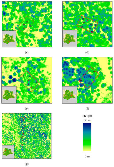
Figure 2.
ALS-generated canopy height model of Pertouli University Forest, showing the sampled trees; (a–f) plots employed for non-destructive sampling (i.e., measurement of DBH for stem biomass estimation using allometric equations); (g) area of interest for destructive sampling.
Non-destructive sampling of stem biomass was carried out in six fixed plots, each of which covered an area of 1000 m2 (40 m × 25 m). The distribution of the sampling plots across the study area was performed according to the different tree density, DBH distribution, and topographic features. This information was derived from the forest census data, of the 10-year forest management plan conducted in 2018. In each plot, only overstory trees that were detectable by the LiDAR sensor were measured. More specifically, DBH was recorded for each selected tree using a Haglof Mantax Blue caliper. Tree locations were determined using a Garmin eTrex 30x touch with an average horizontal position accuracy of 4 m. As a result, a set of 35 non-destructively sampled trees was recorded and correctly identified in the point cloud.
Destructive stem biomass sampling was carried out in one specific forest compartment due to legal restrictions regarding timber harvesting in the study area. As in the previous sampling method, in each plot the measurement was performed only to the trees that could be detected by the LiDAR sensor. The selection of the specific sample trees was based on the different stem diameters, heights and soil qualities with the aim to collect representative samples from all forest conditions. DBH was recorded on the standing trees using a Haglof Mantax Blue caliper, and their locations were determined using a Garmin eTrex 30x touch. Tree height was obtained after the felling of each tree using a Leica Disto D2 laser distance meter and a ruler. In particular, the laser distance meter was used for the measurement of the distance between the top of the tree and the bottom of the trunk, and the ruler was used to measure the length of the above-ground stump portion. The trunk was then separated from the foliage and divided into three different sections according to its shape (neiloid, cone, and paraboloid) [98,99]. A disk sample was taken from each section and the distance between the disks was measured. Likewise, the fresh weight of the disks was measured using a handheld scale. For smaller trees, with a height lower than 10 m, two samples were taken due to the invariable shape of the trunk.
The bark from each sample was removed and stored in separate paper bags. The circumference and the width of each disk without the bark were measured using a tape measure and converted to diameter under the assumption that the tree’s stem is circular [100]. The separated bark samples and the wood were dried at 85 °C for at least 72 h and weighed [98]. The ratio of the measured dry to fresh mass of the stem particles represents the tree wood and bark density. Next, the stem volume was calculated using the following functions (Equations (1)–(3)) [101]:
where H is the distance between the two disks, r1, r2, and r3 are the radius of the first, second, and third disk, respectively, and rs is the radius at the end of the merchantable height. Eventually, the wood and bark density of the samples was multiplied with the volume of each stem partition for the TSB and BSB biomass calculation (Table 1 and Figure 3).

Table 1.
Single-tree biomass metrics based on destructive sampling.
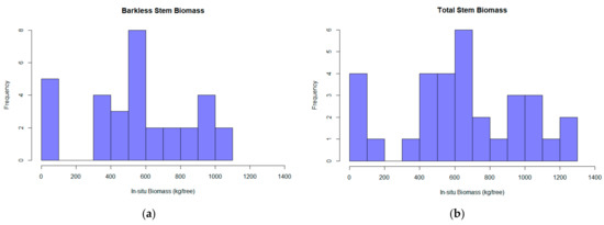
Figure 3.
The barkless stem biomass (BSB) (a) and the total stem biomass (TSB) (b) calculated for each tree based on the destructive sampling implementation.
3. Methods
The methodology for the LiDAR-based TSB and BSB estimation is composed of three separate parts, namely the LiDAR processing, the allometric equations development and the model construction along with its’ cross-validation. Figure 4 illustrates the flowchart of the entire workflow, which is described in detail in the following sections (Section 3.1, Section 3.2 and Section 3.3).
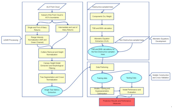
Figure 4.
Workflow of the barkless and total stem biomass (BSB and TSB, respectively) estimation using destructive sampling and ALS data in an uneven-aged structured coniferous forest.
3.1. LiDAR Data Processing
LiDAR data processing was performed using the free and open-source R [102] and Spyder software [103]. First, the collected GPS points from the trees’ positions were buffered to 4 m radius, which represents the radius of the GPS error. This buffered area was used for the identification of the exact field-measured tree within the LiDAR point cloud. Considering that large scan angles can have a significant impact on the LiDAR-derived canopy structure metrics [104] and intensity values are highly affected by the large scan angles [105], echoes with scan angles greater than ±15° were removed to avoid errors originating from off-nadir angles.
Subsequently, range intensity normalization of the point cloud was performed. Since single and first-of-many returns are located higher in the canopy and they are significantly stronger than the intermediate returns, the differences in intensity values are influenced by the large variety of the vegetation materials (i.e., foliage and wood) intercepting with the pulse [106,107]. Furthermore, intensity differences between intermediate and last returns are highly affected by the pulse energy losses sustained at the previous returns and by the pulse discretization procedure [107]. However, it is valid to assume that single and first-of-many returns have no significant transmission loss before being reflected back to the sensor [108]. Therefore, only the single and first-of-many returns were used for the range intensity normalization process, where both incidence angle and target reflectance were considered as constants [9,107,109]. The range normalized intensity (Inorm) was calculated as according to the following equation (Equation (4)):
where is the observed intensity, is the LiDAR-to-object range, is a reference range and the exponent f represents the rate of energy losses by the pulse due to the travel to and from the target [110]. The reference range parameter was set to the average flight altitude and the parameter f was set according to the radar theory [111,112] as f = 2 for targets larger than the footprint [113]. The intensity normalization was performed for each separate flightline and channel (i.e., Green and NIR).
The intensity normalized point cloud was merged with the intermediate and last returns for each tree area and noise removal was performed based on the Statistical Outliers Removal algorithm [114]. The point cloud was classified into ground and non-ground measurements using cloth simulating filtering [115]. Subsequently, the digital terrain model (DTM) was generated, and point cloud height normalization was performed employing the triangulated irregular network (TIN) algorithm. The TIN was preferred over other interpolation algorithms due to its’ effectiveness in areas of steep slopes and densely distributed point clouds [116]. The pit-free algorithm was subsequently employed for CHM generation, since it provides significantly improved tree detection accuracy in high-density LiDAR data [117]. Both the terrain and CHM had a resolution of 0.42 m, which was calculated by the following (5) [118]:
Additionally, morphological erosion with a cross-shaped structuring element was applied to the CHM to reduce the over-segmentation phenomenon of the watershed algorithm [119]. It is also essential to mention that, in this study, the segmentation algorithm was employed without providing treetops or any kind of local maxima feature. Next, single-tree segmentation was performed using the watershed algorithm and the CHM. It is worth noting that a series of established tree segmentation algorithms provided by the package lidR was tested (e.g., [67,69,75]), and the watershed was found to significantly outperform the other algorithms.
Next, a crown normalization process was employed, inspired by the Ptrees algorithm [68], where the correlation between the reference and normalized elevations of each echo is exploited [117]. A simple subtraction of the terrain height from the vegetation points’ height can cause irregularities in the normalized canopy structure in sloped terrains, resulting in a significant impact on the biomass estimation accuracy (Figure 5) [120]. To eliminate the terrain effects to each segmented tree, the highest reference elevation was denoted as the treetop, and the height difference between the treetop’s reference elevation and normalized elevation was calculated. Finally, this height difference was subtracted from the reference height of each echo resulting in the normalized point cloud.
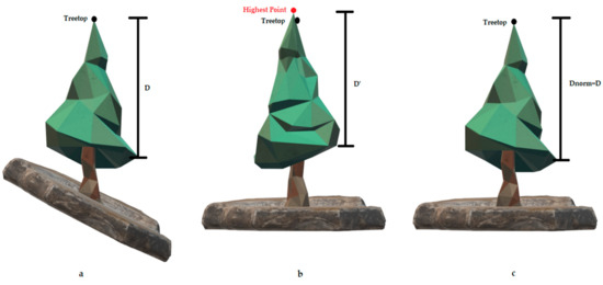
Figure 5.
Effects of the simple DTM-based normalization on the crown structure and the derived parameters. (a) An illustration of the unnormalized tree as it is registered by the LiDAR sensor, where D is the height difference from a specific canopy point to the treetop. (b) The normalized tree using the typical DTM-based normalization procedure, resulting in irregularities in the canopy representation (D > D’) and false detected treetops (red point). (c) The normalized tree using the tree-based normalization procedure, eliminating the effects of the normalization procedure in the canopy structure (Dnorm = D).
In order to confirm that the point cloud of each individual segmented tree actually corresponded to the one measured on the field, we used very-high resolution aerial photographs and field observations, according to the method described in [64]. As a result, all trees measured through destructive sampling and 35 out of 55 tree measurements derived from the non-destructive sampling were successfully identified. Finally, a suite of LiDAR-derived height and intensity metrics were calculated, a summary of which is presented in Table 2.
Table 2.
LiDAR-derived metrics calculated for the stem biomass estimation. All the height metrics were calculated using all the echoes of each point cloud (Green and NIR channels), and the intensity-related metrics were obtained using only first-of-many and single returns.
3.2. Single-Tree Biomass Estimation Using Allometric Equations
As mentioned in the introductory section, stem biomass is usually calculated using the DBH and tree height as inputs in empirical allometric equations. However, no allometric equations are available for stem biomass in Abies borissi-regis. As a result, new species-specific allometric equations were created, using the destructively sampled trees, for total (wood and bark) and woody stem biomass. The most commonly used allometric equation form for biomass estimation is presented below (6):
where a and b are the scaling coefficient and scaling exponent, respectively, y is the estimated biomass and x is a tree dimension variable [121]. The ordinary least squares linear (OLS) regression was used to create two allometric equations based only on DBH. The tree height was not employed so that errors derived by incorrect measurements could be avoided. Such errors can arise since tree height measurement on the field constitutes a rather laborious task, difficult to be performed on standing trees with very high accuracy [122]. Finally, the measured diameters (DBH), TSB and BSB of the 35 non-destructively sampled trees were log-transformed and employed into an OLS regression to determine the scaling coefficients [123]. The performance of the allometric equations was evaluated based on the Relative Square Error (RSE), R2, and Adjusted R2 (adjR2).
3.3. Single-Tree Biomass Estimation Using Regression Algorihtms
In this study, five different regression algorithms, namely Generalized Linear Models (GLMs), Gaussian Process (GP), Random Forest (RF), Support Vector Regression (SVR), and Extreme Gradient Boosting (XGBoost), were examined for their potential to reliably predict both TSB and BSB. Prior to the statistical analysis, all the predictors (i.e., reference data) were “Center” scaled and divided into two sets, namely training (70%) and testing (30%). Additionally, a nested k-fold cross-validation was applied in each training set to obtain the training accuracy of each model, using 10-fold in the outer and 3-fold in the inner loop. The best estimation model was selected based on the arithmetic mean of estimates (i.e., Mean Absolute Error—MAE, Mean Square Error—MSE, relative bias—rbias, RMSE, and R2) in the k-fold cross-validation partitions [77]. The following sections (Section 3.3.1, Section 3.3.2, Section 3.3.3, Section 3.3.4, Section 3.3.5 and Section 3.3.6) present a brief description of each examined algorithm and the respective tuning parameters.
3.3.1. Generalized Linear Models
Introduced by Nelder and Wedderburn [124], generalized linear models provide a wide range of statistical analysis methods [125]. In the present research, a normal error distribution was assumed, and the log link function was employed for the GLM. Furthermore, an exhaustive screening variable selection was applied and a maximum threshold of three variables was defined to avoid overfitting due to the small sample size. During this process, the Small-Sample Corrected Akaike Information Criterion [126] was employed to select the best five models in each fold. Hereafter, the five models were imported to the internal 3-fold cross-validation and the model with the minimum MSE was selected. Last, the best model was selected utilizing the statistics MAE, MSE, and rbias.
3.3.2. Gaussian Process
The GP is a non-parametric technique consisting of a group of random variables, any finite number of which has a joint Gaussian distribution, specified by its mean and covariance function [127]. In regression problems, a Gaussian Process Regression (GPR) model can make predictions utilizing a priori knowledge about similarities between pairs of examples in a domain (kernels) [128] and provide uncertainty measures over predictions [129]. In this study, the radial basis function (rbf) and the linear kernel were tested. As far as the rbf kernel is concerned, a grid search for the sigma inverse width parameter was used, in contrast to the linear kernel, where no hyperparameters were optimized.
3.3.3. Random Forest
Random Forest, introduced by [130], combines several randomized decision trees and ensembles their performance by averaging [131]. According to this approach, a large number of trees are grown from a different bootstrap sample of the data and the predictor variables at each node are randomly selected [132]. In this paper, two hyperparameters were tuned: the number of trees to grow and the number of predictors for each tree. The number of trees to be grown was varied from 50 to 500 with a 50 step, and the number of selected predictors was defined as the number of predictors divided by three [133].
3.3.4. Support Vector Regression
Support Vector Machine (SVM) was initially developed for classification and later extended for regression problems [134]. In regression, the use of a kernel function, the Vapnik–Chervonenkis control of the margin and the number of support vectors are considered as the main characteristics of the SVR [135,136]. The epsilon-SVR algorithm was applied in this study, according to which a nonlinear mapping transforms the input data into an m-dimensional feature space, and a linear model is established [137]. In our work, the rbf kernel was employed and two hyperparameters were optimized, namely the cost of violation of restrictions and sigma parameter.
3.3.5. Extreme Gradient Boosting
The Gradient Boosting algorithm (XGBoost) [138] is an ML technique for regression and classification problems, providing a model in the form of linear combinations of simple predictors by solving an infinite-dimensional convex optimization problem [128,139]. The XGBoost provides a linear model solver and tree learning algorithm based on “boosting decision trees” for regression and classification tasks, preventing over-fitting problems [129]. In this study, the linear-based algorithm was employed, and a set of hyperparameters presented in Table 3 was optimized.
Table 3.
Candidate hyperparameters used for the “XGBoost” algorithm.
3.3.6. Model Performance and Evaluation
The performance of each model was assessed in terms of the MAE, MSE, rbias, R2, and RMSE. The regression models were validated to an independent testing set (i.e., 30% of the total number of samples), which was randomly split from the training data (i.e., 32 destructively and 35 non-destructively in total), to obtain the predictive performance of each algorithm. In addition, the relative importance of individual predictors in each model was evaluated using the variable importance plots [140]. The variance importance, calculated using a model-agnostic procedure [141], provides a list of the ten most significant variables for each model, in descending order. The least important variable could potentially be excluded from the predictive models, decreasing the computational cost [77]. However, in the GLM case, the feature importance represents the percentage of GLMs containing each variable after the training procedure.
4. Results
In the present study, BSB and TSB were estimated using five different regression algorithms. More specifically, allometric equations were initially developed and evaluated for their accuracy to enrich the reference dataset with samples collected by the non-destructive method. Subsequently, five regression algorithms (i.e., GLM, RF, SVR, GP, and XGBoost) were evaluated for their potential in reliably estimating BSB and TSB. In addition, the Pearson’s correlation coefficient was used to evaluate the potentially existing linear association between the LiDAR-derived variables employed in each model (Figure 6) [93]. The results are presented in detail in the following Section 4.2 and Section 4.3.

Figure 6.
Pearson’s correlation matrix between predictor variables derived from multispectral LiDAR data.
4.1. Allometric Equations
Considering that the number of samples (i.e., 32) collected on the field through the destructive sampling method was rather limited, we developed two allometric equations for the BSB and TSB estimation. The development of both models was solely based on the use of DBH without the tree height due to the possible inaccuracy of height measurements. Table 4 presents the results of the allometric TSB and BSB estimation models. The R2 and adjR2 for both models amounted to 0.96; however, the TSB one resulted in higher RSE.
Table 4.
Parameter values, residual standard error, R2 and adjusted R2 for total, and woody stem biomass estimation based on DBH.
4.2. Barkless Stem Biomass
As described in Section 3.3, the BSB of individual trees was predicted using five different regression algorithms (i.e., GLM, RF, SVR, GP, and XGBoost) and the LiDAR-derived intensity and height-related point cloud metrics (Table 2). Table 5 presents the testing performance of the models. The model fits are illustrated in Figure 7, showing the difference between the regression and the hypothetical 1:1 lines.
Table 5.
Average testing performance of the employed algorithms for barkless stem biomass (BSB) estimation using multispectral LiDAR data (i.e., 20 testing samples).
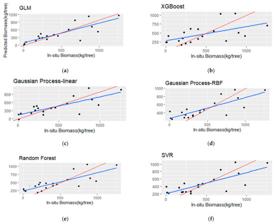
Figure 7.
Scatterplots (a–f) of the observed versus the predicted barkless stem biomass (BSB) for the testing set (i.e., 20 samples). The blue line represents the fitted line, and the red line represents the 1:1 line.
In general, all the models achieved a reasonable prediction with R2 greater than 0.7 and RMSE lower than 195 kg, except for the GP with the linear kernel. More specifically, the developed GLM with three predictors achieved the highest performance in terms of MAE and RMSE, although the highest R2 was obtained by the RF. The RF provided better results compared to the other algorithms (i.e., LR, GP, SVR, XGBoost), with a MAE of 152.65 kg, −5.08% rbias, RMSE of 175.76 kg, and R2 of 0.78. The application of the GP algorithm with the rbf kernel led to the lowest MAE (162.23 kg) and RMSE (184.24 kg), while R2 was higher (i.e., R2 = 0.75) compared to the linear kernel. Both the SVR and the GLM resulted in similar estimation performance, as evidenced by the R2 (0.73 and 0.72, respectively). The XGBoost model gave slightly lower results in terms of R2 (0.69) compared to the RF, GP and GLM algorithms, with the second-highest RMSE (195.25 kg), an MAE of 157.29 kg, and an rbias of −5.08%. Additionally, Table 6 presents the best- and worst-performing linear models, according to the calculated statistical evaluation measures (i.e., MAE, MSE, rbias, RMSE and R2), and the correlation between the variables was examined, showing low correlation (<0.5) between selected predictors (Figure 7).
Table 6.
The best- and worst-performing GLMs selected for the barkless stem biomass (BSB) estimations, using the exhaustive screening variable selection (described in Section 3.3.1).
Regarding the relative predictors’ importance for the BSB estimation (Figure 8), the GP (both examined kernels) and the SVM models indicated the Hmax as the most important variable, followed by the p99, p95 and p90. The same height percentiles were selected by the RF algorithm, which proved to be the best-performing algorithm in terms of R2, followed by the int_std of the NIR channel. The p90 was considered as the most important variable for the XGBoost model as well. On the contrary to the ML algorithms, the int_std of the Green channel was identified as the most important variable presenting the highest frequency of occurrence, alongside the Hmax, p99 and p95 (Table 7). Overall, regarding the ML models, it is evident that the significance of the height-derived LiDAR metrics is considered higher compared to that of the intensity metrics (i.e., int_std_nir), as opposed to the GLM, where the intensity metrics (i.e., int_std_green and int_ske_green) are among the most valuable for the BSB estimation.
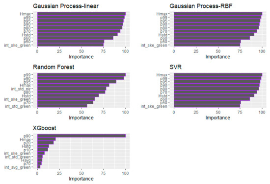
Figure 8.
Demonstration of the relative importance of the predictors for each tested ML algorithm (BSB).
Table 7.
Demonstration of feature importance for the GLM for the barkless stem biomass (BSB) estimation. In this table, the frequency represents the percentage of linear models containing each variable after the testing procedure.
4.3. Total Stem Biomass
The performance of the five different regression algorithms for TSB estimation is presented in this section (Table 8). Additionally, the models’ fit is illustrated in Figure 9, showing a comparison between the regression and the hypothetical 1:1 line. Table 9 presents the best- and worst-performing linear regression models for TSB estimation.
Table 8.
Average testing performance of the employed algorithms for the total stem biomass (TSB) estimation using multispectral LiDAR data (i.e., 20 testing samples).
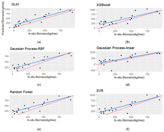
Figure 9.
Scatterplots (a–f) of the observed versus the predicted total stem biomass (TSB) for the testing set (i.e., 20 samples). The blue line represents the fitted line, and the red line represents the 1:1 line.
Table 9.
The best- and worst-performing GLMs selected for the total stem biomass (TSB) estimations, using the exhaustive screening variable selection (described in Section 3.3.1).
The TSB models showed a decrease in R2 and significantly higher RMSE and rbias metrics in comparison with the BSB models. More specifically, the RF model resulted in the highest R2 (0.65) among the other algorithms, but with low MAE (152.65 kg) and RMSE (175.76 kg). The GP with the rbf kernel achieved marginally better R2 over the linear kernel (0.62 and 0.6, respectively), although the latter resulted in lower rbias (−2.02%), RMSE (164.03 kg) and MAE (219.18 kg). The SVR model provided an R2 of 0.57, with a MAE of 166.84 kg and high rbias (−6.15%). The GLM with three predictors achieved low performance in terms of RMSE and R2, although, it showed the lowest rbias (−1.12%). In addition, the best-performing linear model employed high correlated variables (i.e., Havg and p70), which is evidenced in Table 9. Finally, the XGBoost algorithm achieved the lowest R2 (0.31) and the highest RMSE (290.89) compared to the rest of the employed algorithms.
The relative predictor importance of the GLM and ML models for TSB is presented in Table 10 and Figure 10, respectively. In terms of the GLM, the int_std of the Green channel, followed by the p70 and b50 were identified as the most consistent variables for the TSB estimation (Table 10). In all cases, the Hstd was identified as the most important variable. More specifically, in the GP (both examined kernels) and SVR models, the significance of the Hstd was followed by the Hmax. In the RF model case, the Hstd, the p80, and int_ske of both the Green and NIR channels are the four selected most important variables. In the XGBoost model, the Hstd variable was followed by the p80, p30 and int_ske of the NIR channel in terms of importance. It can be observed that, contrary to the BSB model predictors’ importance, the LiDAR-derived intensity metrics from both channels are among the most significant variables, especially in the GLM and the RF model.
Table 10.
Demonstration of feature importance for the GLM for the total stem biomass (TSB) estimation. In this table, the frequency represents the percentage of linear models containing each variable after the testing procedure.
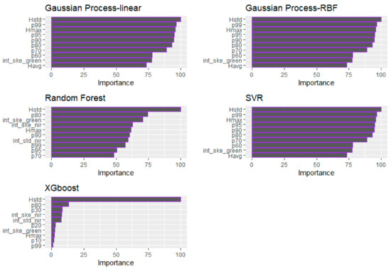
Figure 10.
Demonstration of the relative importance of the predictors employed for each examined algorithm (i.e., RF, SVR, GP, and XGBoost) for the total stem biomass (TSB).
5. Discussion
The present study focuses on the potential of multispectral LiDAR-derived variables alongside with linear and ML regression algorithms for single-tree stem biomass estimation (i.e., TSB and BSB) in an uneven-aged structured forest. In the absence of species-specific allometric equations for biomass estimation, destructive sampling was performed for the construction of two allometric equations (i.e., for TSB and BSB estimation), so that the reference dataset could be enriched without performing additional destructive sampling. Thus, DBH was measured in the field and used as input data in the developed allometric equations for the generation of additional reference TSB and BSB estimates. All reference data were subsequently employed for the tree-level biomass estimation using five different regression algorithms (i.e., GLM, RF, SVR, GP, XGBoost). Both intensity and height metrics were extracted from the LiDAR point cloud and employed as potential independent variables in the predictive models. According to [92], the intensity–height combined AGB models provided higher R2 compared to the ones using only the height information, especially in a study area like the Pertouli University Forest, which is characterized by complex structure, high canopy cover and intense topography [106]. Overall, the results demonstrate that BSB can be reliably estimated using the GLM and the ML algorithms (i.e., RF, SVR, GP and XGBoost) in an uneven-aged structured coniferous forest, while TSB estimations are more reliable using the RF, SVR and GP (with both kernels), with the RF providing the best results in both cases (i.e., BSB and TSB).
In the case of the GLM application, a maximum number of three independent variables (i.e., LiDAR-derived height and intensity metrics) was incorporated in the predictive models in order to avoid potential overfitting. In this study, an exhaustive screening variable selection method and the Small-Sample Corrected Akaike Information Criterion were employed for optimal linear model selection, taking into consideration the MAE, MSE, and rbias statistics. The estimation accuracy of the developed GLM for BSB estimation was similar to the ML models, resulting in the best prediction performance in terms of MAE, MSE, rbias, RMSE and R2 (i.e., MAE = 121.71 kg, MSE = 35585.08 kg, rbias = 1.89%, RMSE = 167.09 kg, R2 = 0.72). However, the GLM severely underperformed (MAE = 174.55 kg, MSE = 45549.33 kg and R2 = 0.44) in the case of the TSB estimation compared to the rest of the examined algorithms (i.e., RF, GP and SVR). Even though the Green channel presents lower sensitivity in canopy returns registration, due to its large beam divergence [142], the int_std was the most frequently selected variable in both BSB and TSB linear models (Table 6 and Table 9). It is noteworthy that the int_std of the Green channel is the variable selected in the best performing linear models, which indicates the significance of the LiDAR intensity information for stem biomass estimation. In general, height metrics were selected in every GLM but, contrary to the intensity metrics, the best performing BSB model consisted of the least frequent height-related variables (i.e., p10 and p70). These two variables are highly correlated, with a Pearson’s correlation coefficient greater than 0.5. Moreover, in the TSB GLM, both the p70 and the b50 were rated as the second and third most frequently selected variables in the best- and worst-performing regression models, respectively (Table 10). A comparison of the BSB and the TSB GLM accuracy reveals that the former performs significantly better. The low predictive performance of the GLM in the TSB estimations can be attributed to the fact that bark volume and biomass variation do not only depend on the tree species but also on the growth rate, the environmental conditions and the genetic constitutions of trees [137]. In addition, allometric equations can introduce uncertainty in the estimated biomass results mainly due to measurement errors, transect size, the fraction of the AGB and the characteristics of the study area [143]. As a result, although the linear models performed well in the BSB predictions, they proved to be inadequate for TSB estimations (i.e., MAE = 173.92 kg, and R2 = 0.32), and new bark biomass ones need to be developed with the use of a large sample size (e.g., sample size >100).
On the contrary, ML algorithms can reliably predict tree attributes in complex structured forests, which is mostly credited to their better generalization ability compared to the GLM [144]. They also provide additional valuable information for the variables, such as the feature importance, which gives the possibility to exclude the insignificant variables with minor contribution to the predictions. However, one of the main limitations of ML algorithms is that they are considered as a black box to users, since it is not feasible to examine the internal iterations and perform detailed interpretations of all model components [74,145].
In the present work, all the ML models had similar performances in the BSB estimations, with the RF presenting the highest values of the statistical evaluation measures (i.e., MAE, RMSE, and R2). As opposed to the GLM, all the ML models identified only height-related LiDAR-derived metrics as the most important features for the prediction of BSB, such as p99, p90, p95, and Hmax. With respect to TSB estimations, the RF algorithm resulted in an R2 of 0.65 with among the lowest MAE and RMSE (i.e., MAE = 152.65 kg and RMSE = 175.76 kg), and identified the Hstd, the p80 and int_ske of both the Green and NIR channels as the most important variables of the regression model. On the contrary, the XGBoost algorithm was found to be prone to overfitting due to the small sample size (i.e., MAE = 236.67 kg, RMSE = 290.89 kg and R2 = 0.31) [146]. According to the literature, the RF algorithm has a significant advantage over the other ML algorithms in terms of its accuracy and its ability to perform with small sample sizes [131]. The RF and GLM-related findings of this work are similar to other studies (e.g., [44,77,146]), although none of them have been conducted in an uneven-aged structured forest.
Although individual tree approaches are becoming increasingly popular due to the rapid development of LiDAR sensors providing high-density point clouds, there is a restricted number of papers for individual tree stem biomass estimation. Consequently, we compared our results with similar reports that exploit either approach, for stem biomass or volume estimation. Despite the complex terrain, the multi-layered forest structure and the denser LiDAR point cloud of [77], we achieved better results in terms of R2 in all of the tested algorithms (i.e., RF, SVR, XGBoost and GLM). In 2020, [147] tested the RF, SVR, and GLM in plantations, resulting in a higher performance compared to ours in terms of R2, but much higher rbias values as well. In addition, [60] used linear models with logarithmic transformations for stem volume estimation in a boreal forest, using primarily height metrics and reported superior results compared to the ones of the present study. This variation in the results can be attributed to the significant difference between the study sites, as the one in our work is a naturally regenerated uneven-aged forest with complex topography, contrary to semi-natural regenerated and hilly forest in Finland.
As for the tree segmentation process, its accuracy was of utmost importance in this study for the subsequent reliable stem biomass estimation since the LiDAR metrics (i.e., potential independent variables for the regression models) are calculated for each individually segmented tree. According to [148], tree segmentation and matching in multi-layered forests is an arduous process resulting in the lowest matching accuracy among the different forest types. More specifically, trees in the lower layers of the forest are difficult to identify and the ability to segment those trees is contextual to the penetration capabilities and pulse characteristics of the LiDAR sensor. Moreover, although multispectral LiDAR sensors provide valuable information on the vertical distribution of physiological processes [81], the higher the degree of canopy overlapping, the lower the capability of tree detection algorithms to accurately identify them [149]. Consequently, only trees able to be detected in the LiDAR point cloud (e.g., dominant, co-dominant) were sampled, aiming to achieve the highest matching rate possible. The destructively sampled trees were all identified in the point cloud, while only 63% of the non-destructively sampled ones were correctly identified. Finally, tree segmentation errors caused by complex forest structure, intense topography, and detection algorithm inaccuracies, could be eliminated by employing a single-tree crown normalization process, based on the watershed segmentation algorithm, and segmenting the point cloud into single trees without prior treetop detection. As a result, the tree height was defined as the highest original point (in the height-unnormalized point cloud), overcoming deformations in the tree crown due to the normalization [120].
Although this research reached its aim, there are some unavoidable limitations. First of all, the sample size is considered small for such a complex structured forest, which has potentially caused additional uncertainty in the predictions [106]. Furthermore, due to legal restrictions, it was not possible to destructively sample a large number of small trees, which could provide better estimates. In addition, this study primarily focused on the trees that could be detected by the LiDAR sensor (e.g., dominant, co-dominant), excluding all the understory trees, which have a significant role in the total forest biomass and dynamics. As a result, the methodology and models can be transferred in similar biomes with the assumption of estimating the stem biomass mainly of the dominant and co-dominant trees. Nevertheless, the segmentation and identification of the understory trees in multi-layered forests with complex terrain is a laborious task due to the overlapping projections of the overstory and the understory tree, which should be studied further.
Overall, the results of our work demonstrated the ability of LiDAR data to estimate individual-tree stem biomass in a multilayered forest, which is critical for forest inventory management and could potentially replace the laborious field measurements required in traditional stem biomass estimation methods. This study also highlights the importance of the pulse intensity metrics in stem biomass estimation, apart from the standard height-derived ones. Besides, this study is the first contribution in the context of LiDAR remote sensing for biomass estimation in an uneven-aged structured Abies borissi-regis forest with complex topography, and one of the few studies that use primarily LiDAR data and destructive sampling for single-tree stem biomass estimation.
6. Conclusions
In this study, we investigated the retrieval of stem biomass estimates at the single-tree level, using multispectral LiDAR data in a complex structured forest. In particular, the BSB and TSB were predicted through linear regression and ML regression algorithms. The results demonstrated the capability of the multispectral LiDAR data to provide reliable stem biomass estimates in a dense, uneven-aged structured forest with rough topography. The main conclusions are listed below:
- BSB can be adequately estimated from all the tested algorithms, contrary to the TSB where only a portion of the selected algorithms (i.e., RF, GP and SVR) provided accurate estimations.
- All the algorithms provided more accurate BSB estimations compared to the TSB ones.
- The RF algorithm resulted in the most precise BSB and TSB estimates in terms of R2 MAE and RMSE, compared to the rest of the examined algorithms.
- The intensity metrics significantly contribute to accurate BSB and TSB estimation, being among the most important variables in the best performing algorithms.
- The ML regression algorithms outperformed the GLM in the TSB estimation, which can be credited to the better generalization capacity and ability of the former to model complex relationships.
It is evident that LiDAR data can significantly contribute to the development and management of complex structured forest resources, providing valuable information about the AGB to different spatial extents. This research aids in improving the stem biomass estimates in uneven-aged structured forests with complex topography, where field measurements can be extremely laborious and costly. The promising results of this study will encourage further research on stem biomass estimation using primarily LiDAR data in complex forests with endemic species, significant for effective forest biomass and carbon management.
Given the limitations of this study described in Section 5, it would be interesting to examine the potential of LiDAR in stem biomass estimation with an increased number of sample trees, in order to validate the results of the present study. In addition, the integration of terrestrial and airborne LiDAR data for stem biomass estimations in complex structured forests could also be investigated, providing additional information about the DBH, tree height and the understory trees. Finally, further research could focus on the contribution of Unmanned Areal Vehicle (UAV) LiDAR systems in tree detection and stem biomass estimation over natural forests.
Author Contributions
Conceptualization, N.G. and I.Z.G.; methodology, N.G., L.K. and I.Z.G.; software, N.G., A.S. and D.S.; validation, N.G. and A.S.; formal analysis, N.G.; investigation, N.G.; resources, I.Z.G.; data curation, N.G.; writing—original draft preparation, N.G.; writing—review and editing, I.Z.G., L.K., A.S. and D.S.; visualization, N.G.; supervision, I.Z.G. and L.K.; project administration, I.Z.G. All authors have read and agreed to the published version of the manuscript.
Funding
Airborne LiDAR data acquisition was funded by the University Forest Administration and Management Fund of the Aristotle University of Thessaloniki (Greece) (http://uniforest.auth.gr/, accessed on 1 November 2021).
Conflicts of Interest
The authors declare no conflict of interest.
References
- Allouis, T.; Durrieu, S.; Vega, C.; Couteron, P. Stem Volume and Above-Ground Biomass Estimation of Individual Pine Trees From LiDAR Data: Contribution of Full-Waveform Signals. IEEE J. Sel. Top. Appl. Earth Obs. Remote Sens. 2013, 6, 924–934. [Google Scholar] [CrossRef]
- Eggleston, S.; Buendia, L.; Miwa, K.; Ngara, T.; Tanabe, K. IPCC Guidelines for National Greenhouse Gas Inventories; IPCC: Geneva, Switzerland, 2006. [Google Scholar]
- Węgiel, A.; Polowy, K. Aboveground Carbon Content and Storage in Mature Scots Pine Stands of Different Densities. Forests 2020, 11, 240. [Google Scholar] [CrossRef] [Green Version]
- Jandl, R.; Lindner, M.; Vesterdal, L.; Bauwens, B.; Baritz, R.; Hagedorn, F.; Johnson, D.W.; Minkkinen, K.; Byrne, K.A. How strongly can forest management influence soil carbon sequestration? Geoderma 2007, 137, 253–268. [Google Scholar] [CrossRef]
- Kajimoto, T.; Matsuura, Y.; Sofronov, M.A.; Volokitina, A.V.; Mori, S.; Osawa, A.; Abaimov, A.P. Above- and belowground biomass and net primary productivity of a Larix gmelinii stand near Tura, central Siberia. Tree Physiol. 1999, 19, 815–822. [Google Scholar] [CrossRef]
- Luo, S.; Wang, C.; Xi, X.; Pan, F.; Peng, D.; Zou, J.; Nie, S.; Qin, H. Fusion of airborne LiDAR data and hyperspectral imagery for aboveground and belowground forest biomass estimation. Ecol. Indic. 2017, 73, 378–387. [Google Scholar] [CrossRef]
- Duncanson, L.; Armston, J.; Disney, M.; Avitabile, V.; Barbier, N.; Calders, K.; Carter, S.; Chave, J.; Herold, M.; MacBean, N.; et al. Aboveground Woody Biomass Product Validation Good Practices Protocol. Land Product Validation Subgroup (Working Group on Calibration and Validation, Committee on Earth Observation Satellites), 2021, 236. Available online: https://lpvs.gsfc.nasa.gov/PDF/CEOS_WGCV_LPV_Biomass_Protocol_2021_V1.0.pdf (accessed on 3 November 2021).
- Zhang, L.; Deng, X.; Lei, X.; Xiang, W.; Peng, C.; Lei, P.; Yan, W. Determining stem biomass of Pinus massoniana L. through variations in basic density. Forestry 2012, 85, 601–609. [Google Scholar] [CrossRef]
- García, M.; Riaño, D.; Chuvieco, E.; Danson, F.M. Estimating biomass carbon stocks for a Mediterranean forest in central Spain using LiDAR height and intensity data. Remote Sens. Environ. 2010, 114, 816–830. [Google Scholar] [CrossRef]
- Dutcă, I.; Zianis, D.; Petrițan, I.C.; Bragă, C.I.; Ștefan, G.; Yuste, J.C.; Petrițan, A.M. Allometric Biomass Models for European Beech and Silver Fir: Testing Approaches to Minimize the Demand for Site-Specific Biomass Observations. Forests 2020, 11, 1136. [Google Scholar] [CrossRef]
- Shearman, T.M.; Varner, J.M.; Robertson, K.; Hiers, J.K. Allometry of the pyrophytic Aristida in fire-maintained longleaf pine–wiregrass ecosystems. Am. J. Bot. 2019, 106, 18–28. [Google Scholar] [CrossRef]
- Xu, Q.; Man, A.; Fredrickson, M.; Hou, Z.; Pitkänen, J.; Wing, B.; Ramirez, C.; Li, B.; Greenberg, J.A. Quantification of uncertainty in aboveground biomass estimates derived from small-footprint airborne LiDAR. Remote Sens. Environ. 2018, 216, 514–528. [Google Scholar] [CrossRef]
- Zianis, D.; Mencuccini, M. On simplifying allometric analyses of forest biomass. For. Ecol. Manag. 2004, 187, 311–332. [Google Scholar] [CrossRef]
- Migolet, P.; Goïta, K.; Ngomanda, A.; Biyogo, A.P.M. Estimation of Aboveground Oil Palm Biomass in a Mature Plantation in the Congo Basin. Forests 2020, 11, 544. [Google Scholar] [CrossRef]
- Djomo, A.N. Allometric equations for biomass estimations in Cameroon and pan moist tropical equations including biomass data from Africa. For. Ecol. Manag. 2010, 260, 1873–1885. [Google Scholar] [CrossRef]
- Chave, J.; Andalo, C.; Brown, S.; Cairns, M.A.; Chambers, J.Q.; Eamus, D.; Fölster, H.; Fromard, F.; Higuchi, N.; Kira, T.; et al. Tree allometry and improved estimation of carbon stocks and balance in tropical forests. Oecologia 2005, 145, 87–99. [Google Scholar] [CrossRef]
- Nogueira, E.M.; Fearnside, P.M.; Nelson, B.W.; Barbosa, R.I.; Keizer, E.W.H. Estimates of forest biomass in the Brazilian Amazon: New allometric equations and adjustments to biomass from wood-volume inventories. For. Ecol. Manag. 2008, 256, 1853–1867. [Google Scholar] [CrossRef]
- Fehrmann, L.; Kleinn, C. General considerations about the use of allometric equations for biomass estimation on the example of Norway spruce in central Europe. For. Ecol. Manag. 2006, 236, 412–421. [Google Scholar] [CrossRef]
- Basuki, T.M.; van Laake, P.E.; Skidmore, A.K.; Hussin, Y.A. Allometric equations for estimating the above-ground biomass in tropical lowland Dipterocarp forests. For. Ecol. Manag. 2009, 257, 1684–1694. [Google Scholar] [CrossRef]
- Martin, F.S.; Navarro-Cerrillo, R.M.; Mulia, R.; van Noordwijk, M. Allometric equations based on a fractal branching model for estimating aboveground biomass of four native tree species in the Philippines. Agrofor. Syst. 2010, 78, 193–202. [Google Scholar] [CrossRef]
- Wang, X.; Jiao, H. Spatial Scaling of Forest Aboveground Biomass Using Multi-Source Remote Sensing Data; IEEE: Piscataway, NJ, USA, 2020. [Google Scholar]
- Ota, T.; Ogawa, M.; Shimizu, K.; Kajisa, T.; Mizoue, N.; Yoshida, S.; Takao, G.; Hirata, Y.; Furuya, N.; Sano, T.; et al. Aboveground Biomass Estimation Using Structure from Motion Approach with Aerial Photographs in a Seasonal Tropical Forest. Forests 2015, 6, 3882–3898. [Google Scholar] [CrossRef] [Green Version]
- Lin, J.; Wang, M.; Ma, M.; Lin, Y. Aboveground Tree Biomass Estimation of Sparse Subalpine Coniferous Forest with UAV Oblique Photography. Remote Sens. 2018, 10, 1849. [Google Scholar] [CrossRef] [Green Version]
- Ota, T.; Ahmed, O.S.; Minn, S.T.; Khai, T.C.; Mizoue, N.; Yoshida, S. Estimating selective logging impacts on aboveground biomass in tropical forests using digital aerial photography obtained before and after a logging event from an unmanned aerial vehicle. For. Ecol. Manag. 2019, 433, 162–169. [Google Scholar] [CrossRef]
- Jannoura, R.; Brinkmann, K.; Uteau, D.; Bruns, C.; Joergensen, R.G. Monitoring of crop biomass using true colour aerial photographs taken from a remote controlled hexacopter. Biosyst. Eng. 2015, 129, 341–351. [Google Scholar] [CrossRef]
- Fensham, R.J.; Fairfax, R.J.; Holman, J.E.; Whitehead, P.J. Quantitative assessment of vegetation structural attributes from aerial photography. Int. J. Remote Sens. 2002, 23, 2293–2317. [Google Scholar] [CrossRef]
- Singh, M.; Malhi, Y.; Bhagwat, S. Biomass estimation of mixed forest landscape using a Fourier transform texture-based approach on very-high-resolution optical satellite imagery. Int. J. Remote Sens. 2014, 35, 3331–3349. [Google Scholar] [CrossRef]
- Muukkonen, P.; Heiskanen, J. Biomass estimation over a large area based on standwise forest inventory data and ASTER and MODIS satellite data: A possibility to verify carbon inventories. Remote Sens. Environ. 2007, 107, 217–624. [Google Scholar] [CrossRef]
- Roy, P.S.; Ravan, S.A. Biomass estimation using satellite remote sensing data—An investigation on possible approaches for natural forest. J. Biosci. 1996, 21, 535–561. [Google Scholar] [CrossRef]
- Sousa, A.M.O.; Gonçalves, A.C.; Mesquita, P.; Marques da Silva, J.R. Biomass estimation with high resolution satellite images: A case study of Quercus rotundifolia. ISPRS J. Photogramm. Remote Sens. 2015, 101, 69–79. [Google Scholar] [CrossRef] [Green Version]
- Muukkonen, P.; Heiskanen, J. Estimating biomass for boreal forests using ASTER satellite data combined with standwise forest inventory data. Remote Sens. Environ. 2005, 99, 434–447. [Google Scholar] [CrossRef]
- Baloloy, A.B.; Blanco, A.C.; Candido, C.G.; Argamosa, R.J.L.; Dumalag, J.B.L.C.; Dimapilis, L.L.C.; Paringit, E.C. Estimation of mangrove forest aboveground biomass using multispectral bands, vegetation indices and biophysical variables derived from optical satellite imageries: Rapideye, Planetscope and sentinel-2. ISPRS Ann. Photogramm. Remote Sens. Spat. Inf. Sci. 2018, IV-3, 29–36. [Google Scholar]
- Steininger, M.K. Satellite estimation of tropical secondary forest above-ground biomass: Data from Brazil and Bolivia. Int. J. Remote Sens. 2000, 21, 1139–1157. [Google Scholar] [CrossRef]
- Schlund, M.; Davidson, M.W.J. Aboveground Forest Biomass Estimation Combining L- and P-Band SAR Acquisitions. Remote Sens. 2018, 210, 1151. [Google Scholar] [CrossRef] [Green Version]
- van Yunjin Kim, J. Zyl Comparison of forest parameter estimation techniques using SAR data. In IGARSS 2001. Scanning the Present and Resolving the Future, Proceedings of the IEEE 2001 International Geoscience and Remote Sensing Symposium (Cat.No.01CH37217), Sydney, Australia, 9–13 July 2001; IEEE: Piscataway, NJ, USA, 2001; Volume 3, pp. 1395–1397. [Google Scholar]
- Solberg, S.; Astrup, R.; Gobakken, T.; Næsset, E.; Weydahl, D.J. Estimating spruce and pine biomass with interferometric X-band SAR. Remote Sens. Environ. 2010, 114, 2353–2360. [Google Scholar] [CrossRef]
- Debastiani, A.B.; Sanquetta, C.R.; Corte, A.P.D.; Rex, F.E.; Pinto, N.S. Evaluating SAR-optical sensor fusion for aboveground biomass estimation in a Brazilian tropical forest. Ann. For. Res. 2019, 62, 109–122. [Google Scholar] [CrossRef]
- Hamdan, O.; Aziz, H.K.; Rahman, K.A. Remotely sensed l-band sar data for tropical forest biomass estimation. J. Trop. For. Sci. 2021, 11, 318–327. [Google Scholar]
- Santoro, M.; Cartus, O. Research Pathways of Forest Above-Ground Biomass Estimation Based on SAR Backscatter and Interferometric SAR Observations. Remote Sens. 2018, 10, 608. [Google Scholar] [CrossRef] [Green Version]
- Kronseder, K.; Ballhorn, U.; Böhm, V.; Siegert, F. Above ground biomass estimation across forest types at different degradation levels in Central Kalimantan using LiDAR data. Int. J. Appl. Earth Obs. Geoinf. 2012, 18, 37–48. [Google Scholar] [CrossRef]
- Drake, J.B.; Knox, R.G.; Dubayah, R.O.; Clark, D.B.; Condit, R.; Blair, J.B.; Hofton, M. Above-ground biomass estimation in closed canopy Neotropical forests using lidar remote sensing: Factors affecting the generality of relationships. Glob. Ecol. 2003, 12, 147–159. [Google Scholar] [CrossRef]
- Ene, L.T.; Næsset, E.; Gobakken, T.; Gregoire, T.G.; Ståhl, G.; Nelson, R. Assessing the accuracy of regional LiDAR-based biomass estimation using a simulation approach. Remote Sens. Environ. 2012, 123, 579–592. [Google Scholar] [CrossRef]
- Popescu, S.C. Estimating biomass of individual pine trees using airborne lidar. Biomass Bioenergy 2007, 31, 646–655. [Google Scholar] [CrossRef]
- Gleason, C.J.; Im, J. Forest biomass estimation from airborne LiDAR data using machine learning approaches. Remote Sens. Environ. 2012, 125, 80–91. [Google Scholar] [CrossRef]
- Popescu, S.C.; Wynne, R.H.; Nelson, R.F. Measuring individual tree crown diameter with lidar and assessing its influence on estimating forest volume and biomass. Can. J. Remote Sens. 2003, 29, 564–577. [Google Scholar] [CrossRef]
- Ståhl, G.; Holm, S.; Gregoire, T.G.; Gobakken, T.; Næsset, E.; Nelson, R. Model-based inference for biomass estimation in a LiDAR sample survey in Hedmark County, NorwayThis article is one of a selection of papers from Extending Forest Inventory and Monitoring over Space and Time. Can. J. For. Res. 2011, 41, 96–107. [Google Scholar] [CrossRef] [Green Version]
- Stovall, A.E.; Vorster, A.G.; Anderson, R.S.; Evangelista, P.H.; Shugart, H.H. Non-destructive aboveground biomass estimation of coniferous trees using terrestrial LiDAR. Remote Sens. Environ. 2017, 200, 31–42. [Google Scholar] [CrossRef]
- Næsset, E.; Gobakken, T.; Solberg, S.; Gregoire, T.G.; Nelson, R.; Ståhl, G.; Weydahl, D. Model-assisted regional forest biomass estimation using LiDAR and InSAR as auxiliary data: A case study from a boreal forest area. Remote Sens. Environ. 2011, 115, 3599–3614. [Google Scholar] [CrossRef]
- Ghosh, S.M.; Behera, M. Aboveground biomass estimation using multi-sensor data synergy and machine learning algorithms in a dense tropical forest. Appl. Geogr. 2018, 96, 29–40. [Google Scholar] [CrossRef]
- Huang, X.; Ziniti, B.; Torbick, N.; Ducey, M.J. Assessment of Forest above Ground Biomass Estimation Using Multi-Temporal C-band Sentinel-1 and Polarimetric L-band PALSAR-2 Data. Remote Sens. 2018, 150, 1424. [Google Scholar] [CrossRef] [Green Version]
- Li, Y.; Li, M.; Li, C.; Liu, Z. Forest aboveground biomass estimation using Landsat 8 and Sentinel-1A data with machine learning algorithms. Sci. Rep. 2020, 10, 9952. [Google Scholar] [CrossRef]
- He, Q.-S.; Cao, C.-X.; Chen, E.-X.; Sun, G.-Q.; Ling, F.-L.; Pang, Y.; Zhang, H.; Ni, W.-J.; Xu, M.; Li, Z.-Y.; et al. Forest stand biomass estimation using ALOS PALSAR data based on LiDAR-derived prior knowledge in the Qilian Mountain, western China. Int. J. Remote Sens. 2011, 33, 710–729. [Google Scholar] [CrossRef]
- Chang, J.; Shoshany, M. Mediterranean shrublands biomass estimation using Sentinel-1 and Sentinel-2. In Proceedings of the 2016 IEEE International Geoscience and Remote Sensing Symposium (IGARSS), Beijing, China, 10–15 July 2016. [Google Scholar]
- Naik, P.; Dalponte, M.; Bruzzone, L. Prediction of Forest Aboveground Biomass Using Multitemporal Multispectral Remote Sensing Data. Remote Sens. 2021, 13, 1282. [Google Scholar] [CrossRef]
- Kaasalainen, S.; Holopainen, M.; Karjalainen, M.; Vastaranta, M.; Kankare, V.; Karila, K.; Osmanoglu, B. Combining Lidar and Synthetic Aperture Radar Data to Estimate Forest Biomass: Status and Prospects. Forests 2015, 6, 252–270. [Google Scholar] [CrossRef]
- Sinha, S.; Jeganathan, C.; Sharma, L.K.; Nathawat, M.S. A review of radar remote sensing for biomass estimation. Int. J. Environ. Sci. Technol. 2015, 142, 1779–1792. [Google Scholar] [CrossRef] [Green Version]
- Laurin, G.V.; Puletti, N.; Grotti, M.; Stereńczak, K.; Modzelewska, A.; Lisiewicz, M.; Sadkowski, R.; Kuberski, Ł.; Chirici, G.; Papale, D. Species dominance and above ground biomass in the Białowieża Forest, Poland, described by airborne hyperspectral and lidar data. Int. J. Appl. Earth Obs. Geoinf. 2020, 92, 102178. [Google Scholar] [CrossRef]
- Jiang, X.; Li, G.; Lu, D.; Chen, E.; Wei, X. Stratification-Based Forest Aboveground Biomass Estimation in a Subtropical Region Using Airborne Lidar Data. Remote Sens. 2020, 12, 1101. [Google Scholar] [CrossRef] [Green Version]
- Silva, C.A.; Saatchi, S.; Garcia, M.; Labriere, N.; Klauberg, C.; Ferraz, A.; Meyer, V.; Jeffery, K.J.; Abernethy, K.; White, L.; et al. Comparison of Small- and Large-Footprint Lidar Characterization of Tropical Forest Aboveground Structure and Biomass: A Case Study From Central Gabon. IEEE J. Sel. Top. Appl. Earth Obs. Remote Sens. 2018, 11, 3512–3526. [Google Scholar] [CrossRef] [Green Version]
- Maltamo, M.; Eerikäinen, K.; Packalén, P.; Hyyppä, J. Estimation of stem volume using laser scanning-based canopy height metrics. For. Int. J. For. Res. 2006, 79, 217–229. [Google Scholar] [CrossRef] [Green Version]
- Næsset, E. Practical large-scale forest stand inventory using a small-footprint airborne scanning laser. Scand. J. For. Res. 2004, 19, 164–179. [Google Scholar] [CrossRef]
- Kelley, J.; Bone, C. Use of Multi-Temporal LiDAR to Quantify Fertilization Effects on Stand Volume and Biomass in Late-Rotation Coastal Douglas-Fir Forests. Forests 2021, 12, 517. [Google Scholar] [CrossRef]
- Yu, X.; Hyyppä, J.; Holopainen, M.; Vastaranta, M. Comparison of Area-Based and Individual Tree-Based Methods for Predicting Plot-Level Forest Attributes. Remote Sens. 2010, 2, 1481–1495. [Google Scholar] [CrossRef] [Green Version]
- Goldbergs, G.; Levick, S.R.; Lawes, M.; Edwards, A. Hierarchical integration of individual tree and area-based approaches for savanna biomass uncertainty estimation from airborne LiDAR. Remote Sens. Environ. 2018, 205, 141–150. [Google Scholar] [CrossRef]
- Latella, M.; Sola, F.; Camporeale, C. A Density-Based Algorithm for the Detection of Individual Trees from LiDAR Data. Remote Sens. 2021, 13, 322. [Google Scholar] [CrossRef]
- Vauhkonen, J.; Ene, L.; Gupta, S.; Heinzel, J.; Holmgren, J.; Pitkanen, J.; Solberg, S.; Wang, Y.; Weinacker, H.; Hauglin, K.M.; et al. Comparative testing of single-tree detection algorithms under different types of forest. Forestry 2012, 85, 27–40. [Google Scholar] [CrossRef] [Green Version]
- Li, W.; Guo, Q.; Jakubowski, M.K.; Kelly, M. A New Method for Segmenting Individual Trees from the Lidar Point Cloud. Photogramm. Eng. Remote Sens. 2012, 78, 75–84. [Google Scholar] [CrossRef] [Green Version]
- Vega, C.; Hamrouni, A.; El Mokhtari, S.; Morel, J.; Bock, J.; Renaud, J.-P.; Bouvier, M.; Durrieu, S. PTrees: A point-based approach to forest tree extraction from lidar data. Int. J. Appl. Earth Obs. Geoinf. 2014, 33, 98–108. [Google Scholar] [CrossRef]
- Silva, C.A.; Hudak, A.T.; Vierling, L.A.; Loudermilk, E.L.; O’Brien, J.J.; Hiers, J.K.; Jack, S.B.; Gonzalez-Benecke, C.; Lee, H.; Falkowski, M.J.; et al. Imputation of Individual Longleaf Pine (Pinus palustris Mill.) Tree Attributes from Field and LiDAR Data. Can. J. Remote Sens. 2016, 42, 554–573. [Google Scholar] [CrossRef]
- Koch, B.; Heyder, U.; Weinacker, H. Detection of individual tree crowns in airborne lidar data. Photogramm. Eng. Remote Sens. 2006, 72, 357–363. [Google Scholar] [CrossRef] [Green Version]
- Yao, W.; Krzystek, P.; Heurich, M. Tree species classification and estimation of stem volume and DBH based on single tree extraction by exploiting airborne full-waveform LiDAR data. Remote Sens. Environ. 2012, 123, 368–380. [Google Scholar] [CrossRef]
- Kaartinen, H.; Hyyppä, J.; Yu, X.; Vastaranta, M.; Hyyppä, H.; Kukko, A.; Holopainen, M.; Heipke, C.; Hirschmugl, M.; Morsdorf, F.; et al. An International Comparison of Individual Tree Detection and Extraction Using Airborne Laser Scanning. Remote Sens. 2012, 4, 950–974. [Google Scholar] [CrossRef] [Green Version]
- De Almeida, C.T.; Galvão, L.S.; Aragão, L.E.d.O.C.E.; Ometto, J.P.H.B.; Jacon, A.D.; Pereira, F.R.d.S.; Sato, L.Y.; Lopes, A.P.; Graça, P.M.L.d.A.; Silva, C.V.d.J.; et al. Combining LiDAR and hyperspectral data for aboveground biomass modeling in the Brazilian Amazon using different regression algorithms. Remote Sens. Environ. 2019, 232, 111323. [Google Scholar] [CrossRef]
- Yu, X.; Hyyppä, J.; Vastaranta, M.; Holopainen, M.; Viitala, R. Predicting individual tree attributes from airborne laser point clouds based on the random forests technique. ISPRS J. Photogramm. Remote Sens. 2011, 66, 28–37. [Google Scholar] [CrossRef]
- Räty, J.; Varvia, P.; Korhonen, L.; Savolainen, P.; Maltamo, M.; Packalen, P. A Comparison of Linear-Mode and Single-Photon Airborne LiDAR in Species-Specific Forest Inventories. IEEE Trans. Geosci. Remote Sens. 2021, 1–14. [Google Scholar] [CrossRef]
- Packalen, P.; Maltamo, M. Predicting the Plot Volume by Tree Species Using Airborne Laser Scanning and Aerial Photographs. For. Sci. 2006, 52, 611–622. [Google Scholar]
- Corte, A.P.D.; Souza, D.V.; Rex, F.E.; Sanquetta, C.R.; Mohan, M.; Silva, C.A.; Zambrano, A.M.A.; Prata, G.; de Almeida, D.R.A.; Trautenmüller, J.W.; et al. Forest inventory with high-density UAV-Lidar: Machine learning approaches for predicting individual tree attributes. Comput. Electron. Agric. 2020, 179, 105815. [Google Scholar] [CrossRef]
- Kankare, V.; Vastaranta, M.; Holopainen, M.; Räty, M.; Yu, X.; Hyyppä, J.; Hyyppä, H.; Alho, P.; Viitala, R. Retrieval of Forest Aboveground Biomass and Stem Volume with Airborne Scanning LiDAR. Remote Sens. 2013, 5, 2257–2274. [Google Scholar] [CrossRef] [Green Version]
- Neumann, M.; Lawes, M.J. Quantifying carbon in tree bark: The importance of bark morphology and tree size. Methods Ecol. Evol. 2021, 12, 646–654. [Google Scholar] [CrossRef]
- Kwak, D.-A.; Lee, W.-K.; Cho, H.-K.; Lee, S.-H.; Son, Y.; Kafatos, M.; Kim, S.-R. Estimating stem volume and biomass of Pinus koraiensis using LiDAR data. J. Plant Res. 2010, 123, 421–432. [Google Scholar] [CrossRef]
- Wallace, A.; Nichol, C.; Woodhouse, I. Recovery of Forest Canopy Parameters by Inversion of Multispectral LiDAR Data. Remote Sens. 2012, 4, 509–531. [Google Scholar] [CrossRef] [Green Version]
- Hopkinson, C.; Chasmer, L.; Gynan, C.; Mahoney, C.; Sitar, M. Multisensor and Multispectral LiDAR Characterization and Classification of a Forest Environment. Can. J. Remote Sens. 2016, 42, 501–520. [Google Scholar] [CrossRef]
- Budei, B.C.; St-Onge, B.; Hopkinson, C.; Audet, F.-A. Identifying the genus or species of individual trees using a three-wavelength airborne lidar system. Remote Sens. Environ. 2018, 204, 632–647. [Google Scholar] [CrossRef]
- Lindberg, E.; Holmgren, J.; Olsson, H. Classification of tree species classes in a hemi-boreal forest from multispectral airborne laser scanning data using a mini raster cell method. Int. J. Appl. Earth Obs. Geoinf. 2021, 100, 102334. [Google Scholar] [CrossRef]
- Ekhtari, N.; Glennie, C.; Fernandez-Diaz, J.C. Classification of Airborne Multispectral Lidar Point Clouds for Land Cover Mapping. IEEE J. Sel. Top. Appl. Earth Obs. Remote Sens. 2018, 11, 2068–2078. [Google Scholar] [CrossRef]
- Dalponte, M.; Ene, L.; Gobakken, T.; Næsset, E.; Gianelle, D. Predicting Selected Forest Stand Characteristics with Multispectral ALS Data. Remote Sens. 2018, 10, 586. [Google Scholar] [CrossRef] [Green Version]
- Maltamo, M.; Räty, J.; Korhonen, L.; Kotivuori, E.; Kukkonen, M.; Peltola, H.; Kangas, J.; Packalen, P. Prediction of forest canopy fuel parameters in managed boreal forests using multispectral and unispectral airborne laser scanning data and aerial images. Eur. J. Remote Sens. 2020, 53, 245–257. [Google Scholar] [CrossRef]
- Dai, W.; Yang, B.; Dong, Z.; Shaker, A. A new method for 3D individual tree extraction using multispectral airborne LiDAR point clouds. ISPRS J. Photogramm. Remote Sens. 2018, 144, 400–411. [Google Scholar] [CrossRef]
- Chen, Q. Modeling aboveground tree woody biomass using national-scale allometric methods and airborne lidar. ISPRS J. Photogramm. Remote Sens. 2015, 106, 95–106. [Google Scholar] [CrossRef]
- Tinkham, W.T.; Smith, A.M.S.; Affleck, D.L.R.; Saralecos, J.D.; Falkowski, M.J.; Hoffman, C.M.; Hudak, A.T.; Wulder, M.A. Development of Height-Volume Relationships in Second Growth Abies grandis for Use with Aerial LiDAR. Can. J. Remote Sens. 2016, 42, 400–410. [Google Scholar] [CrossRef]
- Edson, C.; Wing, M.G. Airborne Light Detection and Ranging (LiDAR) for Individual Tree Stem Location, Height, and Biomass Measurements. Remote Sens. 2011, 3, 2494–2528. [Google Scholar] [CrossRef] [Green Version]
- Zhang, Z.; Cao, L.; She, G. Estimating Forest Structural Parameters Using Canopy Metrics Derived from Airborne LiDAR Data in Subtropical Forests. Remote Sens. 2017, 9, 940. [Google Scholar] [CrossRef] [Green Version]
- Clark, M.L.; Roberts, D.A.; Ewel, J.J.; Clark, D.B. Estimation of tropical rain forest aboveground biomass with small-footprint lidar and hyperspectral sensors. Remote Sens. Environ. 2011, 115, 2931–2942. [Google Scholar] [CrossRef]
- Dalponte, M.; Coomes, D.A. Tree-centric mapping of forest carbon density from airborne laser scanning and hyperspectral data. Methods Ecol. Evol. 2016, 7, 1236–1245. [Google Scholar] [CrossRef] [Green Version]
- Coomes, D.A.; Dalponte, M.; Jucker, T.; Asner, G.P.; Banin, L.F.; Burslem, D.F.R.P.; Lewis, S.L.; Nilus, R.; Phillips, O.L.; Phua, M.-H.; et al. Area-based vs tree-centric approaches to mapping forest carbon in Southeast Asian forests from airborne laser scanning data. Remote Sens. Environ. 2017, 194, 77–88. [Google Scholar] [CrossRef] [Green Version]
- Harrison, D.; Hunter, M.C.; Lewis, A.C.; Seakins, P.W.; Nunes, T.V.; Pio, C.A. Isoprene and monoterpene emission from the coniferous species Abies Borisii-regis—implications for regional air chemistry in Greece. Atmos. Environ. 2001, 35, 4687–4698. [Google Scholar] [CrossRef]
- Burkhart, H.E.; Tomé, M. Modeling Forest Trees and Stands; Springer: Dordrecht, The Netherlands, 2012; ISBN 978-94-007-1597-4. [Google Scholar]
- Miguel, E.; Péllico Netto, S.; Azevedo, G.; Azevedo, G.; Rezende, A.; Pereira, R. Alternative methods of scaling Eucalyptus urophylla trees in forest stands: Compatibility and accuracy of volume equations. IForest-Biogeosci. For. 2018, 11, 275–283. [Google Scholar] [CrossRef] [Green Version]
- Morgenroth, J.; Gomez, C. Assessment of tree structure using a 3D image analysis technique—A proof of concept. Urban For. Urban Green. 2014, 13, 198–203. [Google Scholar] [CrossRef]
- Dumitru, M.C.; Constantin, N. Tree trunk shape analysis-classical geometry approach. Nat. Resour. Sustain. Dev. 2016, 6, 108–115. [Google Scholar]
- R Core Team. R: A Language and Environment for Statistical Computing; R Foundation for Statistical Computing: Vienna, Austria, 2017. [Google Scholar]
- Raybaut, P. Spyder-Documentation. Available online: Pythonhosted.org (accessed on 19 November 2021).
- Liu, J.; Skidmore, A.K.; Jones, S.; Wang, T.; Heurich, M.; Zhu, X.; Shi, Y. Large off-nadir scan angle of airborne LiDAR can severely affect the estimates of forest structure metrics. ISPRS J. Photogramm. Remote Sens. 2018, 136, 13–25. [Google Scholar] [CrossRef]
- Donoghue, D.; Watt, P.; Cox, N.; Wilson, J. Remote sensing of species mixtures in conifer plantations using LiDAR height and intensity data. Remote Sens. Environ. 2007, 110, 509–522. [Google Scholar] [CrossRef]
- Stefanidou, A.Z.; Gitas, I.; Korhonen, L.; Georgopoulos, N.; Stavrakoudis, D. Multispectral LiDAR-Based Estimation of Surface Fuel Load in a Dense Coniferous Forest. Remote Sens. 2020, 12, 3333. [Google Scholar] [CrossRef]
- Gatziolis, D. Dynamic Range-based Intensity Normalization for Airborne, Discrete Return Lidar Data of Forest Canopies. Photogramm. Eng. Remote Sens. 2011, 77, 251–259. [Google Scholar] [CrossRef]
- Hopkinson, C.; Chasmer, L. Using discrete laser pulse return intensity to model canopy transmittance. Photogramm. J. Finland 2007, 20, 16–26. [Google Scholar]
- You, H.; Wang, T.; Skidmore, A.; Xing, Y. Quantifying the Effects of Normalisation of Airborne LiDAR Intensity on Coniferous Forest Leaf Area Index Estimations. Remote Sens. 2017, 9, 163. [Google Scholar] [CrossRef] [Green Version]
- Korpela, I.; Ørka, H.O.; Hyyppä, J.; Heikkinen, V.; Tokola, T. Range and AGC normalization in airborne discrete-return LiDAR intensity data for forest canopies. ISPRS J. Photogramm. Remote Sens. 2010, 65, 369–379. [Google Scholar] [CrossRef]
- Ahokas, E.; Kaasalainen, S.; Hyyppä, J.; Suomalainen, J. Calibration of the optech altm 3100 laser scanner intensity data using brightness targets. Int. Arch. Photogramm. Remote Sens. Spat. Inf. Sci. 2006, 36, 1–6. [Google Scholar]
- Baltsavias, E.P. Airborne laser scanning: Basic relations and formulas. ISPRS J. Photogramm. Remote Sens. 1999, 54, 199–214. [Google Scholar] [CrossRef]
- Korpela, I.; Hovi, A.; Morsdorf, F. Understory trees in airborne LiDAR data—Selective mapping due to transmission losses and echo-triggering mechanisms. Remote Sens. Environ. 2012, 119, 92–104. [Google Scholar] [CrossRef]
- Carrilho, A.C.; Galo, M.; Santos, R.C. Statistical outlier detection method for airborne lidar data. ISPRS-Int. Arch. Photogramm. Remote Sens. Spat. Inf. Sci. 2018, XLII-1, 87–92. [Google Scholar] [CrossRef] [Green Version]
- Zhang, W.; Qi, J.; Wan, P.; Wang, H.; Xie, D.; Wang, X.; Yan, G. An Easy-to-Use Airborne LiDAR Data Filtering Method Based on Cloth Simulation. Remote Sens. 2016, 8, 501. [Google Scholar] [CrossRef]
- Chen, Z.; Gao, B.; Devereux, B. State-of-the-Art: DTM Generation Using Airborne LIDAR Data. Sensors 2017, 17, 150. [Google Scholar] [CrossRef] [Green Version]
- Khosravipour, A.; Skidmore, A.K.; Isenburg, M.; Wang, T.; Hussin, Y.A. Generating Pit-free Canopy Height Models from Airborne Lidar. Photogramm. Eng. Remote Sens. 2014, 80, 863–872. [Google Scholar] [CrossRef]
- Kodors, S. Point Distribution as True Quality of LiDAR Point Cloud. Balt. J. Mod. Comput. 2017, 5, 362–378. [Google Scholar] [CrossRef]
- Wu, Y.; Peng, X.; Ruan, K.; Hu, Z. Improved image segmentation method based on morphological reconstruction. Multimed. Tools Appl. 2017, 76, 19781–19793. [Google Scholar] [CrossRef]
- Duan, Z.; Zhao, D.; Zeng, Y.; Zhao, Y.; Wu, B.; Zhu, J. Assessing and Correcting Topographic Effects on Forest Canopy Height Retrieval Using Airborne LiDAR Data. Sensors 2015, 15, 12133–12155. [Google Scholar] [CrossRef]
- Zianis, D.; Xanthopoulos, G.; Kalabokidis, K.; Kazakis, G.; Ghosn, D.; Roussou, O. Allometric equations for aboveground biomass estimation by size class for Pinus brutia Ten. trees growing in North and South Aegean Islands, Greece. Eur. J. For. Res. 2011, 130, 145–160. [Google Scholar] [CrossRef]
- Romero, F.M.B.; Jacovine, L.A.G.; Ribeiro, S.C.; Torres, C.M.M.E.; da Silva, L.F.; Gaspar, R.d.O.; da Rocha, S.J.S.S.; Staudhammer, C.L.; Fearnside, P.M. Allometric Equations for Volume, Biomass, and Carbon in Commercial Stems Harvested in a Managed Forest in the Southwestern Amazon: A Case Study. Forests 2020, 11, 874. [Google Scholar] [CrossRef]
- Stovall, A.E.L.; Anderson-Teixeira, K.J.; Shugart, H.H. Assessing terrestrial laser scanning for developing non-destructive biomass allometry. For. Ecol. Manag. 2018, 427, 217–229. [Google Scholar] [CrossRef]
- Nelder, J.A.; Wedderburn, R.W.M. Generalized Linear Models. J. R. Stat. Soc. Ser. Gen. 1972, 135, 370. [Google Scholar] [CrossRef]
- Zheng, B.; Agresti, A. Summarizing the predictive power of a generalized linear model. Stat. Med. 2000, 19, 1771–1781. [Google Scholar] [CrossRef]
- Brewer, M.J.; Butler, A.; Cooksley, S.L. The relative performance of AIC, AICC and BIC in the presence of unobserved heterogeneity. Methods Ecol. Evol. 2016, 7, 679–692. [Google Scholar] [CrossRef]
- Perez-Cruz, F.; Van Vaerenbergh, S.; Murillo-Fuentes, J.J.; Lazaro-Gredilla, M.; Santamaria, I. Gaussian Processes for Nonlinear Signal Processing: An Overview of Recent Advances. IEEE Signal Process. Mag. 2013, 30, 40–50. [Google Scholar] [CrossRef] [Green Version]
- Bousquet, O.; von Luxburg, U.; Rätsch, G. (Eds.) Advanced Lectures on Machine Learning: ML Summer Schools 2003, Canberra, Australia, 2–14 February 2003 and Tübingen, Germany, 4–16 August 2003: Revised Lectures; Lecture Notes in Computer Science, Lecture Notes in Artificial Intelligence; Springer: Berlin, Germany; New York, NY, USA, 2004. [Google Scholar]
- Pham, T.D.; Le, N.N.; Ha, N.T.; Nguyen, L.V.; Xia, J.; Yokoya, N.; To, T.T.; Trinh, H.X.; Kieu, L.Q.; Takeuchi, W. Estimating Mangrove Above-Ground Biomass Using Extreme Gradient Boosting Decision Trees Algorithm with Fused Sentinel-2 and ALOS-2 PALSAR-2 Data in Can Gio Biosphere Reserve, Vietnam. Remote Sens. 2020, 12, 777. [Google Scholar] [CrossRef] [Green Version]
- Breiman, L. Random Forests; Machine Learning Kluwer Academic Publishers: Dordrecht, The Netherlands, 2001; Volume 45, pp. 5–32. Available online: https://link.springer.com/article/10.1023/A:1010933404324#citeas (accessed on 2 November 2021).
- Biau, G.; Scornet, E. A random forest guided tour. Test 2016, 25, 197–227. [Google Scholar] [CrossRef] [Green Version]
- Silveira, E.M.O.; Silva, S.H.G.; Acerbi-Junior, F.W.; Carvalho, M.C.; Carvalho, L.M.T.; Scolforo, J.R.S.; Wulder, M.A. Object-based random forest modelling of aboveground forest biomass outperforms a pixel-based approach in a heterogeneous and mountain tropical environment. Int. J. Appl. Earth Obs. Geoinf. 2019, 78, 175–188. [Google Scholar] [CrossRef]
- Strobl, C.; Malley, J.; Tutz, G. An introduction to recursive partitioning: Rationale, application, and characteristics of classification and regression trees, bagging, and random forests. Psychol. Methods 2009, 14, 323–348. [Google Scholar] [CrossRef] [Green Version]
- Marabel, M.; Alvarez-Taboada, F. Spectroscopic Determination of Aboveground Biomass in Grasslands Using Spectral Transformations, Support Vector Machine and Partial Least Squares Regression. Sensors 2013, 13, 10027–10051. [Google Scholar] [CrossRef] [Green Version]
- Awad, M.; Khanna, R. Efficient Learning Machines: Theories, Concepts, and Applications for Engineers and System Designers; Springer Nature: Berkeley, CA, USA, 2015; Available online: https://library.oapen.org/viewer/web/viewer.html?file=/bitstream/handle/20.500.12657/28170/1001824.pdf?sequence=1&isAllowed=y (accessed on 2 November 2021).
- Ahmed, K.T.; Park, S.; Jiang, Q.; Yeu, Y.; Hwang, T.; Zhang, W. Network-based drug sensitivity prediction. BMC Med. Genom. 2020, 13, 193. [Google Scholar] [CrossRef]
- Diamantopoulou, M.J.; Özçelik, R.; Yavuz, H. Tree-bark volume prediction via machine learning: A case study based on black alder’s tree-bark production. Comput. Electron. Agric. 2018, 151, 431–440. [Google Scholar] [CrossRef]
- Friedman, J.H. Greedy function approximation: A gradient boosting machine. Ann. Stat. 2001, 29, 1189–1232. [Google Scholar] [CrossRef]
- Biau, G.; Cadre, B. Optimization by gradient boosting. In Advances in Contemporary Statistics and Econometrics; Springer: Cham, Switzerland, 2021. [Google Scholar]
- Errousso, H.; Malhene, N.; Benhadou, S.; Medromi, H. Predicting car park availability for a better delivery bay management. Procedia Comput. Sci. 2020, 170, 203–210. [Google Scholar] [CrossRef]
- Cade, B.S. Model averaging and muddled multimodel inferences. Ecology 2015, 96, 2370–2382. [Google Scholar] [CrossRef]
- Biecek, P. DALEX: Explainers for Complex Predictive Models in R. J. Mach. Learn. Res. 2018, 19, 3245–3249. [Google Scholar]
- Kukkonen, M.; Maltamo, M.; Korhonen, L.; Packalen, P. Multispectral Airborne LiDAR Data in the Prediction of Boreal Tree Species Composition. IEEE Trans. Geosci. Remote Sens. 2019, 57, 10. [Google Scholar] [CrossRef]
- Ketterings, Q.M.; Coe, R.; van Noordwijk, M.; Ambagau’, Y.; Palm, C.A. Reducing uncertainty in the use of allometric biomass equations for predicting above-ground tree biomass in mixed secondary forests. For. Ecol. Manag. 2001, 146, 199–209. [Google Scholar] [CrossRef]
- Wu, J.; Yao, W.; Choi, S.; Park, T.; Myneni, R.B. A Comparative Study of Predicting DBH and Stem Volume of Individual Trees in a Temperate Forest Using Airborne Waveform LiDAR. IEEE Geosci. Remote Sens. Lett. 2015, 12, 2267–2271. [Google Scholar] [CrossRef]
- Liu, J.; Hyyppa, J.; Yu, X.; Jaakkola, A.; Kukko, A.; Kaartinen, H.; Zhu, L.; Liang, X.; Wang, Y.; Hyyppa, H. A Novel GNSS Technique for Predicting Boreal Forest Attributes at Low Cost. IEEE Trans. Geosci. Remote Sens. 2017, 55, 4855–4867. [Google Scholar] [CrossRef]
- Vauhkonen, J.; Korpela, I.; Maltamo, M.; Tokola, T. Imputation of single-tree attributes using airborne laser scanning-based height, intensity, and alpha shape metrics. Remote Sens. Environ. 2010, 114, 1263–1276. [Google Scholar] [CrossRef]
- Leite, R.V.; do Amaral, C.H.; Pires, R.d.P.; Silva, C.A.; Soares, C.P.B.; Macedo, R.P.; da Silva, A.A.L.; Broadbent, E.N.; Mohan, M.; Leite, H.G. Estimating Stem Volume in Eucalyptus Plantations Using Airborne LiDAR: A Comparison of Area- and Individual Tree-Based Approaches. Remote Sens. 2020, 12, 1513. [Google Scholar] [CrossRef]
- Eysn, L.; Hollaus, M.; Lindberg, E.; Berger, F.; Monnet, J.-M.; Dalponte, M.; Kobal, M.; Pellegrini, M.; Lingua, E.; Mongus, D.; et al. A Benchmark of Lidar-Based Single Tree Detection Methods Using Heterogeneous Forest Data from the Alpine Space. Forests 2015, 6, 1721–1747. [Google Scholar] [CrossRef] [Green Version]
- Wang, X.-H.; Zhang, Y.-Z.; Xu, M.-M. A Multi-Threshold Segmentation for Tree-Level Parameter Extraction in a Deciduous Forest Using Small-Footprint Airborne LiDAR Data. Remote Sens. 2019, 11, 2109. [Google Scholar] [CrossRef] [Green Version]
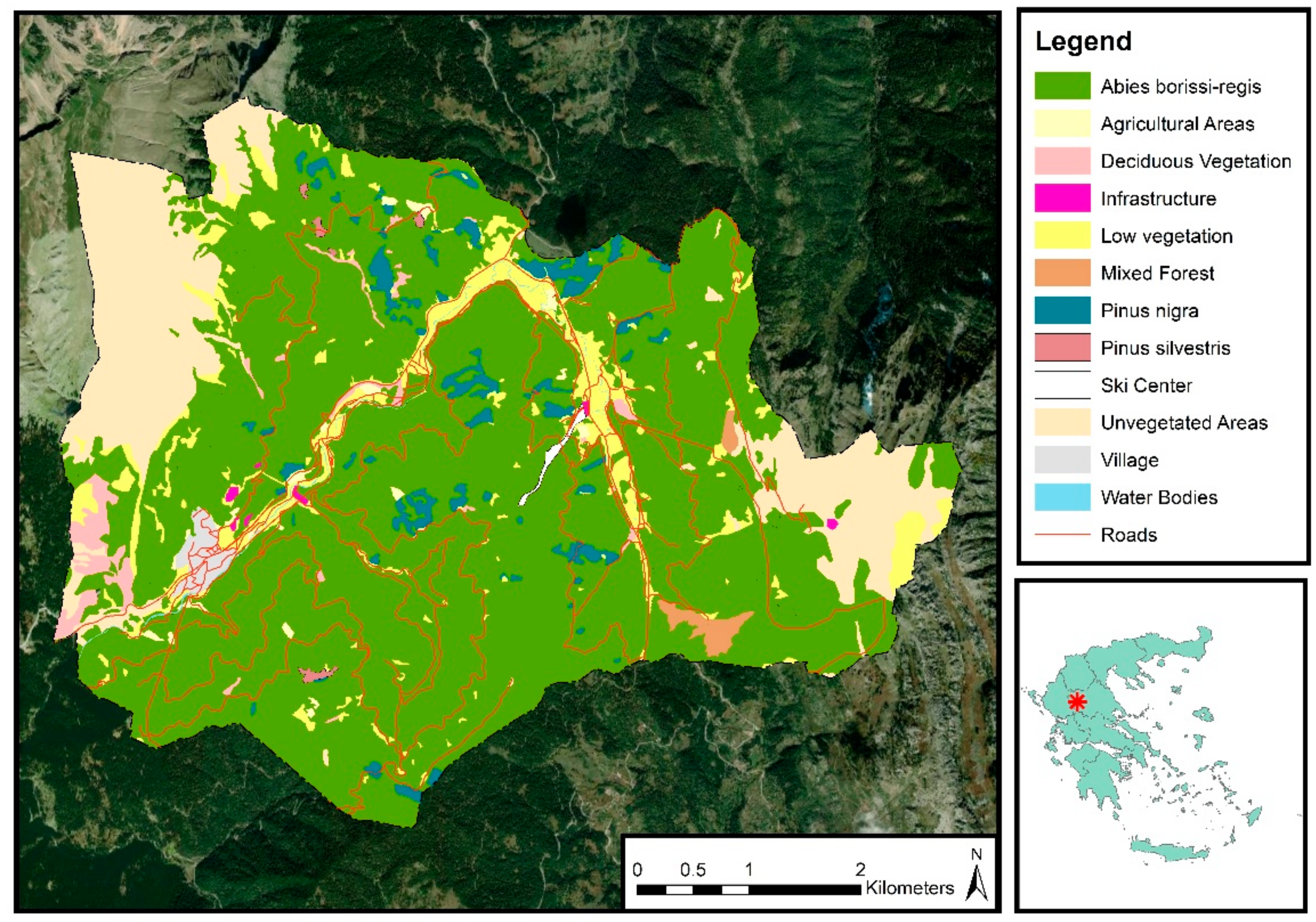
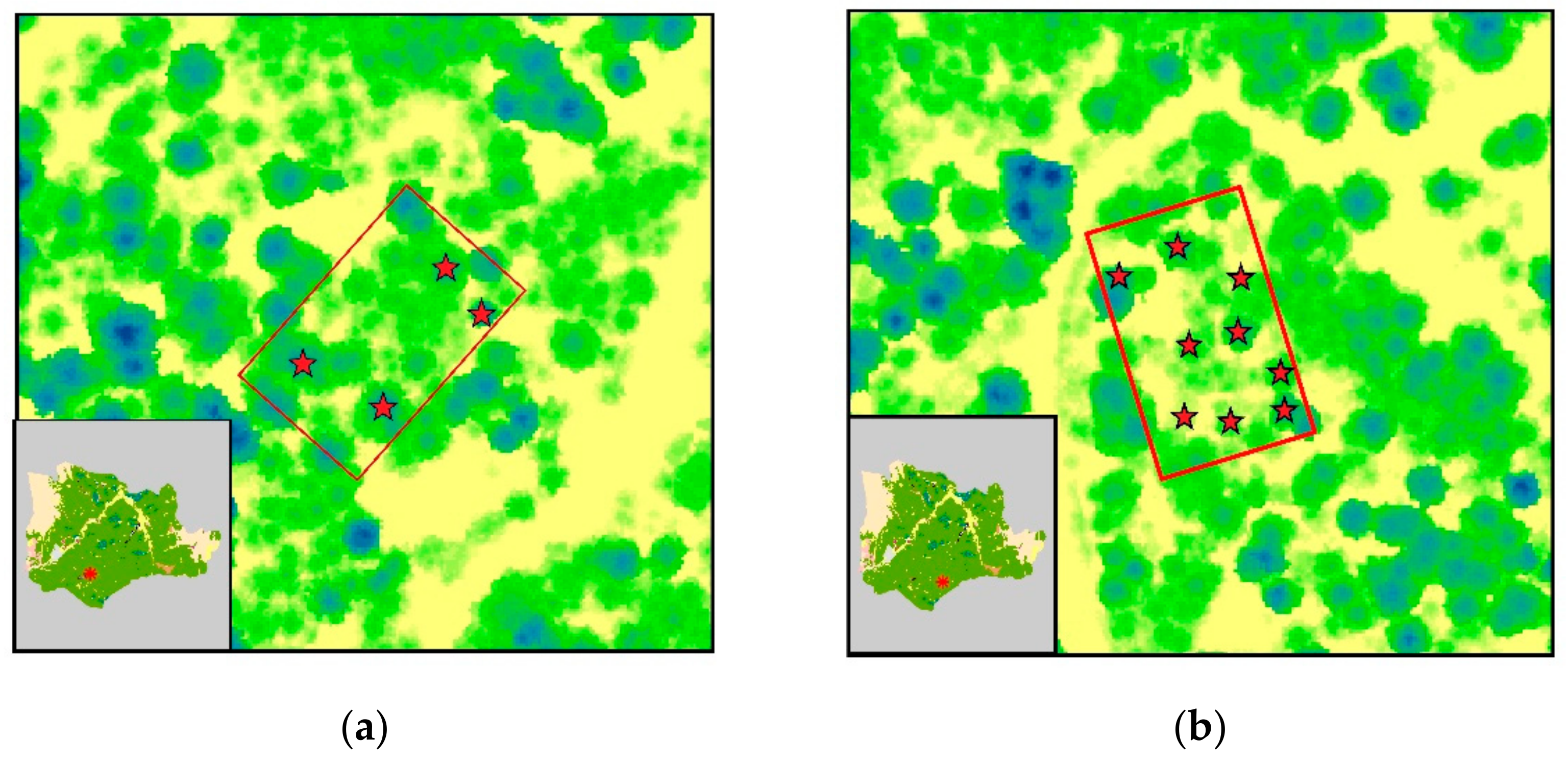
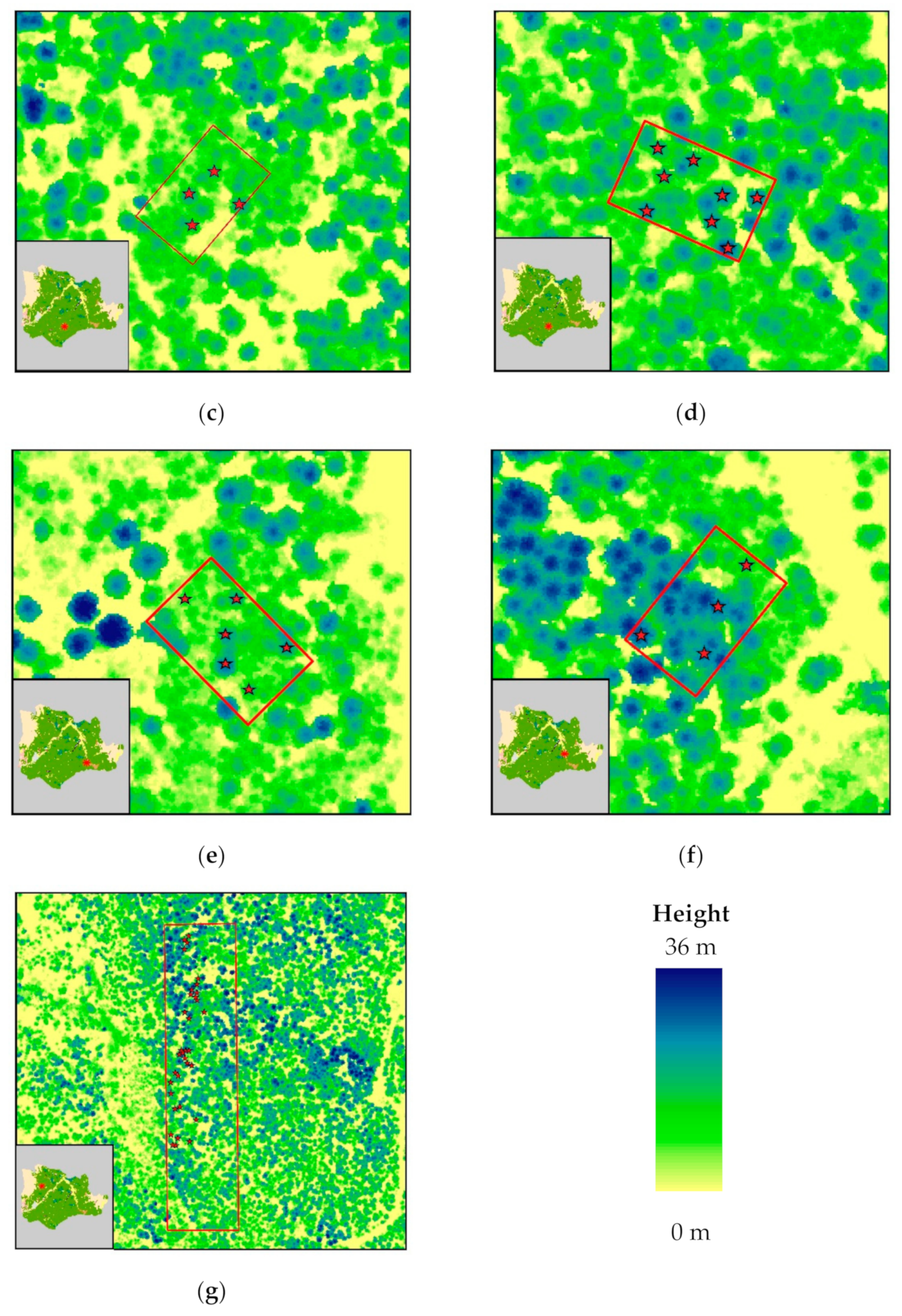


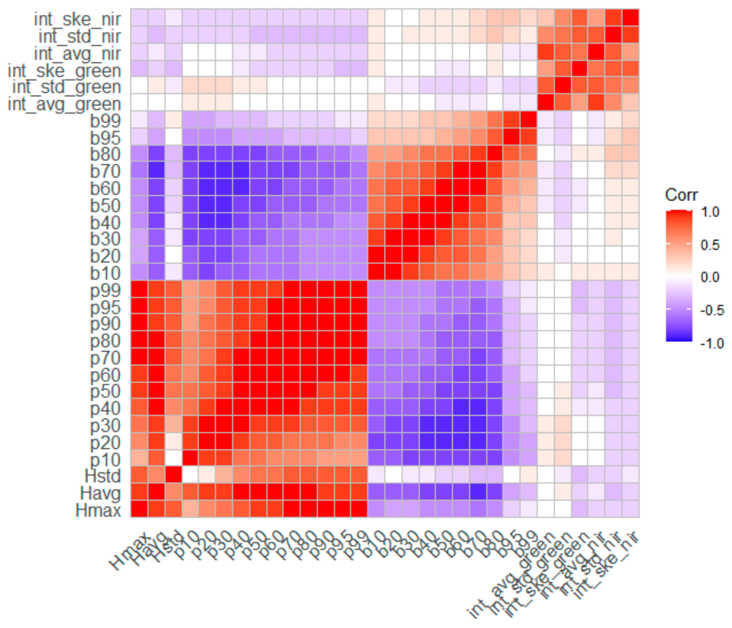
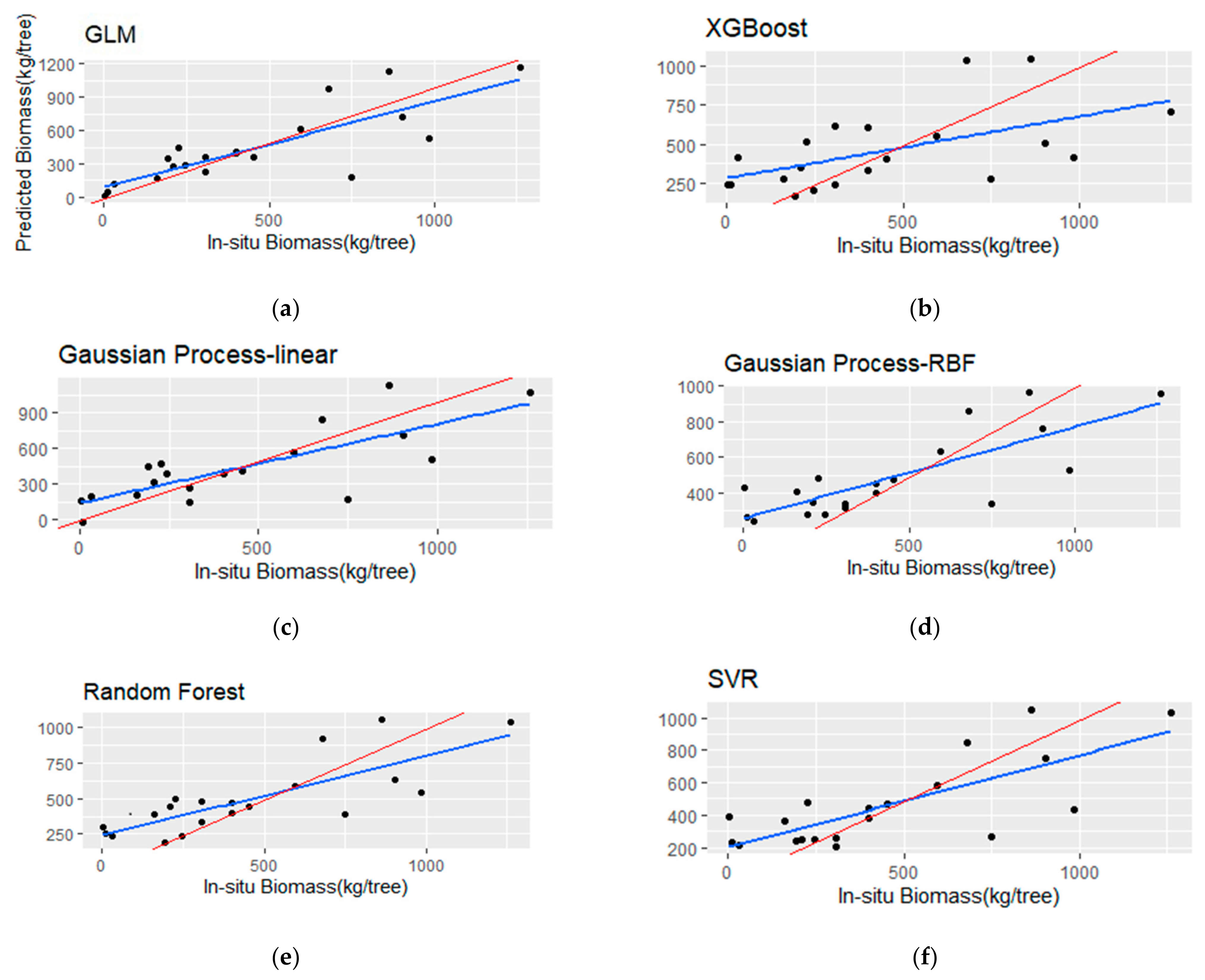
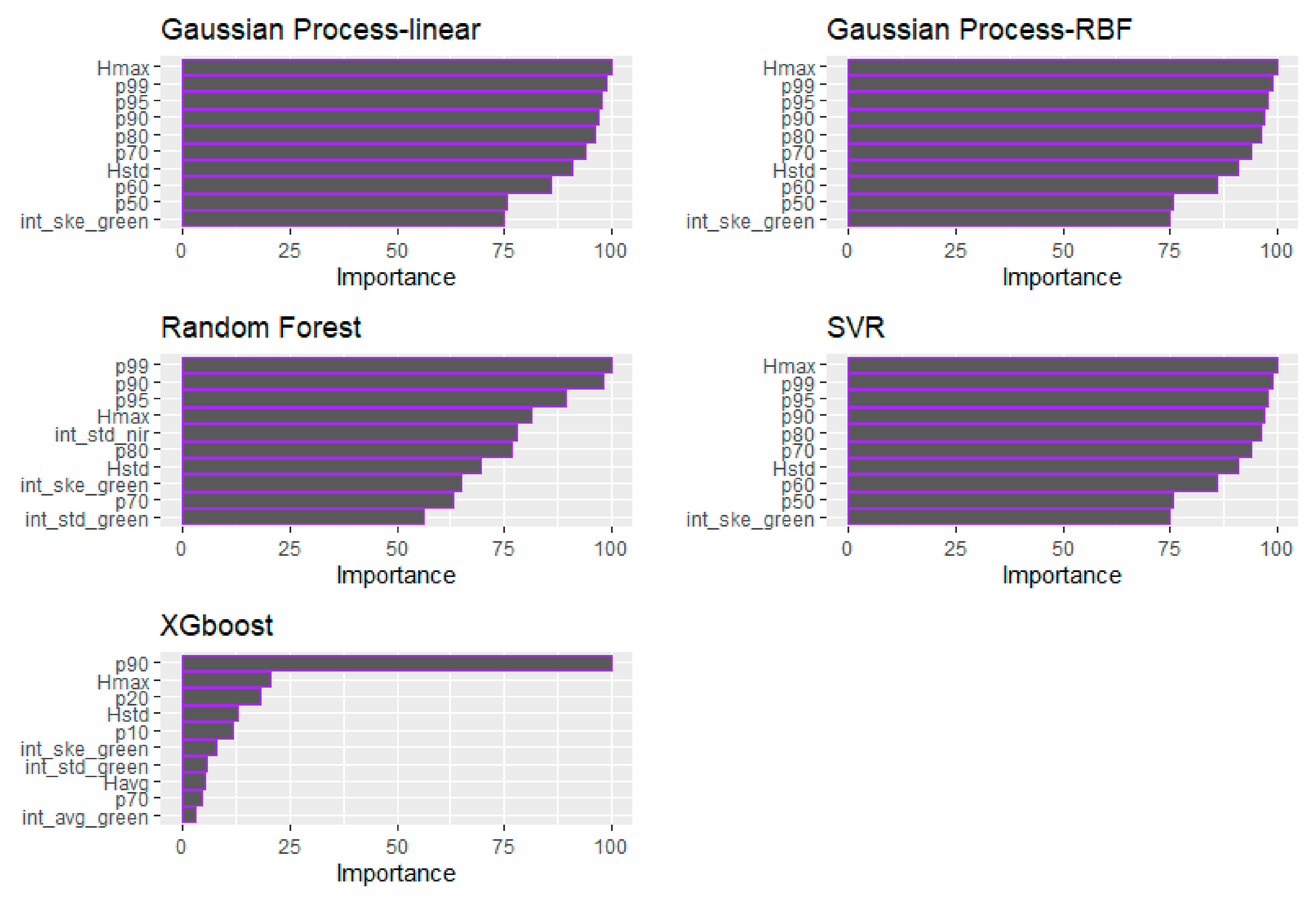
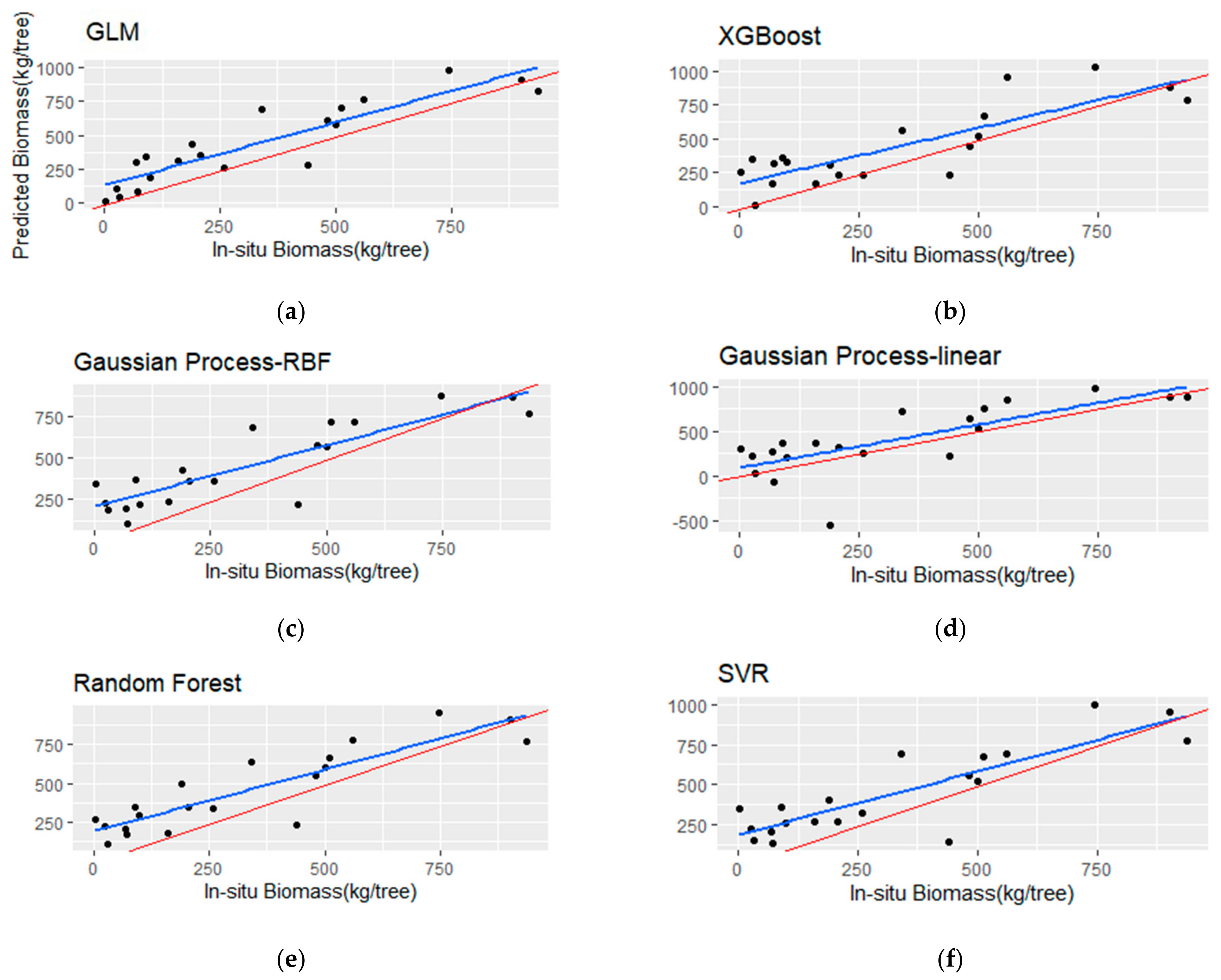

Publisher’s Note: MDPI stays neutral with regard to jurisdictional claims in published maps and institutional affiliations. |
© 2021 by the authors. Licensee MDPI, Basel, Switzerland. This article is an open access article distributed under the terms and conditions of the Creative Commons Attribution (CC BY) license (https://creativecommons.org/licenses/by/4.0/).