The Development and Application of Machine Learning in Atmospheric Environment Studies

Abstract

Machine learning (ML) plays an important role in atmospheric environment prediction, having been widely applied in atmospheric science with significant progress in algorithms and hardware. In this paper, we present a brief overview of the development of ML models as well as their application to atmospheric environment studies. ML model performance is then compared based on the main air pollutants (i.e., PM_2.5, O₃, and NO₂) and model type. Moreover, we identify the key driving variables for ML models in predicting particulate matter (PM) pollutants by quantitative statistics. Additionally, a case study for wet nitrogen deposition estimation is carried out based on ML models. Finally, the prospects of ML for atmospheric prediction are discussed.

1. Introduction

The atmospheric environment is closely related to human health, as a high level of air pollutants can cause various diseases. For example, excessive inhalation of PM increases the risk of respiratory and heart disease [1], and lengthy exposure to O₃ has a detrimental effect on human lung function, leading to asthma as well as other serious cardiopulmonary diseases [2]. Therefore, the prediction of the atmospheric environment is essential for guiding both policy-making and personal daily outings. Atmospheric prediction methods can be classified into two main types: statistical models (including machine learning (ML) models and typical statistical models such as Land-Use Regression [3] and Geographically Weighted Regression (GWR) [4,5]), and numerical models (e.g., chemical transport models [6], box models, Lagrangian/Eulerian Models, Computational Fluid Dynamics (CFD) models and Gaussian models [7]). As an important part of statistical models, typical statistical models are designed for specific regression tasks related to geographic space using geo-statistical modeling, such as local geographic weighted calculation in GWR [4], and land-use features derived from the Geographic Information System (GIS) [3,5,8]. This kind of model is cost-effective and useful, but the major disadvantage is the limited nonlinear-fitting capability [9]. Another part with great application potential is machine learning (ML) models, which includes tree models, artificial neural networks, etc. Numerical models were popular and convincing in the past according to scientific or empirical deterministic equations based on atmospheric physical and chemical mechanisms. However, due to the limited understanding of complex physical and chemical mechanisms, the development of numerical models has been slow. In addition, the computational costs of numerical models are high, and pollution prediction results are often not available in a timely fashion. In recent years, with the rapid development of computational hardware and algorithms, machine learning (ML) has aroused widespread interest and started to be applied in academia and industry due to its powerful model-fitting capability, universality, denoising capability, and portability [10,11,12]. ML models combine the advantages of high computational efficiency and better nonlinear-fitting capability, making it a suitable complementary tool when the performance of numerical models is not satisfactory. In view of the current limited understanding of atmospheric physical and chemical mechanisms, ML models provide an effective alternatively way to simulate the atmospheric environment, especially for time-limited applications. Owing to the increasingly important prospect of ML applications in the atmospheric environment, we conducted this review.

As a branch of ML, deep learning has received special research attention. Before the 2010s, the main form of deep learning was artificial neural networks (ANNs) with shallow layers [13]. After AlexNet [14] won the ImageNet competition in 2012, researchers started to realize the importance of “deeper” neural networks, opening a new era of deep learning innovation. The detailed development of this area is introduced in Section 3.

Many aspects are involved in studies of the atmospheric environment: the sources and sinks of atmospheric pollutants [15,16], meteorological influences [17,18], physical transport [19,20], chemical formation and transformation [21,22], and so on. In the above research fields, numerical models are generally a suitable study approach, while statistical and ML models are applied mostly to air-pollutant prediction (e.g., PM_2.5, O₃, and NO₂). Specifically, ML models are widely applied in remote sensing studies, which can be summarized into three main types:

• Remote sensing data processes. The processes include data fusion and downscaling [23,24,25,26], missing-information filling and reconstruction [27,28], image dehazing [29] and despeckling [30], and data registration [23,24,31,32];
• Classical application using remote sensing data. The application includes image classification and segmentation (e.g., land-use and land-cover classification [33,34]), object detection (clouds [35], buildings [36], vehicles [37], landslides [38], trees [39], and so on), and change detection [40];
• Further application in the earth system. As a kind of universal approximation estimation algorithm, ML models have gained wide application in earth-system studies by using remote sensing data, such as atmospheric-pollutant prediction (including gas [41,42,43] and particulate matter pollutants [44,45,46,47]) or atmospheric-parameter retrieval and correction (e.g., Aerosol Optical Depth (AOD) retrieval and error correction [48], planetary boundary layer height estimation [49,50], aerosol chemical composition classification [51,52]), agricultural and forest prediction (e.g., yield prediction for different crops [53,54], forest habitats [55]), other parameter estimation or prediction in the earth system (e.g., land surface temperature (LST) [56,57], precipitation [58], soil moisture [59], evapotranspiration [60], biomass [61,62]), and so on.

In this review, we focus on ML model applications to air-pollution prediction. Therefore, we selected the prediction of atmospheric pollutants, especially studies using remote sensing data and atmospheric parameters directly related to atmospheric pollution, such as aerosol chemical composition classification. In addition, as an important sink of air pollutants, deposition is closely associated with air pollutants and meteorological conditions, as in the process of washout of particulate chemicals [63] and the dry deposition of aerosols by turbulent diffusion [64]. Considering that few studies have applied ML models to deposition, and many studies have been conducted on applications to atmospheric pollutants, a case study applying ML models to simulate nitrate wet deposition was carried out as an innovative point in this review.

The main objective of this paper is to:

• Introduce the development of ML models, especially for prediction;
• Review the application of ML models to atmospheric pollutants, including model classification, ML model performance, and identification of key variables;
• Conduct a case study that applies ML to deposition, in the hope of gaining further insight into the suitability of ML models for deposition estimation;
• Discuss the prospects of ML models for the study of atmospheric pollution.

2. Literature Search

We used Web of Science and Google Scholar for a literature search and set 2000–2020 as the search period. There were three steps in the collection of literature. The first search keywords included three parts: machine learning (deep learning, artificial intelligence), atmospheric pollution (air quality, air pollutant, air pollution), and prediction (estimation, forecast). Furthermore, a supplementary search was conducted using new keywords based on the previous search results. The new keywords included two parts: models (e.g., tree model, neural network) and pollutants (e.g., PM_2.5, O₃). Particularly, since the aerosol feature (detection, classification) is an important research field directly related to atmospheric pollution state, we used keywords including two parts: machine learning (deep learning, artificial intelligence) and aerosol classification (identification). Finally, 276 publications were collected after the three-step search process for the following statistics and analysis.

3. Overview of Machine Learning Development

ML models can be classified into several types depending on the task objectives, such as regression, classification, reinforcement learning [65], generative models [66], and so on. Since this review gave priority to atmospheric pollution prediction, we introduced the general development timeline of ML models mainly for models that can be used in regression prediction, particularly current popular models.

Regarding ML models available for regression prediction, all ML models in the collected research were classified into 4 categories: traditional convex optimization-based models (TCOB models), tree models, linear regression (LR), and modern deep-learning structure models (modern DL structure). The development timeline with selected milestones according to our classification is shown in Figure 1.

• Traditional convex optimization-based model

Two main model types are included in the TCOB model group: Support Vector Machine (SVM) and artificial neural networks (ANNs). The optimization algorithms of SVM and ANNs are based mostly on convex optimization (e.g., a stochastic gradient descent algorithm). Essentially, these two models add nonlinear data transformation based on a linear model. In addition, the methods of data transformation are different in SVM and ANNs: SVM transforms the data by means of kernel functions, while ANNs use activation functions.

The development of SVM can be divided into two stages, non-kernel SVM and kernel SVM [67,68], the latter of which is commonly applied today. The kernel function transforms input features from a low dimension to a higher dimension, simplifying the mathematical calculations in the higher-dimensional space. In practice, linear, polynomial, and Radial Basis Function (RBF) kernels are three commonly used model kernels. Kernel selection depends on the specific tasks and model performance.

Multiple Layer Perceptron (MLP), also called Back Propagation Neural Network (BPNN) [69], is the simplest neural network in this model group. MLP contains three types of layers inside: the input layer, the hidden layer, and the output layer. The input layer is a one-dimensional layer that passes independent variables organized into the network. The hidden layer receives data from the input layer and processes by a feedforward algorithm. All parameters (including the weight and bias between two adjacent layers) in the network are optimized by a backpropagation algorithm. In the training stage, the prediction result is passed to the output layer after each epoch, and network parameters are updated to better fit the predictions. In the validation or testing stage, the network parameters are frozen and make predictions directly.

After MLP was proposed, a lot of artificial neural networks (ANNs) were developed from the 1970s to the 2010s, such as the Radial Basis Function Network (RBFN) [70], ELMAN network [71], General Regression Neural Network (GRNN) [72], Nonlinear Autoregressive with Exogenous Inputs Model (NARX) [73], Extreme Learning Machine (ELM) [74], and Deep Belief Networks (DBN) [75]. One distinctive characteristic of these models is that they are relatively shallow due to the limited computing power when the models were proposed and their artificial design. For example, RBFN contains a Gaussian activation function inside the network, which is not a suitable design for a “deep” network. Furthermore, among ANNs, more layers in the network do not always mean improved prediction performance; sometimes, performance even deteriorates. Even so, ANNs are currently still effective tools for atmospheric pollution prediction due to the simplicity of model application and powerful model performance.

2.

Tree models

The development of tree models went through two stages: basic models and ensemble models. Basic models include ID3 [76], C4.5 [77], and CART [78]. The differences between them lie in the method of selecting features and the number of branches in the tree. We will not introduce the algorithms mathematically here, as they can readily be found. As a further development of basic tree models, ensemble tree models are key to the maturity of this group of ML models. There were two ensemble ideas in the history of development: bagging and boosting. The representative bagging model is the random forest (RF) [79], which develops n sub-models from the original input data and makes a prediction by voting. The two main ideas in boosting are changing the sample weight, and fitting the residual error according to the loss function during the training stage. AdaBoost [80] uses the former idea, whereas the Gradient Boosting Decision Tree (GBDT) [81], also called the Gradient Boosting Model (GBM), uses the other idea. For now, GBDT has been improved and developed into different models, such as XGBoost [82], LightGBM [83], and CatBoost [84], which have been widely used for classification as well as regression tasks.

3.

Linear regression

This group includes multiple regression (MLR), the Autoregressive Integrated Moving Average model (ARIMA), ridge regression [85], Least Absolute Shrinkage and Selection Operator (LASSO) [86], Elastic Net [87], and Generalized Additive Model (GAM) [88]. These models were originally designed to solve regression tasks. From the perspective of ML, ridge regression, LASSO, and Elastic Net are for the regularization of linear regression. ARIMA is a time-series function transforming unstable time series into stable series for model fitting; GAM as described here refers specifically to GAM for regression, where the target variable is the sum of a series of subfunctions. The function can be expressed as follows:

$$y={\displaystyle \sum }_{i=1}^n{f}_i$$

(1)

$f_i$ can be any function here.

As can be seen in Figure 1, LR has a long history of development. However, the innovation of model algorithms has stagnated since Elastic Net was proposed. One important reason for this is the limited nonlinear-fitting ability of this group.

4.

Modern deep-learning structure models

Modern DL structure models are another important part of deep learning that evolved from the development of ANNs, which are redesigned based on MLP considering the characteristics of the prediction tasks and input data. Modern DL structure models include mainly a convolutional neural network (CNN) [89] and a recurrent neural network (RNN) [90]. CNN contains a feature-capturing filter module called a “kernel” to catch local spatial features, thus making substantial connections between neighboring layers that are sparser compared to the dense connections inside MLP. This design makes optimization and convergence of the network easier. CNN has developed many network structures with innovative model design concepts, such as AlexNet (network goes “deeper”) [14], VGG (doubles the number of layers, half the height and width) [91], ResNet (skip connection) [92], and GoogLeNet (inception block) [93]. These networks can not only be applied directly to prediction tasks, but also provide modern ideas for future network design.

Compared to CNN, RNN is better for capturing temporal relationships in a time series. This group of models retains historical data in the “memory” unit and passes them into the network in the following training. The classical RNN simply passes history information from the last time step into the network along with input data in the current time step. However, this original “memory” unit design leads to a terrible problem: a vanishing gradient, which hinders the successful training of the model. Advanced RNN-based structures such as the long short-term memory network (LSTM) [90] and gated recurrent units (GRU) [94] significantly alleviate this problem with structure modification. These advanced RNNs are now more widely applied compared to the original RNN.

During the development of modern DL structure models, several improved model components were proposed, which efficiently improved the performance of both ANNs and modern DL structure models. For instance, a sigmoid activation function was replaced by the Rectified Linear Unit (ReLU) [95] or LeakyReLU [96] in most regression tasks; the dropout method [97] was usually applied in the model training stage to alleviate overfitting; Adam [98] and weight decay regularization [99] are commonly used in network optimization.

4. Machine Learning Application to Atmospheric Pollution

The analysis of the application of ML models to atmospheric pollution includes three parts:

• Analysis of the ML application trend by the annual number of publications, and the pollutants of concern;
• Comparison of ML model prediction performance;
• Design of a scoring system to explore key variables in ML models.

4.1. ML Application Trend

The annual trend in the number of publications applying ML models to atmospheric pollution from 2000 to 2020 was analyzed according to the literature collection rules. Due to the stable trend during 2000–2015, the number of studies every five years is presented for this period. After 2015, since the proportion of model applications and total number of publications changed significantly from year to year, we depict the total number and model contributions for every year. In addition, an analysis of the proportion of air-pollutant species based on the research collection has also been conducted, and these are shown together in Figure 2.

As presented in Figure 2, the number of papers on ML application to atmospheric pollutants stabilized at around 10 or fewer until 2016, with TCOB models as the main ML model type in this period. After 2017, the research count started to increase steeply, while the share of different ML models changed significantly at the same time. The proportion of tree models increased rapidly in 2017–2020, from 15.8% to 23.4%. Compared with tree models, the growth of modern DL structure models appeared later after 2019, contributing 17.2% in 2020. In addition, the proportion of TCOB models decreased to less than 50% (26.6–44.4% in 2018–2020) after 2017, implying that the development of ML application to air pollution began to be more diverse. Another obvious increasing model type was ensemble models, from 5.3% to 28.1% during 2017–2020. It is worth noting that the ensemble models mentioned here do not include bagging or boosting tree models, but rather refer to the aggregation of multiple ML model types by voting, stacking, or bagging. As for LR, this model group accounted for a small proportion during the whole study period.

For atmospheric species, the three most studied species were PM_2.5, PM₁₀, and O₃, contributing 34.0%, 19.0%, and 17.8%, respectively. Other popular predicted pollutants included NO₂, AQI, SO₂, and CO. It is evident that the common predicted species in this review are important indicators for air quality monitoring networks regardless of country. On the one hand, these indicators represent the general pollution level in the atmospheric environment. On the other hand, indicators in the monitoring network suggest that data availability and quality control are guaranteed compared to other data, which is important for ML modeling. Detailed annual species proportion is depicted in Figure S1. The proportion of PM_2.5 increased after 2015, then stabilized during 2016–2020 (33.3–50.0%). The general proportion of PM₁₀ declined, especially in recent years (from 20.0% to 6.9% in 2018–2020). O₃ had a decreasing trend during 2010–2019 (from 50.0% to 7.8%), but the contribution was elevated in 2020 (18.4%), indicating rising concerns about ozone. Moreover, NO₂ and AQI have increased slightly since 2017. In general, due to the increased amount of research, the diversity of air-pollutant studies has increased compared to five or ten years ago.

4.2. Model Performance

From Section 3, it is found that different kinds of ML models, such as TCOB models, tree models, and modern DL structure models, are widely applied at present. For atmospheric pollution modeling, model performance with different pollutants needs to be explored, so as to provide a reference and guidance for future air-pollution prediction research. For this purpose, we completed a statistical analysis of model-evaluation metrics from the copious publications collected in this review.

Various metrics were used in different studies, such as root mean square error (RMSE), correlation coefficient (CORR), mean square error (MSE), mean absolute percentage error (MAPE), index of agreement (IOA), normalized root mean square error (NRMSE), and so on. According to the metric availability calculated, two indicators were available for model performance analysis: CORR (63.9%) and RMSE (73.8%). CORR was selected as a statistical indicator for the following reason. In our study, evaluation indicators were collected from different research based on different datasets from different regions. Indeed, absolute metrics are not comparable between unfixed datasets. For example, RMSE of 10 μg/m³ is probably not a significant error in a dataset averaging 1000 μg/m³, while it would be significant in another dataset averaging 20 μg/m³. Therefore, CORR rather than RMSE was selected as the indicator of model performance in our study. Furthermore, since most studies used absolute error as the modeling loss function, there was no need to worry about the situation in which CORR is high and the ratio between prediction and observation deviates from 1. Most studies adopted 1 day or 1 h prediction horizon (50.7% and 37.9%, respectively). The prediction time step in all collected metrics was 1 step.

All collected studies were divided according to model type, and average CORR values were calculated for three main atmospheric pollutants: PM_2.5, PM₁₀, and O₃, as shown in Figure 3. Clearly, modern DL structure models had the highest CORR values for all main pollutants, with 0.94, 0.87, and 0.89 for PM_2.5, PM₁₀, and O₃, respectively. The performance of the TCOB models and tree models was similar, with slight advantages and disadvantages with different species. From a species perspective, PM_2.5 was the most successfully modeled species, and two other models provided good prediction performance in addition to modern DL structure models (tree models 0.91, and TCOB models 0.87). Furthermore, three model types showed good performance in modeling O₃ in addition to modern DL structure models (tree models 0.86, and TCOB models 0.82). For PM₁₀, modern DL structure models performed the best, followed by TCOB models and tree models with the same metrics (0.80). Overall, modern DL structure models showed strong modeling capability for atmospheric pollution prediction, while TCOB models and tree models performed at a similar relatively high prediction level. Moreover, LR failed to provide good performance, especially for PM₁₀ and O₃ (0.67 and 0.69, respectively).

4.3. Key Variable Identification

As with numerical models, various input variables related to prediction are required for ML modeling. In the atmospheric environment, various factors (e.g., meteorological conditions, pollution emissions) affecting pollutant generation, transport, chemical transformation, and deposition during the atmospheric lifetime are strongly associated with atmospheric pollution [6,100,101,102]. These factors are significantly effective in atmospheric pollution modeling. Essentially, ML models make a prediction by exploring the connection between input variables and target pollutants. In numerical models, this process is accomplished by deterministic equations. Unlike the artificial equation design in numerical models, the goal of ML models is to simulate the interrelationship between factors in the atmospheric environment by adjusting model internal parameters based on the provided datasets. This process is called “learning”. Several kinds of factors are used as input variables for air-pollutant modeling:

• Meteorological variables, e.g., temperature, relative humidity, pressure, wind speed, precipitation, and so on.
• Pollutant variables. The most common variables are pollutant data from observation sites. Observation data are usually set as prediction targets. Due to the relationship between different pollutants, observations can also be used as input data for predictive models. Another kind of pollutant variable is satellite data, such as Aerosol Optical Depth (AOD), Top of Atmosphere (TOA) reflectance, and so on.
• Auxiliary variables, including temporal variables (e.g., month of the year, day of the month, and mathematical transformation), spatial variables (e.g., longitude, latitude, and mathematical transformation), elevation, land cover, and social and economic data (e.g., GDP, nightlight brightness, road density).
• Historical data, specifically referring to time-series data before the time point to be predicted, or spatial data near the location to be predicted. In this case, the observation values become both input variables and output targets. Whether they are used as input variables or output targets depends on the predicted time point and the station location. The number of previous time steps depends on your datasets, model types and the characteristics of your tasks. For example, several studies indicated that time series at shorter lags (e.g., one or two lags) are better for ML modeling [103,104,105,106]. However, for some ML structures with powerful capability of temporal information extraction (e.g., LSTM, GRU), suitable longer lags were better for the model performance [107,108].

Due to the “learning” nature of ML models, variables described above are not always necessary for pollution modeling. In addition, the “learning” of ML is not intuitive for humans, which makes it less convincing [109]. Therefore, it is important to identify key variables for model prediction, whether for better understanding of the model or for gaining better model performance.

In our study, the key variables for ML models identified in previous research were collected. However, the driving variables for ML models varied in different studies. Accordingly, a scoring system was designed for variable importance to quantitively present the importance of input variables. The detailed scoring function is shown below:

$$I{S}^i={\displaystyle \sum }_{j=1}^N{a}_j^i\times r_j^i$$

(2)

$I{S}^i$ presents the importance score of variable $i$; $a_j^i$ means the number of papers that rank variable $i$ as the $j$th important factor; $r_j^i$ presents the scoring point of variable $i$. In this study, the top-three most important variables were considered and assigned different scoring points: $r_1^i=3$, $r_2^i=2$, $r_3^i=1$, respectively. Finally, all scoring points were summed together for each collected variable.

Researchers tend to select variables during their study regardless of whether they are shown in their studies. Therefore, a new indicator was counted, $V{C}^i$, the number of times that factors were used in all research, to denote the popularity of a variable in pollutant prediction.

Considering the limited number of studies, PM_2.5 and PM₁₀ were combined as PM pollutants and statistical analysis was then conducted on the variable importance between different ML models based on two indicators: $I{S}^i$ and $V{C}^i$. According to the ML model classification, all research results were divided into four model groups: TCOB models, tree models, LR, and modern DL structure models. As presented in Figure 4, variable importance varied from model to model. Since PM_2.5 and PM₁₀ were combined, both the PM component (PM_2.5 or PM₁₀) and “historical data” existed simultaneously in the results of the same model. PM_2.5 meant that the prediction target was PM₁₀, and vice versa. For tree models, AOD from satellite data was the most important variable, followed by history data, day of the year (DOY), and temperature (T). TCOB models were slightly different from tree models, with history data, PM₁₀ (for PM_2.5 target), and wind speed (WS) as the top-three variables. For LR, the significant variables included WS, PM₁₀ (for PM_2.5), and history data. For modern DL structure models, the most significant variable was history data. Overall, AOD data, the PM component (including history data and another component inside), and WS were the most important variables. In addition, we need to pay attention to some variables with low $V{C}^i$ but relatively high $I{S}^i$, such as DOY, NO₂, and NO in tree models, and traffic data in TCOB models. These variables are probably important to PM-pollutant prediction but have received little attention in previous studies. A full list of variable names is included in Table S1.

In our study, we noticed that remote sensing data played an important role in pollutant modelling. Since many satellite products published in recent years (e.g., Himawari 8/9 [110], Sentinel 5p [111], HY2B, and MetOp-C [112]), many studies did not utilize remote sensing data in their studies. In our collection, 75.0% of the studies applying satellite data for modeling were conducted since 2018. Besides, among the studies that have conducted the analysis of variable importance, 64.0% identified remote sensing data as the most important variables. As more satellite data are publicly released, these kind of data have great potential to improve the model performance.

5. Case Study: ML Application to Nitrate Wet Deposition Estimation

From the systematic review of atmospheric pollutants in Section 4, ML has been increasingly applied in the prediction or estimation of air pollutants, obtaining good performance, especially for PM and ozone. It is well known that pollution processes in the atmospheric environment are very complex, including air-pollutant generation, transport, chemical transformation, decomposition, and deposition. However, most studies focus on common atmospheric pollutants, such as PM, O₃, NO₂, SO₂, and CO. As an important sink of atmospheric pollutants, deposition pollution has seldom been predicted or estimated by applying ML models, and the common simulation method for deposition has been numerical models such as the global 3-D model from the Goddard Earth Observing System (GEOS), GEOS-Chem [113], and the chemical transport model developed at Meteorological Synthesizing Centre-West (MSC-W) from the European Monitoring and Evaluation Programme (EMEP), the EMEP MSC-W chemical transport model [114].

Therefore, in this section, several ML models were applied to estimate nitrate wet deposition in Guangdong province in China, aiming at seeking the applicability of ML models to deposition simulation. We selected one model in each model group classified in Section 3 as a representative model. Furthermore, we ran a numerical simulation case for comparison, which coupled the EMEP MSC-W chemical transport model with the Weather Research and Forecasting Model (WRF, v3.9.1) (WRF-EMEP) in the same period in Guangdong province. Additionally, due to the discontinuity of the time series in the deposition dataset, RNN was not considered in this case study. Finally, CNN, MLP, RF, MLR, and WRF-EMEP were selected for deposition modeling.

5.1. Study Area and Data

5.1.1. Study Area

Guangdong province lies in the south of China, with an area of 1.79 × 10⁵ km². There are 21 cities in this area, including Guangzhou, Shenzhen, Zhuhai, Shantou, and others. Annual precipitation varies from 1000 to 2000 mm under the influence of a subtropical monsoon climate. In our study, hourly ${\mathrm{NO}}_3^{-}$ wet precipitation measurements were collected from 25 sites from 2010 to 2017 in this region, with reliable quality control complying with the Collection and Preservation of the wet precipitation sample (GB/T 13580.2-1992) and the determination of fluoride, chloride, nitrite nitrate, sulphate in the wet precipitation—ion chromatography (GB/T 13580.5-1992). For modeling, monthly fluxes were calculated based on the following equations:

$$C_w={\sum }_{i=1}^n\left(C_i{M}_i\right)/{\sum }_{i=1}^n{M}_i,$$

(3)

$$D_w=M_t{C}_w/100,$$

(4)

where $C_w$ is the volume-weighted mean concentration of wet N concentration (mg N L⁻¹) in a customized study period (a month, a year, or other period); $M_i$ is the amount of precipitation, and; $C_i$ is the concentration. $D_w$ is wet N deposition flux (kg N ha⁻¹) calculated by the factors of $M_t$, the total amount of precipitation (mm) over a period.

Finally, eight years (2010–2017) of monthly fluxes from 25 sites were obtained in Guangdong province as prediction targets in the present work. The site location can be seen in Figure S2.

5.1.2. Data

Meteorological data were obtained from the China Meteorological Forcing Dataset (CMFD) [115] (http://data.tpdc.ac.cn/en/data/1980e33d-8615-448c-80e3-cfcb635fb110/, accessed on 27 July 2021). CMFD is a high spatial–temporal resolution gridded near-surface meteorological dataset developed in China (0.1° × 0.1°). We selected seven variables at a monthly temporal resolution from CMFD as the input feature, including 2 m air temperature (temp), surface pressure (sp), specific humidity (shum), 10 m wind speed (wind), downward shortwave radiation (srad), downward longwave radiation (lrad), and precipitation rate (prep).

For satellite data, tropospheric NO₂ column vertical density (VCD) from the Peking University Ozone Monitoring Instrument NO₂ product (POMINO) [116], a satellite product retrieved from OMI (http://www.pku-atmos-acm.org/~acm/acmProduct.php/#POMINO, accessed on 20 July 2021), was selected. Specifically, the latest POMINO version, POMINO v2, was used as the input dataset, with higher accuracy than the previous version. Since the dataset was retrieved with 0.25° × 0.25° longitude–latitude coordinates, we resampled VCD at 0.1° × 0.1° resolution as the input feature.

The NO_x emission inventory from the Multi-resolution Emission Inventory for China (MEIC) [117,118], with a spatial resolution of 0.25° × 0.25°, was downloaded from Tsinghua University (http://meicmodel.org/, accessed on 26 July 2021). Like VCD, the NO_x emission inventory was resampled at 0.1° × 0.1° resolution.

For auxiliary variables, the month of the year (MOY) was selected as a temporal variable, and longitude and latitude as spatial variables. Considering the temporal continuity of the temporal variable, the month variables were transformed into sine form by Equation (5). Specifically, for month j:

$$MO{Y}^j=\sin \left(\frac{2\pi j}{12}\right),$$

(5)

We also considered the influence of topography. Elevation data (elev) were obtained from the Shuttle Radar Topographic Mission (SRTM, version 4) produced by NASA (https://srtm.csi.cgiar.org/, accessed on 9 August 2021).

5.2. Model Design

Convolutional neural networks (CNN) are one of the most popular deep-learning structures in the deep-learning family and have been widely used in computer vision areas, including image classification, target detection, semantic segmentation, and so on [119]. The greatest advantage of CNN is the spatial feature extraction capability due to the constraint of weight sharing in the well-designed convolutional filter. In this study, a CNN was developed to estimate nitrate wet deposition. The structure of CNN is presented in Figure 5. The CNN model was developed on Pytorch 1.9.1, and the version of Python was 3.7.11. The data preprocess and analysis were mainly based on Numpy and Pandas libraries.

Meteorological variables (temp, shum, wind, sp, prep, srad, lrad), emission data (NO_x emission), auxiliary parameters (lon, lat, elev, MOY), satellite data (VCD), and zero padding were grouped and reshaped into a 7 × 2 size for each grid point in Guangdong province. Then, observation data at each site and the grouped grid data were paired according to the smallest Euclidean distance as samples to construct the whole dataset. The prediction target (label) was the observation data, the monthly nitrate wet flux (one dimension); 30% of the dataset was used for validation by random sampling, and the remaining 70% was used for training. For the hidden layer, we designed three convolutional layers with 1 × 1 convolutional kernels, with variables in each sample consisting of the different types described in Section 4.3. The convolutional filters were initialized by Kaiming Initialization [120]. The number of filters doubled with the deepening of the layers (8, 16, and 32). After three convolutional layers, there were two fully connected layers with 64 neurons for each layer, in the hope of better fitting the prediction. Since the prediction in our study was a regression task, mean square error loss was selected as the loss function. In addition, a batch-normalization layer was added before each convolutional layer to reduce Internal Covariate Shift [121]. The Rectified Linear Unit (ReLU) was selected as the activation function in our network. Additionally, the Adam algorithm [98] was selected as the optimization method during the training step.

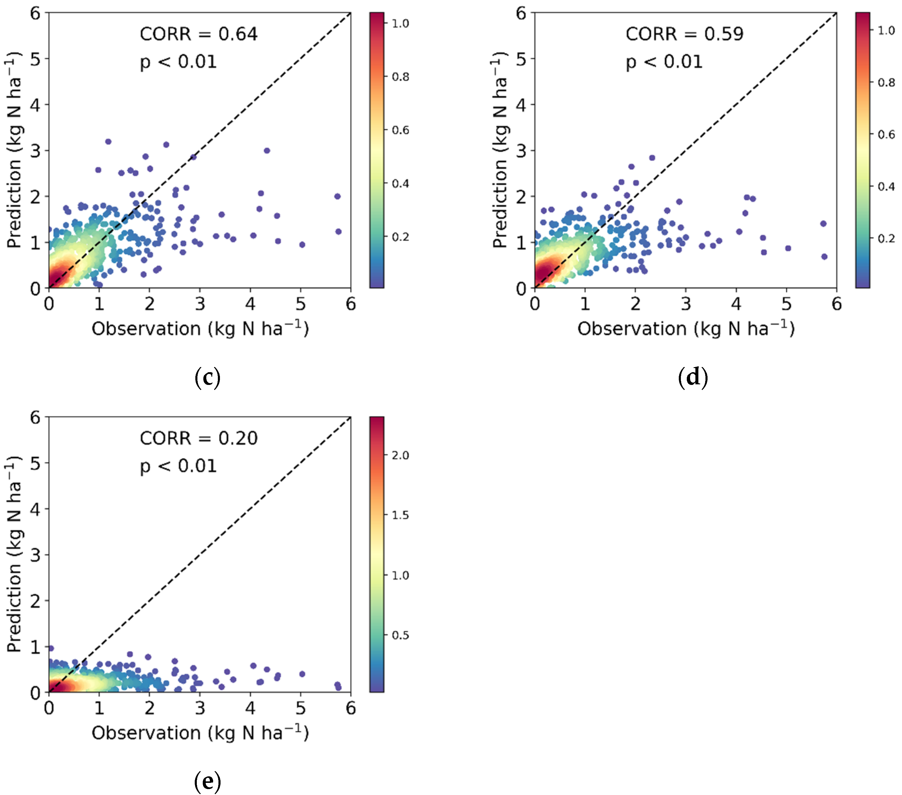
5.3. Performance Comparison

According to model selection at the beginning of this section, four ML models and one numerical model (WRF-EMEP) were trained with the same dataset introduced in Section 5.1. The performance of all models is shown in Figure 6 and

Table 1. Quantitative metrics of predictive models.

Model	CORR	RMSE	MSE	MAE
CNN	0.68	0.61	0.38	0.37
RF	0.65	0.64	0.41	0.38
MLP	0.64	0.64	0.41	0.39
MLR	0.59	0.68	0.46	0.41
WRF-EMEP	0.20	0.93	0.87	0.55

. Generally, all ML models showed significant correlation between observations and estimation fluxes (p-value < 0.01). CNN performed best (CORR = 0.68, RMSE = 0.61) compared to the other ML models (CORR = 0.59–0.65, RMSE = 0.64–0.68). For the fitting degree of the validation dataset, RF tended to overestimate or underestimate to a relatively large extent at some points. For MLR, more points with high values tended to be underestimated, as can be seen in Figure 6d. The numerical model (WRF-EMEP) performed worst (CORR = 0.20, RMSE = 0.93) in this case, significantly underestimating the deposition flux in most samples of the validation dataset, especially for some samples with high observation deposition flux. Therefore, for the case in this study, ML models provided more reasonable simulation results than the selected numerical model.

From Figure 6 and Table 1, it seems that the advantage of CNN was not significant compared to the other ML models. However, the robustness of each model was totally different, which can be reflected in the spatial simulation. Figure S3 shows a spatial estimation by the 4 ML models (Figure S3b–e), observations (Figure S3a), and WRF-EMEP model (Figure S3f) in July 2014. The estimation made by tree models (RF) showed some anomalous patches with high values and failed to show reasonable spatial distribution. Obviously, the RF model overfitted the local site in the central Pearl River Delta (PRD) despite the validation during model training. In addition, MLP and MLR presented high values in the margins of Guangdong province, which were not reasonable compared to the spatial distribution of observations. As for the result of numerical model WRF-EMEP, the high values in the central PRD were significantly underestimated. The estimation by CNN well reconstructed the spatial distribution of nitrate wet flux in Guangdong province, with the deposition center in the western and northern PRD. From the above analysis, most ML models failed to estimate nitrate wet flux well when the site estimation was generalized to area mapping estimation, except CNN, which could capture the spatial pattern of simulated nitrate wet deposition.

5.4. Spatiotemporal Distribution

Based on the model performance results, we selected CNN as the final ML model for nitrate wet deposition estimation. The annual mean spatial distributions of observations and model estimation are presented in Figure 7a,b, respectively. The estimation mapping result is well consistent with the spatial distribution of observation values, with the deposition center in the western and northern PRD. This general spatial pattern is similar to that in previous studies using numerical models [122]. Furthermore, spatial error analysis (RMSE) is conducted in Figure 7c. The main RMSE was concentrated at several sites with high deposition values (located mainly in the PRD), whereas errors at other sites were small. Moreover, annual total wet flux between the model estimation and observations is compared in Figure 7d. Overall, the model-estimated flux was slightly higher than observations, with smaller differences when the annual observation flux was high (2010, 2015, and 2016).

6. Future Prospects

The idea in current research applying ML models to atmospheric prediction is to stay at the application level. Most research has simply used ML models as a “black box” predictor or added sophisticated designs as a data processor, e.g., variable selection or transformation [123,124,125,126,127], predicted target decomposition [128,129,130,131,132], and spatiotemporal information addition [107,133,134,135,136]. Another application method is the ensemble approach [137,138]. Few studies have improved the internal structure of predictive models according to specific atmospheric pollution problems. In the artificial intelligence field, many classical DL structure models have been proposed based on specific problems, such as target detection (faster R-CNN algorithm) [139] and semantic segmentation (FCN algorithm) [140]. When considering atmospheric pollution prediction, ML models also need “customization” for model structure design, rather than simply designing the pre-process for input data and predictive targets, or hyperparameter optimization modification inside ML models.

One “customization” idea is coupling with numerical models. Today, numerical models have been well developed [141] and have become mainstream in atmospheric pollutant prediction, especially for regional- or national-scale prediction. Physics and chemical constraints inside the numerical models reflect atmospheric laws. Coupling these constraints to ML models (e.g., in a regularization-like way) is an important idea for improvement in the future. In fact, similar efforts have begun recently, such as solving partial differential equations [142] and emulating pollutants [143,144].

The addition of physical and chemical characteristics of atmospheric pollution to constrain the model will also improve model interpretability (the extent to which a cause and effect can be observed within a model) or explainability (the extent to which results can be explained in human terms). Due to the characteristic of “learning” in ML models, their interpretability is far from that of numerical models. However, quite a few studies have ignored interpretability or explainability, or they have explained model results based simply on variable importance [145,146,147]. For now, the effort toward model interpretability or explainability is not enough. This will become a crucial issue in the future when ML models are more widely studied and applied. Model designers should consider model interpretability when designing future ML models.

References

1. Turner, M.C.; Krewski, D.; Pope, C.A., III; Chen, Y.; Gapstur, S.M.; Thun, M.J. Long-term ambient fine particulate matter air pollution and lung cancer in a large cohort of never-smokers. Am. J. Respir. Crit. Care Med. 2011, 184, 1374–1381. [Google Scholar] [CrossRef]
2. Kampa, M.; Castanas, E. Human health effects of air pollution. Environ. Pollut. 2008, 151, 362–367. [Google Scholar] [CrossRef]
3. Liu, W.; Li, X.; Chen, Z.; Zeng, G.; León, T.; Liang, J.; Huang, G.; Gao, Z.; Jiao, S.; He, X. Land use regression models coupled with meteorology to model spatial and temporal variability of NO2 and PM10 in Changsha, China. Atmos. Environ. 2015, 116, 272–280. [Google Scholar] [CrossRef]
4. Song, W.; Jia, H.; Huang, J.; Zhang, Y. A satellite-based geographically weighted regression model for regional PM2.5 estimation over the Pearl River Delta region in China. Remote Sens. Environ. 2014, 154, 1–7. [Google Scholar] [CrossRef]
5. Wheeler, D.C.; Páez, A. Geographically weighted regression. In Handbook of Applied Spatial Analysis; Springer: Berlin/Heidelberg, Germany, 2010; pp. 461–486. [Google Scholar]
6. Lu, X.; Zhang, L.; Chen, Y.; Zhou, M.; Zheng, B.; Li, K.; Liu, Y.; Lin, J.; Fu, T.-M.; Zhang, Q. Exploring 2016–2017 surface ozone pollution over China: Source contributions and meteorological influences. Atmos. Chem. Phys. 2019, 19, 8339–8361. [Google Scholar] [CrossRef] [Green Version]
7. Holmes, N.S.; Morawska, L. A review of dispersion modelling and its application to the dispersion of particles: An overview of different dispersion models available. Atmos. Environ. 2006, 40, 5902–5928. [Google Scholar] [CrossRef] [Green Version]
8. Hoek, G.; Beelen, R.; De Hoogh, K.; Vienneau, D.; Gulliver, J.; Fischer, P.; Briggs, D. A review of land-use regression models to assess spatial variation of outdoor air pollution. Atmos. Environ. 2008, 42, 7561–7578. [Google Scholar] [CrossRef]
9. Liu, Y.; Goudreau, S.; Oiamo, T.; Rainham, D.; Hatzopoulou, M.; Chen, H.; Davies, H.; Tremblay, M.; Johnson, J.; Bockstael, A. Comparison of land use regression and random forests models on estimating noise levels in five Canadian cities. Environ. Pollut. 2020, 256, 113367. [Google Scholar] [CrossRef]
10. Zuo, R.; Xiong, Y.; Wang, J.; Carranza, E.J.M. Deep learning and its application in geochemical mapping. Earth-Sci. Rev. 2019, 192, 1–14. [Google Scholar] [CrossRef]
11. Deng, L.; Yu, D. Deep learning: Methods and applications. Found. Trends Signal Process. 2014, 7, 197–387. [Google Scholar] [CrossRef] [Green Version]
12. Yuan, Q.; Shen, H.; Li, T.; Li, Z.; Li, S.; Jiang, Y.; Xu, H.; Tan, W.; Yang, Q.; Wang, J. Deep learning in environmental remote sensing: Achievements and challenges. Remote Sens. Environ. 2020, 241, 111716. [Google Scholar] [CrossRef]
13. Yegnanarayana, B. Artificial Neural Networks; PHI Learning Pvt. Ltd.: New Delhi, India, 2009. [Google Scholar]
14. Krizhevsky, A.; Sutskever, I.; Hinton, G.E. Imagenet classification with deep convolutional neural networks. Adv. Neural Inf. Process. Syst. 2012, 25, 1097–1105. [Google Scholar] [CrossRef]
15. Pfaffhuber, K.A.; Berg, T.; Hirdman, D.; Stohl, A. Atmospheric mercury observations from Antarctica: Seasonal variation and source and sink region calculations. Atmos. Chem. Phys. 2012, 12, 3241–3251. [Google Scholar] [CrossRef] [Green Version]
16. Baker, D.; Bösch, H.; Doney, S.; O’Brien, D.; Schimel, D. Carbon source/sink information provided by column CO2 measurements from the Orbiting Carbon Observatory. Atmos. Chem. Phys. 2010, 10, 4145–4165. [Google Scholar] [CrossRef] [Green Version]
17. Bousiotis, D.; Brean, J.; Pope, F.D.; Dall’Osto, M.; Querol, X.; Alastuey, A.; Perez, N.; Petäjä, T.; Massling, A.; Nøjgaard, J.K. The effect of meteorological conditions and atmospheric composition in the occurrence and development of new particle formation (NPF) events in Europe. Atmos. Chem. Phys. 2021, 21, 3345–3370. [Google Scholar] [CrossRef]
18. Lee, J.; Kim, K.-Y. Analysis of source regions and meteorological factors for the variability of spring PM10 concentrations in Seoul, Korea. Atmos. Environ. 2018, 175, 199–209. [Google Scholar] [CrossRef]
19. Zhao, H.; Li, X.; Zhang, Q.; Jiang, X.; Lin, J.; Peters, G.P.; Li, M.; Geng, G.; Zheng, B.; Huo, H. Effects of atmospheric transport and trade on air pollution mortality in China. Atmos. Chem. Phys. 2017, 17, 10367–10381. [Google Scholar] [CrossRef] [Green Version]
20. Ma, Q.; Wu, Y.; Zhang, D.; Wang, X.; Xia, Y.; Liu, X.; Tian, P.; Han, Z.; Xia, X.; Wang, Y. Roles of regional transport and heterogeneous reactions in the PM2.5 increase during winter haze episodes in Beijing. Sci. Total Environ. 2017, 599, 246–253. [Google Scholar] [CrossRef]
21. An, Z.; Huang, R.-J.; Zhang, R.; Tie, X.; Li, G.; Cao, J.; Zhou, W.; Shi, Z.; Han, Y.; Gu, Z. Severe haze in northern China: A synergy of anthropogenic emissions and atmospheric processes. Proc. Natl. Acad. Sci. USA 2019, 116, 8657–8666. [Google Scholar] [CrossRef] [Green Version]
22. Wu, R.; Xie, S. Spatial distribution of ozone formation in China derived from emissions of speciated volatile organic compounds. Environ. Sci. Technol. 2017, 51, 2574–2583. [Google Scholar] [CrossRef]
23. Alparone, L.; Wald, L.; Chanussot, J.; Thomas, C.; Gamba, P.; Bruce, L.M. Comparison of pansharpening algorithms: Outcome of the 2006 GRS-S data-fusion contest. IEEE Trans. Geosci. Remote Sens. 2007, 45, 3012–3021. [Google Scholar] [CrossRef] [Green Version]
24. Ghamisi, P.; Rasti, B.; Yokoya, N.; Wang, Q.; Hofle, B.; Bruzzone, L.; Bovolo, F.; Chi, M.; Anders, K.; Gloaguen, R. Multisource and multitemporal data fusion in remote sensing. arXiv 2018, arXiv:1812.08287. [Google Scholar]
25. Shen, H.; Meng, X.; Zhang, L. An integrated framework for the spatio–temporal–spectral fusion of remote sensing images. IEEE Trans. Geosci. Remote Sens. 2016, 54, 7135–7148. [Google Scholar] [CrossRef]
26. Mou, L.; Zhu, X.; Vakalopoulou, M.; Karantzalos, K.; Paragios, N.; Le Saux, B.; Moser, G.; Tuia, D. Multitemporal very high resolution from space: Outcome of the 2016 IEEE GRSS data fusion contest. IEEE J. Sel. Top. Appl. Earth Obs. Remote Sens. 2017, 10, 3435–3447. [Google Scholar] [CrossRef] [Green Version]
27. Gavriil, K.; Muntingh, G.; Barrowclough, O.J. Void filling of digital elevation models with deep generative models. IEEE Geosci. Remote Sens. Lett. 2019, 16, 1645–1649. [Google Scholar] [CrossRef]
28. Zeng, C.; Shen, H.; Zhang, L. Recovering missing pixels for Landsat ETM+ SLC-off imagery using multi-temporal regression analysis and a regularization method. Remote Sens. Environ. 2013, 131, 182–194. [Google Scholar] [CrossRef]
29. Gu, Z.; Zhan, Z.; Yuan, Q.; Yan, L. Single remote sensing image dehazing using a prior-based dense attentive network. Remote Sens. 2019, 11, 3008. [Google Scholar] [CrossRef] [Green Version]
30. Shen, H.; Zhou, C.; Li, J.; Yuan, Q. SAR image despeckling employing a recursive deep CNN prior. IEEE Trans. Geosci. Remote Sens. 2020, 59, 273–286. [Google Scholar] [CrossRef]
31. Wang, S.; Quan, D.; Liang, X.; Ning, M.; Guo, Y.; Jiao, L. A deep learning framework for remote sensing image registration. ISPRS J. Photogramm. Remote Sens. 2018, 145, 148–164. [Google Scholar] [CrossRef]
32. Hughes, L.H.; Schmitt, M.; Mou, L.; Wang, Y.; Zhu, X.X. Identifying corresponding patches in SAR and optical images with a pseudo-siamese CNN. IEEE Geosci. Remote Sens. Lett. 2018, 15, 784–788. [Google Scholar] [CrossRef] [Green Version]
33. Rodriguez-Galiano, V.F.; Ghimire, B.; Rogan, J.; Chica-Olmo, M.; Rigol-Sanchez, J.P. An assessment of the effectiveness of a random forest classifier for land-cover classification. ISPRS J. Photogramm. Remote Sens. 2012, 67, 93–104. [Google Scholar] [CrossRef]
34. Talukdar, S.; Singha, P.; Mahato, S.; Pal, S.; Liou, Y.-A.; Rahman, A. Land-use land-cover classification by machine learning classifiers for satellite observations—A review. Remote Sens. 2020, 12, 1135. [Google Scholar] [CrossRef] [Green Version]
35. Liu, S.; Li, M.; Zhang, Z.; Xiao, B.; Cao, X. Multimodal ground-based cloud classification using joint fusion convolutional neural network. Remote Sens. 2018, 10, 822. [Google Scholar] [CrossRef] [Green Version]
36. He, N.; Fang, L.; Plaza, A. Hybrid first and second order attention Unet for building segmentation in remote sensing images. Sci. China Inf. Sci. 2020, 63, 1–12. [Google Scholar] [CrossRef] [Green Version]
37. Jin, X.; Davis, C.H. Vehicle detection from high-resolution satellite imagery using morphological shared-weight neural networks. Image Vis. Comput. 2007, 25, 1422–1431. [Google Scholar] [CrossRef]
38. Ji, S.; Yu, D.; Shen, C.; Li, W.; Xu, Q. Landslide detection from an open satellite imagery and digital elevation model dataset using attention boosted convolutional neural networks. Landslides 2020, 17, 1337–1352. [Google Scholar] [CrossRef]
39. Zheng, J.; Fu, H.; Li, W.; Wu, W.; Zhao, Y.; Dong, R.; Yu, L. Cross-regional oil palm tree counting and detection via a multi-level attention domain adaptation network. ISPRS J. Photogramm. Remote Sens. 2020, 167, 154–177. [Google Scholar] [CrossRef]
40. Khelifi, L.; Mignotte, M. Deep learning for change detection in remote sensing images: Comprehensive review and meta-analysis. IEEE Access 2020, 8, 126385–126400. [Google Scholar] [CrossRef]
41. Chan, K.L.; Khorsandi, E.; Liu, S.; Baier, F.; Valks, P. Estimation of surface NO2 concentrations over Germany from TROPOMI satellite observations using a machine learning method. Remote Sens. 2021, 13, 969. [Google Scholar] [CrossRef]
42. Liu, R.; Ma, Z.; Liu, Y.; Shao, Y.; Zhao, W.; Bi, J. Spatiotemporal distributions of surface ozone levels in China from 2005 to 2017: A machine learning approach. Environ. Int. 2020, 142, 105823. [Google Scholar] [CrossRef]
43. Requia, W.J.; Di, Q.; Silvern, R.; Kelly, J.T.; Koutrakis, P.; Mickley, L.J.; Sulprizio, M.P.; Amini, H.; Shi, L.; Schwartz, J. An ensemble learning approach for estimating high spatiotemporal resolution of ground-level ozone in the contiguous United States. Environ. Sci. Technol. 2020, 54, 11037–11047. [Google Scholar] [CrossRef]
44. Chen, Z.-Y.; Zhang, T.-H.; Zhang, R.; Zhu, Z.-M.; Yang, J.; Chen, P.-Y.; Ou, C.-Q.; Guo, Y. Extreme gradient boosting model to estimate PM2.5 concentrations with missing-filled satellite data in China. Atmos. Environ. 2019, 202, 180–189. [Google Scholar] [CrossRef]
45. Chen, G.; Wang, Y.; Li, S.; Cao, W.; Ren, H.; Knibbs, L.D.; Abramson, M.J.; Guo, Y. Spatiotemporal patterns of PM10 concentrations over China during 2005–2016: A satellite-based estimation using the random forests approach. Environ. Pollut. 2018, 242, 605–613. [Google Scholar] [CrossRef] [PubMed]
46. Gupta, P.; Christopher, S.A. Particulate matter air quality assessment using integrated surface, satellite, and meteorological products: Multiple regression approach. J. Geophys. Res. Atmos. 2009, 114, D14205. [Google Scholar] [CrossRef] [Green Version]
47. Yan, X.; Zang, Z.; Jiang, Y.; Shi, W.; Guo, Y.; Li, D.; Zhao, C.; Husi, L. A Spatial-Temporal Interpretable Deep Learning Model for improving interpretability and predictive accuracy of satellite-based PM2.5. Environ. Pollut. 2021, 273, 116459. [Google Scholar] [CrossRef]
48. Lary, D.J.; Remer, L.; MacNeill, D.; Roscoe, B.; Paradise, S. Machine learning and bias correction of MODIS aerosol optical depth. IEEE Geosci. Remote Sens. Lett. 2009, 6, 694–698. [Google Scholar] [CrossRef] [Green Version]
49. Rieutord, T.; Aubert, S.; Machado, T. Deriving boundary layer height from aerosol lidar using machine learning: KABL and ADABL algorithms. Atmos. Meas. Tech. 2021, 14, 4335–4353. [Google Scholar] [CrossRef]
50. Krishnamurthy, R.; Newsom, R.K.; Berg, L.K.; Xiao, H.; Ma, P.-L.; Turner, D.D. On the estimation of boundary layer heights: A machine learning approach. Atmos. Meas. Tech. 2021, 14, 4403–4424. [Google Scholar] [CrossRef]
51. Yorks, J.E.; Selmer, P.A.; Kupchock, A.; Nowottnick, E.P.; Christian, K.E.; Rusinek, D.; Dacic, N.; McGill, M.J. Aerosol and Cloud Detection Using Machine Learning Algorithms and Space-Based Lidar Data. Atmosphere 2021, 12, 606. [Google Scholar] [CrossRef]
52. Siomos, N.; Fountoulakis, I.; Natsis, A.; Drosoglou, T.; Bais, A. Automated aerosol classification from spectral UV measurements using machine learning clustering. Remote Sens. 2020, 12, 965. [Google Scholar] [CrossRef] [Green Version]
53. Pantazi, X.E.; Moshou, D.; Alexandridis, T.; Whetton, R.L.; Mouazen, A.M. Wheat yield prediction using machine learning and advanced sensing techniques. Comput. Electron. Agric. 2016, 121, 57–65. [Google Scholar] [CrossRef]
54. Chlingaryan, A.; Sukkarieh, S.; Whelan, B. Machine learning approaches for crop yield prediction and nitrogen status estimation in precision agriculture: A review. Comput. Electron. Agric. 2018, 151, 61–69. [Google Scholar] [CrossRef]
55. Räsänen, A.; Rusanen, A.; Kuitunen, M.; Lensu, A. What makes segmentation good? A case study in boreal forest habitat mapping. Int. J. Remote Sens. 2013, 34, 8603–8627. [Google Scholar] [CrossRef]
56. Zeng, C.; Long, D.; Shen, H.; Wu, P.; Cui, Y.; Hong, Y. A two-step framework for reconstructing remotely sensed land surface temperatures contaminated by cloud. ISPRS J. Photogramm. Remote Sens. 2018, 141, 30–45. [Google Scholar] [CrossRef]
57. Mao, K.; Zuo, Z.; Shen, X.; Xu, T.; Gao, C.; Liu, G. Retrieval of land-surface temperature from AMSR2 data using a deep dynamic learning neural network. Chin. Geogr. Sci. 2018, 28, 1–11. [Google Scholar] [CrossRef] [Green Version]
58. Moraux, A.; Dewitte, S.; Cornelis, B.; Munteanu, A. A Deep Learning Multimodal Method for Precipitation Estimation. Remote Sens. 2021, 13, 3278. [Google Scholar] [CrossRef]
59. Ali, I.; Greifeneder, F.; Stamenkovic, J.; Neumann, M.; Notarnicola, C. Review of machine learning approaches for biomass and soil moisture retrievals from remote sensing data. Remote Sens. 2015, 7, 16398–16421. [Google Scholar] [CrossRef] [Green Version]
60. Elbeltagi, A.; Deng, J.; Wang, K.; Malik, A.; Maroufpoor, S. Modeling long-term dynamics of crop evapotranspiration using deep learning in a semi-arid environment. Agric. Water Manag. 2020, 241, 106334. [Google Scholar] [CrossRef]
61. Zhang, L.; Shao, Z.; Liu, J.; Cheng, Q. Deep learning based retrieval of forest aboveground biomass from combined LiDAR and landsat 8 data. Remote Sens. 2019, 11, 1459. [Google Scholar] [CrossRef] [Green Version]
62. Castro, W.; Marcato Junior, J.; Polidoro, C.; Osco, L.P.; Gonçalves, W.; Rodrigues, L.; Santos, M.; Jank, L.; Barrios, S.; Valle, C. Deep learning applied to phenotyping of biomass in forages with UAV-based RGB imagery. Sensors 2020, 20, 4802. [Google Scholar] [CrossRef]
63. Jia, Y.; Yu, G.; He, N.; Zhan, X.; Fang, H.; Sheng, W.; Zuo, Y.; Zhang, D.; Wang, Q. Spatial and decadal variations in inorganic nitrogen wet deposition in China induced by human activity. Sci. Rep. 2014, 4, 3763. [Google Scholar] [CrossRef] [PubMed] [Green Version]
64. Sehmel, G.A. Particle and gas dry deposition: A review. Atmos. Environ. 1980, 14, 983–1011. [Google Scholar] [CrossRef]
65. Sutton, R.S.; Barto, A.G. Reinforcement Learning: An Introduction; MIT Press: Cambridge, MA, USA, 2018. [Google Scholar]
66. Gui, J.; Sun, Z.; Wen, Y.; Tao, D.; Ye, J. A review on generative adversarial networks: Algorithms, theory, and applications. arXiv 2020, arXiv:2001.06937. [Google Scholar] [CrossRef]
67. Cortes, C.; Vapnik, V. Support vector machine. Mach. Learn. 1995, 20, 273–297. [Google Scholar] [CrossRef]
68. Soman, K.; Loganathan, R.; Ajay, V. Machine Learning with SVM and Other Kernel Methods; PHI Learning Pvt. Ltd.: New Delhi, India, 2009. [Google Scholar]
69. Rosenblatt, F. The perceptron: A probabilistic model for information storage and organization in the brain. Psychol. Rev. 1958, 65, 386–408. [Google Scholar] [CrossRef] [Green Version]
70. Broomhead, D.S.; Lowe, D. Radial Basis Functions, Multi-Variable Functional Interpolation and Adaptive Networks; Royal Signals and Radar Establishment: Worcestershire, UK, 1988. [Google Scholar]
71. Elman, J.L. Finding structure in time. Cogn. Sci. 1990, 14, 179–211. [Google Scholar] [CrossRef]
72. Specht, D.F. A general regression neural network. IEEE Trans. Neural Netw. 1991, 2, 568–576. [Google Scholar] [CrossRef] [Green Version]
73. Lin, T.; Horne, B.G.; Tino, P.; Giles, C.L. Learning long-term dependencies in NARX recurrent neural networks. IEEE Trans. Neural Netw. 1996, 7, 1329–1338. [Google Scholar]
74. Huang, G.-B.; Zhu, Q.-Y.; Siew, C.-K. Extreme learning machine: A new learning scheme of feedforward neural networks. In Proceedings of the 2004 IEEE International Joint Conference on Neural Networks (IEEE Cat. No. 04CH37541), Budapest, Hungary, 25–29 July 2004; pp. 985–990. [Google Scholar]
75. Hinton, G.E.; Osindero, S.; Teh, Y.-W. A fast learning algorithm for deep belief nets. Neural Comput. 2006, 18, 1527–1554. [Google Scholar] [CrossRef]
76. Quinlan, J.R. Induction of decision trees. Mach. Learn. 1986, 1, 81–106. [Google Scholar] [CrossRef] [Green Version]
77. Quinlan, J.R. Improved use of continuous attributes in C4. 5. J. Artif. Intell. Res. 1996, 4, 77–90. [Google Scholar] [CrossRef] [Green Version]
78. Grajski, K.A.; Breiman, L.; Di Prisco, G.V.; Freeman, W.J. Classification of EEG spatial patterns with a tree-structured methodology: CART. IEEE Trans. Biomed. Eng. 1986, 1076–1086. [Google Scholar] [CrossRef] [PubMed]
79. Breiman, L. Random forests. Mach. Learn. 2001, 45, 5–32. [Google Scholar] [CrossRef] [Green Version]
80. Freund, Y.; Schapire, R.E. Experiments with a new boosting algorithm. In Proceedings of the ICML, Long Beach, CA, USA, 9–15 June 2019; pp. 148–156. [Google Scholar]
81. Friedman, J.H. Greedy function approximation: A gradient boosting machine. Ann. Stat. 2001, 29, 1189–1232. [Google Scholar] [CrossRef]
82. Chen, T.; Guestrin, C. Xgboost: A scalable tree boosting system. In Proceedings of the 22nd acm Sigkdd International Conference on Knowledge Discovery and Data Mining, San Francisco, CA, USA, 13–17 August 2016; pp. 785–794. [Google Scholar]
83. Ke, G.; Meng, Q.; Finley, T.; Wang, T.; Chen, W.; Ma, W.; Ye, Q.; Liu, T.-Y. Lightgbm: A highly efficient gradient boosting decision tree. Adv. Neural Inf. Process. Syst. 2017, 30, 3146–3154. [Google Scholar]
84. Prokhorenkova, L.; Gusev, G.; Vorobev, A.; Dorogush, A.V.; Gulin, A. CatBoost: Unbiased boosting with categorical features. arXiv 2017, arXiv:1706.09516. [Google Scholar]
85. Hoerl, A.E.; Kennard, R.W. Ridge regression: Biased estimation for nonorthogonal problems. Technometrics 1970, 12, 55–67. [Google Scholar] [CrossRef]
86. Tibshirani, R. Regression shrinkage and selection via the lasso: A retrospective. J. R. Stat. Soc. Ser. B 2011, 73, 273–282. [Google Scholar] [CrossRef]
87. Zou, H.; Hastie, T. Regularization and variable selection via the elastic net. J. R. Stat. Soc. Ser. B 2005, 67, 301–320. [Google Scholar] [CrossRef] [Green Version]
88. Hastie, T.; Tibshirani, R. Generalized additive models: Some applications. J. Am. Stat. Assoc. 1987, 82, 371–386. [Google Scholar] [CrossRef]
89. LeCun, Y.; Boser, B.; Denker, J.S.; Henderson, D.; Howard, R.E.; Hubbard, W.; Jackel, L.D. Backpropagation applied to handwritten zip code recognition. Neural Comput. 1989, 1, 541–551. [Google Scholar] [CrossRef]
90. Hochreiter, S.; Schmidhuber, J. Long short-term memory. Neural Comput. 1997, 9, 1735–1780. [Google Scholar] [CrossRef]
91. Simonyan, K.; Zisserman, A. Very deep convolutional networks for large-scale image recognition. arXiv 2014, arXiv:1409.1556. [Google Scholar]
92. He, K.; Zhang, X.; Ren, S.; Sun, J. Deep residual learning for image recognition. In Proceedings of the IEEE Conference on Computer Vision and Pattern Recognition, Las Vegas, NV, USA, 27–30 June 2016; pp. 770–778. [Google Scholar]
93. Szegedy, C.; Liu, W.; Jia, Y.; Sermanet, P.; Reed, S.; Anguelov, D.; Erhan, D.; Vanhoucke, V.; Rabinovich, A. Going deeper with convolutions. In Proceedings of the IEEE Conference on Computer Vision and Pattern Recognition, Boston, MA, USA, 7–12 June 2015; pp. 1–9. [Google Scholar]
94. Cho, K.; Van Merriënboer, B.; Gulcehre, C.; Bahdanau, D.; Bougares, F.; Schwenk, H.; Bengio, Y. Learning phrase representations using RNN encoder-decoder for statistical machine translation. arXiv 2014, arXiv:1406.1078. [Google Scholar]
95. Glorot, X.; Bordes, A.; Bengio, Y. Deep sparse rectifier neural networks. In Proceedings of the Fourteenth International Conference on Artificial Intelligence and Statistics, Ft. Lauderdale, FL, USA, 11–13 April 2011; pp. 315–323. [Google Scholar]
96. Xu, B.; Wang, N.; Chen, T.; Li, M. Empirical evaluation of rectified activations in convolutional network. arXiv 2015, arXiv:1505.00853. [Google Scholar]
97. Srivastava, N.; Hinton, G.; Krizhevsky, A.; Sutskever, I.; Salakhutdinov, R. Dropout: A simple way to prevent neural networks from overfitting. J. Mach. Learn. Res. 2014, 15, 1929–1958. [Google Scholar]
98. Kingma, D.P.; Ba, J. Adam: A method for stochastic optimization. arXiv 2014, arXiv:1412.6980. [Google Scholar]
99. Krogh, A.; Hertz, J.A. A simple weight decay can improve generalization. In Proceedings of the Advances in Neural Information Processing Systems, Denver, CO, USA, 30 November–3 December 1992; pp. 950–957. [Google Scholar]
100. Li, K.; Jacob, D.J.; Shen, L.; Lu, X.; De Smedt, I.; Liao, H. Increases in surface ozone pollution in China from 2013 to 2019: Anthropogenic and meteorological influences. Atmos. Chem. Phys. 2020, 20, 11423–11433. [Google Scholar] [CrossRef]
101. Liang, P.; Zhu, T.; Fang, Y.; Li, Y.; Han, Y.; Wu, Y.; Hu, M.; Wang, J. The role of meteorological conditions and pollution control strategies in reducing air pollution in Beijing during APEC 2014 and Victory Parade 2015. Atmos. Chem. Phys. 2017, 17, 13921–13940. [Google Scholar] [CrossRef] [Green Version]
102. Zhang, Q.; Ma, Q.; Zhao, B.; Liu, X.; Wang, Y.; Jia, B.; Zhang, X. Winter haze over North China Plain from 2009 to 2016: Influence of emission and meteorology. Environ. Pollut. 2018, 242, 1308–1318. [Google Scholar] [CrossRef]
103. Rahman, S.M.; Khondaker, A.; Abdel-Aal, R. Self organizing ozone model for Empty Quarter of Saudi Arabia: Group method data handling based modeling approach. Atmos. Environ. 2012, 59, 398–407. [Google Scholar] [CrossRef]
104. Lu, W.-Z. Comparison of three prediction strategies within PM2.5 and PM10 monitoring networks. Atmos. Pollut. Res. 2020, 11, 590–597. [Google Scholar]
105. Sfetsos, A.; Vlachogiannis, D. A new methodology development for the regulatory forecasting of PM10. Application in the Greater Athens Area, Greece. Atmos. Environ. 2010, 44, 3159–3172. [Google Scholar] [CrossRef]
106. Sun, W.; Li, Z. Hourly PM2.5 concentration forecasting based on mode decomposition-recombination technique and ensemble learning approach in severe haze episodes of China. J. Clean. Prod. 2020, 263, 121442. [Google Scholar] [CrossRef]
107. Abirami, S.; Chitra, P. Regional air quality forecasting using spatiotemporal deep learning. J. Clean. Prod. 2021, 283, 125341. [Google Scholar] [CrossRef]
108. Zhang, B.; Zou, G.; Qin, D.; Lu, Y.; Jin, Y.; Wang, H. A novel Encoder-Decoder model based on read-first LSTM for air pollutant prediction. Sci. Total Environ. 2021, 765, 144507. [Google Scholar] [CrossRef] [PubMed]
109. Chakraborty, S.; Tomsett, R.; Raghavendra, R.; Harborne, D.; Alzantot, M.; Cerutti, F.; Srivastava, M.; Preece, A.; Julier, S.; Rao, R.M. Interpretability of deep learning models: A survey of results. In Proceedings of the 2017 IEEE Smartworld, Ubiquitous Intelligence & Computing, Advanced & Trusted Computed, Scalable Computing & Communications, Cloud & Big Data Computing, Internet of People and Smart City Innovation (smartworld/SCALCOM/UIC/ATC/CBDcom/IOP/SCI), San Francisco, CA, USA, 4–8 August 2017; pp. 1–6. [Google Scholar]
110. Bessho, K.; Date, K.; Hayashi, M.; Ikeda, A.; Imai, T.; Inoue, H.; Kumagai, Y.; Miyakawa, T.; Murata, H.; Ohno, T. An introduction to Himawari-8/9—Japan’s new-generation geostationary meteorological satellites. J. Meteorol. Soc. Japan. Ser. II 2016, 94, 151–183. [Google Scholar] [CrossRef] [Green Version]
111. Ialongo, I.; Virta, H.; Eskes, H.; Hovila, J.; Douros, J. Comparison of TROPOMI/Sentinel-5 Precursor NO2 observations with ground-based measurements in Helsinki. Atmos. Meas. Tech. 2020, 13, 205–218. [Google Scholar] [CrossRef] [Green Version]
112. Wang, Z.; Stoffelen, A.; Zou, J.; Lin, W.; Verhoef, A.; Zhang, Y.; He, Y.; Lin, M. Validation of new sea surface wind products from Scatterometers Onboard the HY-2B and MetOp-C satellites. IEEE Trans. Geosci. Remote Sens. 2020, 58, 4387–4394. [Google Scholar] [CrossRef]
113. Ackerman, D.; Millet, D.B.; Chen, X. Global estimates of inorganic nitrogen deposition across four decades. Glob. Biogeochem. Cycles 2019, 33, 100–107. [Google Scholar] [CrossRef] [Green Version]
114. Ge, Y.; Heal, M.R.; Stevenson, D.S.; Wind, P.; Vieno, M. Evaluation of global EMEP MSC-W (rv4.34)-WRF (v3.9.1.1) model surface concentrations and wet deposition of reactive N and S with measurements. Geosci. Model Dev. Discuss. 2021, 14, 7021–7046. [Google Scholar] [CrossRef]
115. Kun, Y.; Jie, H. China Meteorological Forcing Dataset (1979–2018); National Tibetan Plateau Data Center: Beijing, China, 2019. [Google Scholar] [CrossRef]
116. Liu, M.; Lin, J.; Boersma, K.F.; Pinardi, G.; Wang, Y.; Chimot, J.; Wagner, T.; Xie, P.; Eskes, H.; Roozendael, M.V. Improved aerosol correction for OMI tropospheric NO2 retrieval over East Asia: Constraint from CALIOP aerosol vertical profile. Atmos. Meas. Tech. 2019, 12, 1–21. [Google Scholar] [CrossRef] [PubMed] [Green Version]
117. Li, M.; Liu, H.; Geng, G.; Hong, C.; Liu, F.; Song, Y.; Tong, D.; Zheng, B.; Cui, H.; Man, H. Anthropogenic emission inventories in China: A review. Natl. Sci. Rev. 2017, 4, 834–866. [Google Scholar] [CrossRef]
118. Zheng, B.; Tong, D.; Li, M.; Liu, F.; Hong, C.; Geng, G.; Li, H.; Li, X.; Peng, L.; Qi, J. Trends in China’s anthropogenic emissions since 2010 as the consequence of clean air actions. Atmos. Chem. Phys. 2018, 18, 14095–14111. [Google Scholar] [CrossRef] [Green Version]
119. Dhillon, A.; Verma, G.K. Convolutional neural network: A review of models, methodologies and applications to object detection. Prog. Artif. Intell. 2020, 9, 85–112. [Google Scholar] [CrossRef]
120. He, K.; Zhang, X.; Ren, S.; Sun, J. Delving deep into rectifiers: Surpassing human-level performance on imagenet classification. In Proceedings of the IEEE International Conference on Computer Vision, Santiago, Chile, 7–13 December 2015; pp. 1026–1034. [Google Scholar]
121. Ioffe, S.; Szegedy, C. Batch normalization: Accelerating deep network training by reducing internal covariate shift. In Proceedings of the International Conference on Machine Learning, Lille, France, 6–11 July 2015; pp. 448–456. [Google Scholar]
122. Huang, Z.; Wang, S.; Zheng, J.; Yuan, Z.; Ye, S.; Kang, D. Modeling inorganic nitrogen deposition in Guangdong province, China. Atmos. Environ. 2015, 109, 147–160. [Google Scholar] [CrossRef]
123. Hoshyaripour, G.; Brasseur, G.; Andrade, M.; Gavidia-Calderón, M.; Bouarar, I.; Ynoue, R.Y. Prediction of ground-level ozone concentration in São Paulo, Brazil: Deterministic versus statistic models. Atmos. Environ. 2016, 145, 365–375. [Google Scholar] [CrossRef]
124. Zhan, Y.; Luo, Y.; Deng, X.; Zhang, K.; Zhang, M.; Grieneisen, M.L.; Di, B. Satellite-based estimates of daily NO2 exposure in China using hybrid random forest and spatiotemporal kriging model. Environ. Sci. Technol. 2018, 52, 4180–4189. [Google Scholar] [CrossRef] [PubMed]
125. Fernando, H.J.; Mammarella, M.; Grandoni, G.; Fedele, P.; Di Marco, R.; Dimitrova, R.; Hyde, P. Forecasting PM10 in metropolitan areas: Efficacy of neural networks. Environ. Pollut. 2012, 163, 62–67. [Google Scholar] [CrossRef]
126. Bai, Y.; Li, Y.; Zeng, B.; Li, C.; Zhang, J. Hourly PM2.5 concentration forecast using stacked autoencoder model with emphasis on seasonality. J. Clean. Prod. 2019, 224, 739–750. [Google Scholar] [CrossRef]
127. Wang, B.; Jiang, Q.; Jiang, P. A combined forecasting structure based on the L1 norm: Application to the air quality. J. Environ. Manag. 2019, 246, 299–313. [Google Scholar] [CrossRef] [PubMed]
128. Feng, X.; Li, Q.; Zhu, Y.; Hou, J.; Jin, L.; Wang, J. Artificial neural networks forecasting of PM2.5 pollution using air mass trajectory based geographic model and wavelet transformation. Atmos. Environ. 2015, 107, 118–128. [Google Scholar] [CrossRef]
129. Ausati, S.; Amanollahi, J. Assessing the accuracy of ANFIS, EEMD-GRNN, PCR, and MLR models in predicting PM2.5. Atmos. Environ. 2016, 142, 465–474. [Google Scholar] [CrossRef]
130. Niu, M.; Gan, K.; Sun, S.; Li, F. Application of decomposition-ensemble learning paradigm with phase space reconstruction for day-ahead PM2.5 concentration forecasting. J. Environ. Manag. 2017, 196, 110–118. [Google Scholar] [CrossRef] [PubMed]
131. Luo, H.; Wang, D.; Yue, C.; Liu, Y.; Guo, H. Research and application of a novel hybrid decomposition-ensemble learning paradigm with error correction for daily PM10 forecasting. Atmos. Res. 2018, 201, 34–45. [Google Scholar] [CrossRef]
132. Wu, Q.; Lin, H. A novel optimal-hybrid model for daily air quality index prediction considering air pollutant factors. Sci. Total Environ. 2019, 683, 808–821. [Google Scholar] [CrossRef]
133. Zhan, Y.; Luo, Y.; Deng, X.; Chen, H.; Grieneisen, M.L.; Shen, X.; Zhu, L.; Zhang, M. Spatiotemporal prediction of continuous daily PM2.5 concentrations across China using a spatially explicit machine learning algorithm. Atmos. Environ. 2017, 155, 129–139. [Google Scholar] [CrossRef]
134. Li, T.; Shen, H.; Yuan, Q.; Zhang, X.; Zhang, L. Estimating ground-level PM2.5 by fusing satellite and station observations: A geo-intelligent deep learning approach. Geophys. Res. Lett. 2017, 44, 11985–11993. [Google Scholar] [CrossRef] [Green Version]
135. Liu, H.; Chen, C. Spatial air quality index prediction model based on decomposition, adaptive boosting, and three-stage feature selection: A case study in China. J. Clean. Prod. 2020, 265, 121777. [Google Scholar] [CrossRef]
136. Wei, J.; Huang, W.; Li, Z.; Xue, W.; Peng, Y.; Sun, L.; Cribb, M. Estimating 1-km-resolution PM2.5 concentrations across China using the space-time random forest approach. Remote Sens. Environ. 2019, 231, 111221. [Google Scholar] [CrossRef]
137. Díaz-Robles, L.A.; Ortega, J.C.; Fu, J.S.; Reed, G.D.; Chow, J.C.; Watson, J.G.; Moncada-Herrera, J.A. A hybrid ARIMA and artificial neural networks model to forecast particulate matter in urban areas: The case of Temuco, Chile. Atmos. Environ. 2008, 42, 8331–8340. [Google Scholar] [CrossRef] [Green Version]
138. Zhu, S.; Yang, L.; Wang, W.; Liu, X.; Lu, M.; Shen, X. Optimal-combined model for air quality index forecasting: 5 cities in North China. Environ. Pollut. 2018, 243, 842–850. [Google Scholar] [CrossRef] [PubMed]
139. Ren, S.; He, K.; Girshick, R.; Sun, J. Faster r-cnn: Towards real-time object detection with region proposal networks. Adv. Neural Inf. Process. Syst. 2015, 28, 91–99. [Google Scholar] [CrossRef] [PubMed] [Green Version]
140. Long, J.; Shelhamer, E.; Darrell, T. Fully convolutional networks for semantic segmentation. In Proceedings of the IEEE Conference on Computer Vision and Pattern Recognition, Boston, MA, USA, 7–12 June 2015; pp. 3431–3440. [Google Scholar]
141. Kukkonen, J.; Olsson, T.; Schultz, D.M.; Baklanov, A.; Klein, T.; Miranda, A.; Monteiro, A.; Hirtl, M.; Tarvainen, V.; Boy, M. A review of operational, regional-scale, chemical weather forecasting models in Europe. Atmos. Chem. Phys. 2012, 12, 1–87. [Google Scholar] [CrossRef] [Green Version]
142. Guo, Y.; Cao, X.; Liu, B.; Gao, M. Solving partial differential equations using deep learning and physical constraints. Appl. Sci. 2020, 10, 5917. [Google Scholar] [CrossRef]
143. Conibear, L.; Reddington, C.L.; Silver, B.J.; Chen, Y.; Knote, C.; Arnold, S.R.; Spracklen, D.V. Statistical emulation of winter ambient fine particulate matter concentrations from emission changes in China. GeoHealth 2021, 5, e2021GH000391. [Google Scholar] [CrossRef]
144. Zheng, Z.; Curtis, J.H.; Yao, Y.; Gasparik, J.T.; Anantharaj, V.G.; Zhao, L.; West, M.; Riemer, N. Estimating submicron aerosol mixing state at the global scale with machine learning and Earth system modeling. Earth Space Sci. 2021, 8, e2020EA001500. [Google Scholar] [CrossRef]
145. Li, R.; Cui, L.; Zhao, Y.; Meng, Y.; Kong, W.; Fu, H. Estimating monthly wet sulfur (S) deposition flux over China using an ensemble model of improved machine learning and geostatistical approach. Atmos. Environ. 2019, 214, 116884. [Google Scholar] [CrossRef]
146. Huang, K.; Xiao, Q.; Meng, X.; Geng, G.; Wang, Y.; Lyapustin, A.; Gu, D.; Liu, Y. Predicting monthly high-resolution PM2.5 concentrations with random forest model in the North China Plain. Environ. Pollut. 2018, 242, 675–683. [Google Scholar] [CrossRef] [PubMed]
147. Li, X.; Zhang, X. Predicting ground-level PM2.5 concentrations in the Beijing-Tianjin-Hebei region: A hybrid remote sensing and machine learning approach. Environ. Pollut. 2019, 249, 735–749. [Google Scholar] [CrossRef] [Green Version]
Figure 1. Development timeline of ML models.
Remotesensing 13 04839 g001
Figure 2. Time series of the number of papers on ML application to atmospheric pollution: bars present the annual number of papers; pie presents species proportion. “Aerosol” refers to aerosol chemical composition classification.
Remotesensing 13 04839 g002
Figure 3. Model performance in main atmospheric pollutants: PM2.5, PM10, and O3.
Remotesensing 13 04839 g003
Figure 4. Variable importance in PM pollutants: (a) TCOB models; (b) tree models; (c) LR; (d) modern DL structure models. Blue bars present the variable count, and red diamonds present the importance score.
Remotesensing 13 04839 g004
Figure 5. Structure of the convolutional neural network for nitrate deposition prediction.
Remotesensing 13 04839 g005
Figure 6. Comparison of model performance: (a) CNN, (b) RF, (c) MLP, (d) MLR, (e) WRF-EMEP.
Remotesensing 13 04839 g006aRemotesensing 13 04839 g006b
Figure 7. Spatiotemporal distribution of nitrate wet flux: (a) annual mean observation; (b) annual mean estimation; (c) RMSE distribution; (d) annual variation between observations and estimation.
Remotesensing 13 04839 g007