Article

Monitoring Fine-Scale Forest Health Using Unmanned Aerial Systems (UAS) Multispectral Models

by
Benjamin T. Fraser
* and
Russell G. Congalton
Department of Natural Resources and the Environment, University of New Hampshire, 56 College Road, Durham, NH 03824, USA
*
Author to whom correspondence should be addressed.
Remote Sens. 2021, 13(23), 4873; https://doi.org/10.3390/rs13234873
Submission received: 6 October 2021 / Revised: 22 November 2021 / Accepted: 26 November 2021 / Published: 30 November 2021
(This article belongs to the Section Forest Remote Sensing)

Abstract

:
Forest disturbances—driven by pests, pathogens, and discrete events—have led to billions of dollars in lost ecosystem services and management costs. To understand the patterns and severity of these stressors across complex landscapes, there must be an increase in reliable data at scales compatible with management actions. Unmanned aerial systems (UAS or UAV) offer a capable platform for collecting local scale (e.g., individual tree) forestry data. In this study, we evaluate the capability of UAS multispectral imagery and freely available National Agricultural Imagery Program (NAIP) imagery for differentiating coniferous healthy, coniferous stressed, deciduous healthy, deciduous stressed, and degraded individual trees throughout a complex, mixed-species forests. These methods are first compared to assessments of crown vigor in the field, to evaluate the potential in supplementing this resource intensive practice. This investigation uses the random forest and support vector machine (SVM) machine learning algorithms to classify the imagery into the five forest health classes. Using the random forest classifier, the UAS imagery correctly classified five forest Health classes with an overall accuracy of 65.43%. Using similar methods, the high-resolution airborne NAIP imagery achieved an overall accuracy of 50.50% for the five health classes, a reduction of 14.93%. When these classes were generalized to healthy, stressed, and degraded trees, the accuracy improved to 71.19%, using UAS imagery, and 70.62%, using airborne imagery. Further analysis into the precise calibration of UAS multispectral imagery, a refinement of image segmentation methods, and the fusion of these data with more widely distributed remotely sensed imagery would further enhance the potential of these methods to more effectively and efficiently collect forest health information from the UAS instead of using field methods.

1. Introduction

Forest disturbances, coupled with invasions by foreign pests and pathogens, have dramatically altered vegetation systems. These discrete events transform physical structure, ecosystem processes, and resource allocations which play a significant role at local and global scales and across both natural and developed environments [1,2,3,4]. Examples of prevalent forest disturbance include fires, flooding, windstorms, droughts, overharvesting, pollution, fragmentation, and biological invasions. Invasions by insects and pathogens threaten the stability of forest ecosystems, events that are projected to increase [5,6]. Private landowners and local governments most heavily endure the degradation and ecosystem change caused by these biological invasions [5,7,8]. In conjunction with distinct disturbance events, continuous stress from anthropogenic activities has had a measured impact [9]. Managing forests for peak growth requires not only a combination of nutrients, light, temperature, and moisture but also the absence or diminished presence of threats and invasions [9,10,11]. Reconciling forest disturbances and stress requires understanding where it occurs and what influences it may have at several spatial and temporal scales. Despite the need for such information, forest disturbance and health assessments are still a task often left to the limited number of land managers and conservation resources. Unfortunately, even in the simplest of environments, forests present complex interactions of causes and effects which further hinder research and management. Individual tree species are known to display differences in their response to changes in resource availability or stand dynamics [1,9,12].
The definition of ‘forest health’ requires a multifaceted consideration of scales ranging from the individual tree branch to the entire forest ecosystem while including both biotic and abiotic factors. Lausch et al. [9] defines forest health most simply, at the tree scale, as “the absence of disease or damage”. Ward and Johnson [13], provide two more complete definitions for forest health. First, “a measure or condition of forest ecosystem robustness, including rates of growth and mortality, crown condition or vigor, and the incidence of damage” [13,14]. Second, forest health is defined as “a capacity to supply and allocate water, nutrients, and energy in ways that increase or maintain productivity while maintaining resistance to biotic and abiotic stresses” [13,15]. With both the complexity of natural processes to observe (both the internal functions and external interactions of trees) and the potential for influences and responses to coalesce, forest health presents a uniquely difficult challenge for adequate monitoring [9,16].
In New England forests, there are numerous regionally important tree species that are facing devastating disturbances. These species include eastern white pine (Pinus strobus), ash (Fraxinus spp.), oaks (Quercus spp.), eastern hemlock (Tsuga canadensis), and American beech (Fagus grandifolia), among others. For hundreds of years, white pine has played a central role for Northern U.S. and Canadian forest ecosystem services [17]. In recent decades, combinations of several fungal pathogens and air pollutants have caused measurable disturbances to white pine [17]. This phenomenon, now known as white pine needle damage (WPND) or white pine needle cast, was discovered to be most prominently caused by a fungus (Canavirgella banfieldii). WPND is expected to increase in severity and distribution given its current geographic extent and the projected climate scenarios [17,18]. Since 2002, however, emerald ash borer (EAB) (Agrilus planipennis) has devastated over 15 million ash trees, costing the U.S. economy an estimated $30 billion [6,19]. Throughout New England, however, disturbance events stimulated by gypsy moths (Lymantria dispar dispar) are threatening the future of oak tree resources at alarming rates [20]. Hemlocks represent a common feature of the New England forested landscape. Nearly as ubiquitous as these host trees, hemlock woolly adelgid (HWA) has devastated the region’s populations. Following invasion, HWA has been known to severely impair over 90% of hemlock trees [21,22]. Beech trees provide food for both wildlife and humans, an excellent source of fuelwood, lumber for many wood products, and even medicine as a source creosote [23]. Due to infestations of beech scale (Cryptococcus fagisuga) (i.e., beech bark disease), entire stands of trees are being impacted.
Due to the variability in responses to disturbance that various tree species exhibit, it is difficult to quantify and communicate how such negative trends could be mitigated [24,25]. The rapid progression of change and mortality caused by many of these disturbances has come to outpace the critical obtainment of reliable information using in situ (i.e., field-based) methods [8,26,27,28]. Field-based methods for the early detection of forest stress involve either visual assessments of crown vigor, or the analysis of soil and foliar biophysical properties to evaluate photosynthetic activity [9]. Crown vigor assessments focus on the defoliation, thinning, and dieback of tree crowns in relation to expected site development [18,29,30,31,32]. Well-defined guides created by the U.S. Forest Service (USFS) provide methods for classifying crown vigor classes based on defoliation, transparency, and discoloration charts [30,31,33]. These methods can be standardized and compared across study areas to monitor the severity of the disturbances. Alternatively, foliar analysis using spectroscopy has become far more accessible in recent years. Field spectrometers and lab-based chlorophyll fluorescence measurements to provide evidence of pre-visual decline in leaf activity [8,10,30,34]. Both methods are routinely applied to protect global forest ecosystems. A comprehensive evaluation of forest health, including multiple observations or measurements, is needed for effective monitoring [2,8,35].
To observe, or measure, a reduction in forest health using remote sensing requires choosing a well-fitting indicator [25,36,37,38]. Choosing such an indicator is often one of the first steps in a forest health assessment [16]. At both the individual tree level and at the level of forest stands or landscapes these indicators measure conditions, or the changes in them using a range of variables. These variables include crown vigor [6,39,40]; structural characteristics such as tree height, growing stock, or crown size [25]; phenology; water content; defoliation [18,41]; canopy discoloration; and fragmentation [9,42]. Two prevailing techniques exist for conducting these assessments of forest health using modern, high-resolution, imagery: (1) aerial surveys or (2) digital image classification.
Aerial visual surveys using piloted aircraft provide excellent scales of observation, with potentially highly accurate results. The methods for conducting these surveys are well-defined and broadly adopted, allowing trained personnel to detect both tree species and disturbance type (e.g., disease or defoliation cause) even among complex forests [3,17]. Still, these surveys are restricted due to their: cost, inability to fly on-demand, insufficient temporal frequency for observing all types of disturbance, and limitation of only detecting areas that already show signs of invasion or stress. Close range digital remote sensing and satellite imagery classification allows users to precisely monitor long-term stress and change using indicators [8,25]. Digital imagery with modern hardware often assimilates the use of signal theory and increased spectral dimensionality for obtaining information from measured reflectance [43]. A primary example of this is chlorophyll fluorescence measurements, which assess the photosynthetic efficiency, or variation in it (stress), to determine vegetation status or health [8,34]. When a plant becomes stressed, due to the impacts of some stressors, it is said to be ‘chlorotic’ which results in a reduction in photosynthetic activity and is marked by a shift towards greater amounts of green and red reflectance [44,45]. Both healthy and stressed leaves can be identified based on the internal and external structures of the leaf (e.g., chlorophylls and xanthophyll) and their responses to electromagnetic energy [44,46]. From small handheld devices to multimillion-dollar platforms, sensors are being developed and applied that can detect stress or changes in photosynthetic efficiency (i.e., metabolism) before visible indications are available [8,47]. These remote sensing spectral responses are tested against laboratory analyses to distinguish between true and observed reflectance (i.e., defining necessary radiometric corrections) [43,48,49]. Once the true reflectance from a given sensor is defined, statistical relationships between spectral response and various biotic traits can be empirically modeled [8,50]. For example, many spectral band indices have been developed which can be used to interpret changes in vegetation status or condition [6,41,50]. The normalized difference vegetation index (NDVI), including modified versions, and forms of visible vegetative indices (VVI) represent two of the most readily applied methods [51,52,53,54]. However, in the current literature, there are countless vegetation indices used for both general and precise purposes [9,44].
More advanced sensors, such as Goddard’s LiDAR Hyperspectral and Thermal Imager (G-LiHT), bring together hyperspectral imaging and 3D laser scanner reconstructions to form fusion datasets. G-LiHT and comparable sensors are able to map vegetation communities, invasive species presences, natural disturbances, and carbon cycles [8,12,55,56]. Multi-sensor data fusion has become more prominent in recent decades. However, challenges—such as spectral intercalibration, temporal discontinuity, and positional misregistration—must be managed when adopting these methods [57,58,59]. Like aerial visual surveys, these digitally classified remotely sensed images can be still limited by temporal infrequencies, inflexible deployment conditions, cost, and cloud coverage [57,58,60]. Therefore, the question remains of how to best harmonize these evolving technologies with operational feasibility.
Unmanned aerial systems (UAS) have become a noteworthy platform for bringing geospatial sciences and technologies into the hands of more diverse stakeholders. Although UAS has had a long history of military development, consumer market demands and concurrent technological innovations have made this platform both economic and adaptive [61,62]. Several studies have used normal color or modified normal color consumer-grade cameras onboard UAS to measure vegetation biophysical properties with high precision [50,63,64,65]. Other studies have applied UAS for estimating attributes of individual trees and forest stands [66,67,68,69]. These efforts directly assist the need for large-scale (i.e., individual tree or management unit size) data which can be used for disturbance monitoring and decision making [19,70,71,72]. This study further defines a niche for UAS forest health assessments, between that of advanced data fusion techniques and more limited yet operational aerial surveys. This research provides a means for large-scale (local) land managers to have a more complete understanding of their forests, by supplementing in situ surveying. The evaluation presented here evaluates this application through a comparison of UAS multispectral image analysis to an established, multi-factor, field-based assessment of crown vigor [6,30]. By providing information on the presence and abundance of stressed or degraded trees, using UAS, instead of relying on methods most commonly applied through visual assessments in the field, forest managers can more quickly react to lowered resource availability or diminished ecosystem function [40]. For this reason, we investigated the ability to classify coniferous and deciduous tree health classes, instead of targeting a specific disturbance event. To accomplish this, we evaluated the ability of simple multispectral sensors onboard UAS for distinguishing healthy, stressed, and degraded trees in complex, mixed-species, forests. Conducting this study throughout such natural environments provides direct relevance to many regional land managers, which is not commonly found in similar investigations, who face the complexity of managing mixed-species forests [14,65,70,73]. Specifically, our objectives were:
  • Determine the capability of UAS for classifying forest health at the individual tree level.
  • Compare the results of forest health classification using UAS to high-resolution, multispectral, airborne imagery.

2. Materials and Methods

2.1. Study Areas

Four woodland properties, managed by the University of New Hampshire (UNH) were employed in this research. These properties included: Kingman Farm, Thompson Farm, College Woods, and Moore Fields (Figure 1) and represent a total of 304.1 hectares (ha) of forests located near the main UNH campus. These study sites were chosen due to the availability of previous forest inventory records and for having a known presence of forest disturbances (e.g., WPND, HWA, EAB, and beech bark disease) [74,75].

2.2. Assessing Forest Health: Field and Photo

Field-based sampling was conducted to provide reference data for each forest health class. At each study area, preexisting continuous forest inventory (CFI) plots were visited to locate a variety coniferous and deciduous species [75,76]. These species included: Eastern white pine (Pinus strobus), eastern hemlock (Tsuga canadensis), red pine (Pinus resinosa), American beech (Fagus grandifolia), red maple (Acer rubrum), white ash (Fraxinus americana), and northern red oak (Quercus rubra). Each individual tree was positionally located using a high-precision EOS Arrow 200 RTK GPS [77]. The positional error, as reported by the device during sampling, ranged between 0.48 m and 3.19 m. Additional trees were located for each health class while traversing the miles of trials distributed throughout each of the properties. All field measurements were made during June and July of 2020 and 2021. To assess the health of each sampled tree, a team of two researchers used visual guides of crown vigor and degradation [6,30]. These visual charts and classifications are based on Pontius and Hallett [30], and supplemental practices suggested in Broders et al. [17] and Innes [29]. This procedure was adopted due to the ease of implementation and available training. Using these charts, data on fine twig dieback, leaf discoloration, leaf defoliation, crown vigor, crown transparency, and crown light exposure (see Pontius and Hallett [30], or Hallett and Hallett [78], for definitions) were entered into the Healthy Trees Healthy Cities app [33]. This app then summarized the full suite of tree health attributes, using standardized variables (Z-scores) which were calculated using the mean and standard deviation of regional, species-specific, observations for each attribute [30,78,79]. For the final step, this app translated this comprehensive, species-specific, Z-scores for each tree into a 10-part, numeric, classification system, with lower values representing healthier trees [30,78].
For this analysis, we collapsed this 10-part classification system into five distinct forest health classes:
  • Coniferous (C)—Healthy coniferous trees (e.g., eastern white pine or eastern hemlock) identified as having minimal or no signs of stress, which are calculated using the stress index as classes 1, 2, or 3.
  • Deciduous (D)—Healthy deciduous trees (e.g., American beech, white ash, or Northern red oak) identified as having minimal or no signs of stress, which are calculated using the stress index as classes 1, 2, or 3.
  • Coniferous Stressed (CS)—Stressed coniferous trees, displaying moderate or severe reductions in crown vigor, which are calculated using the stress index as classes 4 through 9.
  • Deciduous Stressed (DS)—Stressed deciduous trees, displaying moderate or severe reductions in crown vigor, which are calculated using the stress index as classes 4 through 9.
  • Degraded/Dead (Snag)—Coniferous or deciduous trees identified as stress class 10 (dead) which represent the most degraded of each health attribute.
A minimum of 20 samples for each of these five classes were collected during our field-inventory. Using these field samples, interpretation guides for each class were established (see Appendix A, Table A1). These guides were then used by a trained forest technician, in addition to ultra-high-resolution, multispectral UAS imagery, to photo interpret additional reference samples. These reference samples were generated from a collection of trees previously measured for structural attributes during the 2019, 2020, and 2021 field seasons (see Fraser and Congalton, [76]) as well as trees located within degraded stands that were visited during the initial field sampling for this study. Photo interpretation was conducted to provide a minimum of 70 samples for each forest health class providing for a more evenly distributed sample throughout the study areas.

2.3. Assessiong Forest Health: Digital Image Classification

2.3.1. Airborne Imagery

To examine the performance of digitally classifying these five forest health classes using freely available, high-resolution, remotely sensed imagery the first analysis was conducted using 2018 National Agriculture Imagery Program (NAIP) imagery. These images were collected between 6 August and 16 October 2018, at a 60-cm spatial resolution, with four spectral bands (blue, green, red, and near infrared (NIR)) [80]. To provide an evaluation of individual trees, these images were segmented using a multiresolution segmentation algorithm within eCognition v9.1 (Trimble, Munich, Germany). The segmentation parameters, as refined in a previous study [81] were: Scale 10, Shape 0.2, and Compactness 0.5. These parameters provided an over segmented result, which was necessary for digitally classifying individual trees. For each image object, 30 object level features were calculated including: spectral, textural, and geometric attributes, as well as three spectral indices (NDVI, NGRDI, and the Greenness Index). These spectral indices were selected due to their given association with plant stress [46,50,53,82]. The equations for NDVI, VVI, NGRDI, and the Greenness Index are given below (Equation (1) through (4)).
Equation (1). Normalized difference vegetation index (NDVI)
N D V I = ( N I R R e d ) ( N I R + R e d )
Equation (2). Visible vegetation index (VVI).
V V I = [ ( 1 | R e d R e d _ 0 R e d + R e d _ 0 | ) ( 1 | G r e e n G r e e n _ 0 G r e e n + G r e e n _ 0 | ) ( 1 | B l u e B l u e _ 0 B l u e + B l u e _ 0 | ) ]
Equation (3). Normalized green red difference index (NGRDI).
N o r m a l i z e d   G r e e n   R e d   D i f f e r n c e   I n d e x   ( N G R D I ) = ( G r e e n R e d ) ( G r e e n + R e d )
Equation (4). Greenness index.
G r e e n n e s s   I n d e x = ( M e a n   G r e e n M e a n   R e d ) + ( M e a n   G r e e n M e a n   B l u e ) ( 2 M e a n   G r e e n ) + ( M e a n   R e d ) + ( M e a n   B l u e )

2.3.2. UAS Imagery

UAS imagery was collected using a combination of two aircraft, the senseFly eBee X and its predecessor the eBee Plus ((senseFly, Wichita, KS, USA) [83,84]. To obtain natural color imagery, the eBee Plus was operated with its associated sensor optimized for drone applications (SODA.) while the eBee X utilized the senseFly Aeria X sensor [85,86]. These sensors provided the photogrammetric basis for the marker-controlled watershed segmentation (MCWS) described in the next section as well as uncalibrated blue, green, and red spectral bands. Multispectral UAS imagery was collected using the Parrot Sequoia+. This five-lens sensor system is comprised of a natural color sensor (not used in this study), as well as independent green (550 ± 40 nm), red (660 ± 40 nm), NIR (790 ± 40 nm), and red edge (735 ± 10 nm) sensors [87]. All missions were conducted using the eMotion flight management software [88]. The flight parameters for all missions consisted of 85% forward overlap between images, 90% side overlap, consistent sun-angles and cloud exposures, and flying heights of 121.92 m (400 ft) above the ground [62,89,90]. All UAS missions were flown to collect leaf-on (summer) imagery, throughout July and September of 2019 and 2020. Prior to missions conducted using the Parrot Sequoia+ sensor, a radiometric calibration target was used to adjust the camera reflectance to absolute measurements [87]. During post-processing, individual image locations were positionally corrected using the National Oceanic and Atmospheric Administrations (NOAA) Continuously Operating Reference Stations (CORS) and the aircraft’s flight logs [91]. The positionally corrected images were then brought into Agisoft MetaShape v1.5.5. (Agisoft LLC, St. Petersburg, Russia) for Structure from Motion Multi-View Stereo (SfM-MVS or SfM) modelling. For each study area, a set of both natural color and multispectral images were processed using the provided SfM workflow within this software. The “High Accuracy” image alignment option was selected, then the “Ultra High” setting for each of the remaining modelling steps [62,81,92]. An ultra-high-resolution digital elevation model (DEM), using the ‘mild’ point cloud filtering selection, was generated from the natural color imagery to support the segmentation process. Two orthomosaics (i.e., orthoimages) were produced for each property; one from each of the natural color and multispectral workflows.
The UAS imagery was segmented using a MCWS technique outlined in Gu et al. [92], [76,93]. First, a canopy height model (CHM) for each of the four study areas was created by subtracting a 2 m New Hampshire LIDAR bare earth model from the UAS DEMs [94]. A Gaussian (low pass) filter was then applied to these CHMs to remove residual noise in the data [92,93,95]. To establish the individual treetops (i.e., ‘markers’), a fixed, circular, window size of 4.5 m was used to identify the local maxima. This window size was found to provide a more accurate single tree delineation in previous studies [76,92,96]. An object detection rate (ODR) and segmentation quality rate (QR) for these data and study areas were published in a previous study, Fraser and Congalton, [76]. Following the individual tree detection and delineation (ITDD) process, we created a composite of the natural color and multispectral UAS imagery for each study area. A nearest neighbor raster resampling tool, within ArcGIS Pro v2.8.0 (Redlands, CA, USA), was used to resample the higher spatial resolution natural color imagery to match the respective study areas multispectral imagery [97,98,99]. This resampling ensured we retained spatial data consistency during the classification process [59,96,100]. These composite images were then used to generate 36 image object features in eCognition (see Appendix A, Table A2).

2.4. Forest Health Accuracy Assessment

For the forest health assessment of both the NAIP and UAS imagery, the final check of the reference trees was conducted using photo interpretation and manual (on-screen) editing. Points that could not be matched to corresponding species (i.e., nearby image objects) in either set of imagery were removed. The final sample size for each forest health class for each set of imagery are in Table 1.
To quantify the accuracy of classifying for health classes using each source of imagery, we adopted thematic map accuracy assessment error matrices [101]. A number of accuracy assessment (i.e., training and validation data splitting methods) and classification techniques were applied to analyze the results generated from the UAS and NAIP imagery. All digital classifications were performed in Python, using the Scikit-learn package [102]. For the NAIP imagery, all tests were performed using a random forest (RF) supervised classification algorithm [76,103,104]. For the UAS imagery, in addition to using the RF classification algorithm, the support vector machine (SVM) algorithm was also employed [105,106]. This secondary algorithm was included due to the often case-specific superior classification performance found between these two techniques [81,104,107]. The RF classification was performed using a set of 500 trees, and with the Gini index selected as the evaluator for decision tree splits. The SVM algorithm was implemented using a linear kernel. Additional information on the full list of tuning parameters for each of these classifications can be found in Fraser and Congalton [76]. When using the RF classification algorithm, the following analyses were applied: (1) a standard cross-validation with a split of 55% training data and 45% validation data; (2) this same approach with a 50% training and validation data split; (3) splitting the training and validation data 55%/45% but with the removal of the least important image features (i.e., feature reduction); (4) performing the validation using an out-of-bag (OOB) permutation; (5) classifying coniferous and deciduous tree health classes independently; and (6) collapsing the forest health classes into only ‘healthy’ (a combination of coniferous and deciduous trees), ‘stressed’, and ‘degraded’. Two additional tests were applied to the UAS image classification, using the RF algorithm, to investigate the influence of the redundant image bands included when making a composite of the natural color and multispectral imagery. Each evaluation was performed a minimum of 10 times, so that an average overall accuracy could be produced. For both the NAIP and UAS imagery, a mean decrease in impurity (MDI) test was used to quantify the importance of individual spectral, geometric, and textural image features. The SVM classifier was applied only to the UAS imagery. This classification included a standard cross-validation, with a split of 55% training and 45% validation data (similar to the first RF classification analysis above). This SVM classification was also completed 10 times, so that an average overall classification accuracy could be compared to the RF classification results.

3. Results

3.1. Airborne Imagery

The first assessment of forest health using digitally classified thematic layers was implemented using the freely available NAIP imagery. The individual classification results from each method and averaged (10 trials) overall accuracies can be seen in Table 2. In this table, we see that the highest overall accuracy, when including all five classes, was achieved using a 55%/45% training and validation sample split and the removal of the least important image features (i.e., feature reduction) (Figure 2). The out-of-bag (OOB) accuracy for this same method resulted in a 10.7% lower overall accuracy. When the forest health classes were generalized to only ‘healthy’, ‘stressed’, and ‘degraded’, the overall accuracy reached 70.62%. This average accuracy is also similarly achieved when classifying coniferous (72.5%) and deciduous (66.3%) classes independently. In Table 3, we provide an example error matrix created using the 55% training sample size and feature reduction method, with five classes, to further understand the difference in accuracy between this approach and the accuracy achieved using the generalized (3) classes.

3.2. UAS Imagery

The UAS-SfM processing for this study generated a natural color (SODA) and multispectral (Sequoia) orthomosaic for each of the four properties. These spatial models comprised pixel sizes (i.e., ground sampling distances or spatial resolution) ranging from 11.6 cm to 13.2 cm for the multispectral imagery. The average spatial resolution was 12.55 cm. For the natural color imagery, the spatial resolution ranged from 2.53 to 3.26 cm, with an average pixel size of 3.02 cm. A number of supervised, digital, classification techniques were employed to assess forest health classes (Table 4). This table demonstrates that the highest average overall accuracy was produced using a 55% training, 45% validation, sample split and the OOB evaluation method (65.43%). This result was only slightly higher, 0.376%, than the 55% training and feature reduction method. This feature reduction was based on the MDI scores found using this method (Figure 3). We additionally applied these classification methods without the SODA green and red bands, and again without any of the SODA bands. Both iterations produced a slight decrease in the average overall accuracy. When exchanging the random forest classifier for the SVM classifier, the overall accuracy lowered by approximately 8%. Lastly, when generalizing the health assessment to ‘healthy’, ‘stressed’, and ‘degraded’ trees, the overall accuracy reached 71.19%. When examining one of the error matrices produced using the five-class health assessment (Table 5) it is observed that some of the misclassification was the result of confusion between coniferous and deciduous classes.

4. Discussion

The invasion of forest ecosystems by exotic diseases and insects is one of the most detrimental threats to their stability and productivity [108,109]. Forest health and forest degradation, known to guide losses in species diversity and timber resources, are increasingly coming to the attention of forest managers [110,111,112]. These negative effects are subject to a positive feedback loop with climate change for much of the world and are further heightening the concern of forest owners and managers as they require more intense monitoring of their forest communities [4,65]. One of the most sought-after types of information pertaining to regional stressors is the distribution and environmental factors that influence forest diseases and pests [18,22,73]. In this study, UAS imagery correctly classified forest health classes with an overall accuracy that was 14.93% higher than high-resolution airborne imagery. The lowest class specific producers’ accuracy was for stressed deciduous trees. Many of these trees were incorrectly labeled as healthy. The redundancy in the green and red image bands when using a composite of the SODA and Sequoia sensors did not have a negative influence on the classification accuracy. Instead, using all the image bands from both sensors resulted in a 1.52% increase in overall accuracy. Additionally, the MDI test conducted during the classification of the UAS imagery showed that the spectral indices (e.g., NDVI and NGRDI) were some of the most important image features along with the red edge band, which is unique to the Sequoia sensor. These results are in agreement with several other studies [53,113,114]. Lastly, when the forest health classes were generalized to ‘healthy’, ‘stressed’, and ‘degraded’, to avoid species misclassification, the UAS still outperformed the airborne imagery. In addition to the higher classification accuracies for forest health presented here, UAS have several additional advantages over airborne imagery. These advantages include: the ability to achieve higher species specific classifications and the ability to fly with a far greater temporal flexibility [81,115,116]. For example, the freely available airborne imagery used in this study is only collected once every three years and is not collected during consistent seasons throughout the state [80,117]. During an independent analysis of coniferous and deciduous species, the UAS imagery reached an overall classification accuracy for forest health of 71.19%. In similar studies, UAS imagery was used to assess specific tree species and disturbance types. In a study by Nasi et al. [118], a hyperspectral sensor was used to survey Norway spruce (Picea abies L. Karst.) that had been infested by European spruce bark beetles (Ips typographus L.). Their evaluation resulted in an overall accuracies of 79% for airborne imagery and 81% for UAS imagery for similar forest health classes to our study [118]. In Cardil et al. [119] researchers studied two pine dominated areas experiencing defoliation due to pine processionary moth (Thaumetopoea pityocampa). Using only a natural color camera onboard a UAS, tree level defoliation was correctly identified with an overall accuracy of 79% [119]. Time relevant, field-based surveys of forest health at actionable scales incurs too high of a cost, emphasizing the need for remote sensing tools [120]. Many contemporary investigations focus on one or two specific tree species or stressors. New England forests, however, feature a multitude of natural and anthropogenic disturbances as well as an exceptionally high species diversity at local scales [20,22,73]. A competent management tool for land managers in this region should be able to identify stressed or degraded individual trees from among the species rich population that is naturally present. An example of this spatial information is presented below in Figure 4. This map presents the individual trees assessed during the field assessment of individual tree health as well as the individual trees classified using the UAS multispectral imagery as stressed/degraded. Using this information, additional image interpretation and field surveys could be prioritized for areas exemplifying the highest severity of degradation or areas featuring the highest density of important tree species.
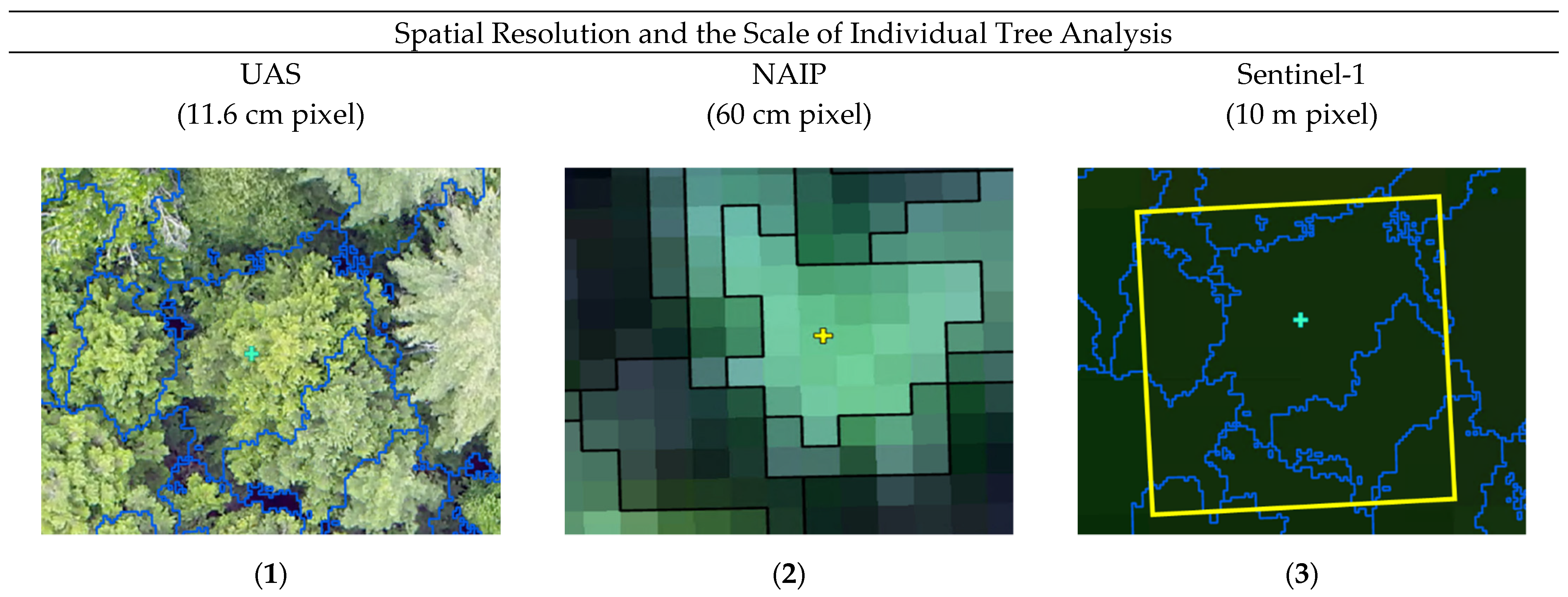
Despite the successes that this research and similar studies have found in the application of UAS for fine scale forest health monitoring, there are several sources of uncertainty that should be further explored. Due to the variability in response that individual trees exhibit to stress, disease, or pests, other researchers have regarded UAS as serving only as a predictor of areas requiring priority management [121]. Even using a binary classification of ‘healthy’ or ‘degraded’ trees, many environmental factors in natural ecosystems may have adversely affected our ‘healthy’ reference trees. While methods do exist to collect field-based spectral reflectance data, which could provide a more direct comparison to UAS remotely sensed image features, these methods elicit considerable time and resources for large study areas; especially in complex, mixed-species forests [122,123,124,125]. Another source of uncertainty in this study was the reliance on the Parrot Sequoia+ multispectral sensor. Despite the sunshine sensor and calibration plate coupled with the Parrot Sequoia+, this sensor is subject to influences of the camera temperature, atmospheric conditions, and variability in the sunshine sensor orientation during flight [126]. Prior to use for normalizing the irradiance of the multispectral images, the sunshine sensor data should be smoothed. This pre-processing would create a more radiometrically consistent estimate of reflectance across flights and especially across study areas [44,126,127]. In the original investigations of this research, we also proposed a comparison to satellite sensors with a higher spectral resolution (e.g., Sentinel-2), as a way to more fully understand the spectral properties of these forest health classes. Early on in the classification, however, it became clear that such satellite sensors lacked the spatial resolution to sufficiently address our reference trees. Figure 5 provides representation of these data sources and the scale of the individual tree observations.
Instead of a comparison between UAS and other remote sensing platforms, data fusion remains a promising expectation for future research with these complex forests. The constraints of frequent monitoring make piloted aircraft techniques logistically challenging [58]. Image fusion allows users to overcome the shortcomings of single data source limitations. For example, with the fusion of satellite and UAS imagery, users could overcome the low spatial resolution of most satellite sensors and the limited coverage that can be accomplished by UAS [57,59]. Lastly, using UAS as an intermediate step for ground-level observations could also increase the efficiencies found in data scaling [72,120]. UAS, as opposed to field measurements, allow for a far greater abundance of reference measurements to be made for scaling models [71]. These imagery combinations may help monitor fine scale change patterns over diverse ecosystems [128]. To accurately engage methods of data fusion between UAS and other sensors, several challenges should be examined. The first being spectral intercalibration. Despite independent radiometric calibration of the UAS data, there can remain differences between the spectral values measured by the UAS and satellite data [59]. Another fundamental challenge is the co-registration of such high-resolution imagery. Events with real-time kinematic (RTK) receivers on the misalignment of either data source by mere pixels could have a dramatic impact on the accuracy of their resulting data product [44,71,128]. Lastly, there is a consequential challenge in collecting imagery from both data sources on the same date. Even with only a few days of separation between collecting such UAS and satellite images, differences in spectral reflectance, solar/viewing angles, or environmental conditions could cause inconsistencies in the data fusion process [57,128]. Another limitation of this study is the rigid and coarse temporal resolution of the airborne imagery. While attempts could be made to align the collection of the field assessments and the UAS imagery for proper comparison, the NAIP imagery is only collected and distributed every couple of years, and may not have been collected during a season in which analyzing a variety of forest disturbances is possible. Future research could benefit from more closely matching the collection field, airborne, and UAS data, as well as the response of individual trees to forest disturbance.

5. Conclusions

The distribution and severity of forest health stressors present too great of an impact on natural ecosystems for field-based monitoring to capture and monitor alone. These events are causing billions of dollars in diminished ecosystem services and management costs across a variety of keystone tree species. Unmanned aerial systems (UAS) provide forest and natural resource managers with the ability to evaluate and monitor individual trees across scales that are consistent with their silvicultural practices. In our study, we examined the viability of UAS for classifying various levels of forest health within complex, mixed-species forests in New England. This assessment of UAS image analysis was completed by making the comparison of these UAS multispectral imagery to multi-factor assessments of crown vigor in the field. These results serve as a basis for prioritizing field investigations of stands identified to consist of stressed or degraded trees throughout mixed-species forests. Using a composite of natural color and multispectral UAS imagery, we achieved overall classification accuracies ranging between 65.43% and 71.19%. Some limitations in our approach include the imprecise calibration of our multispectral imagery and the variation on characteristics found among ‘healthy’ trees in natural environments. A necessary next step for this research is the fusion, rather than comparison, of these UAS with more widely available remotely sensed imagery. Such a step would expand the operational feasibility of UAS and address many of the challenges in precision forest health monitoring and management.

Author Contributions

Conceptualization, B.T.F. and R.G.C.; Methodology, B.T.F.; Supervision, R.G.C.; Resources, R.G.C.; Formal analysis, B.T.F.; Writing—original draft, B.T.F.; Writing—review and editing, R.G.C.; Project administration, R.G.C. All authors have read and agreed to the published version of the manuscript.

Funding

Partial funding was provided by the New Hampshire Agricultural Experiment Station. This is scientific contribution number #2916. This work was supported by the USDA National Institute of Food and Agriculture McIntire Stennis, project #NH00095-M (Accession #1015520).

Institutional Review Board Statement

Not Applicable.

Informed Consent Statement

Not Applicable.

Data Availability Statement

Not Applicable.

Acknowledgments

These analyses utilized processing within Agisoft MetaShape Software Packages with statistical outputs generated from their results. All UAS operations were conducted on University of New Hampshire woodland or partnered properties with permission from local authorities and under the direct supervision of pilots holding Part 107 Remote Pilot in Command licenses. The authors would like to acknowledge Jacob Dearborn, Hannah Stewart, and Richard Hallett for their assistance.

Conflicts of Interest

The authors declare no conflict of interest.

Appendix A

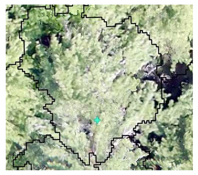
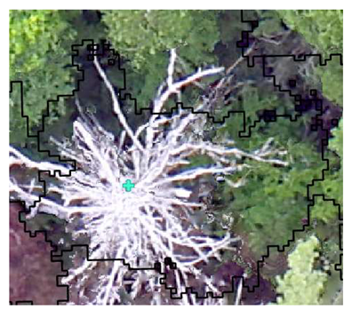
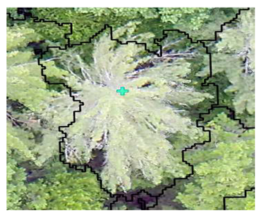
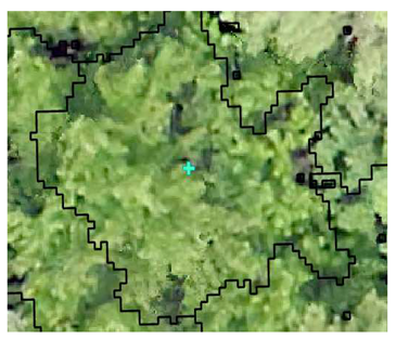
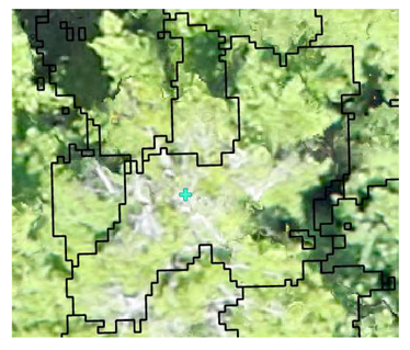
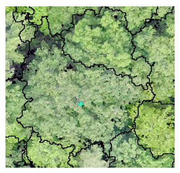
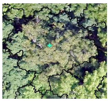
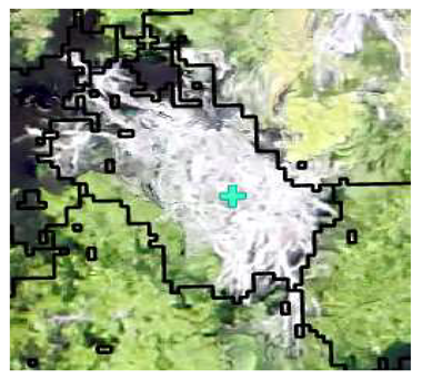
Table A1. Reference samples collected for forest health survey classes using both field methods and photo interpretation. Both coniferous and deciduous trees of the ‘Healthy’, ‘Stressed’, and ‘Dead/Degraded’ classes collected as reference data using both sampling methods are provided as a guide to their similarity.
HealthyStressedDead
Conifer: Field Survey Remotesensing 13 04873 i001
SI = 2
Remotesensing 13 04873 i002
SI = 7
Remotesensing 13 04873 i003
SI = 10
Conifer: Photo
Interpretation
Remotesensing 13 04873 i004 Remotesensing 13 04873 i005 Remotesensing 13 04873 i006
Deciduous: Field Survey Remotesensing 13 04873 i007
SI = 2
Remotesensing 13 04873 i008
SI = 6
Remotesensing 13 04873 i009
SI = 10
Deciduous: Photo
Interpretation
Remotesensing 13 04873 i010 Remotesensing 13 04873 i011 Remotesensing 13 04873 i012
Table A2. Image object features created using eCognition for the purpose of forest health classification using (1) UAS and (2) NAIP segmented imagery.
Image Classification Features
GeometricTextureSpectral
Area (Pixels)
Asymmetry
Border Index
Border Length
Compactness
Density
Length\Width
Radius of Long Ellipsoid
Radius of Short Ellipsoid
Shape Index


UAS Only
GLCM Contrast
GLCM Correlation
GLCM Dissimilarity
GLCM Entropy
GLCM Mean
GLDV Entropy
GLDV Mean
GLDV Contrast
Brightness
Greenness Index
Mean red (SODA\NAIP)
Mean green (SODA\NAIP)
Mean blue (SODA\NAIP)
Mean green (Sequoia)
Mean red (Sequoia)
Mean NIR (Sequoia\NAIP)
Mean red edge (Sequoia)
NDVI
NGRDI
Std. Dev. red (SODA\NAIP)
Std. Dev. green (SODA\NAIP)
Std. Dev. blue (SODA\NAIP)
Std. Dev. green (Sequoia)
Std. Dev. red (Sequoia)
Std. Dev. NIR (Sequoia\NAIP)
Std. Dev. red edge (Sequoia)

References

  1. Oliver, C.D.; Larson, B.A. Forest Stand Dynamics, Updated ed.; John Wiley & Sons: New York, NY, USA, 1996. [Google Scholar]
  2. Frolking, S.; Palace, M.W.; Clark, D.B.; Chambers, J.Q.; Shugart, H.H.; Hurtt, G.C. Forest disturbance and recovery: A general review in the context of spaceborne remote sensing of impacts on aboveground biomass and canopy structure. J. Geophys. Res. Biogeosciences 2009, 114, G00E02. [Google Scholar] [CrossRef]
  3. Coleman, T.W.; Graves, A.D.; Heath, Z.; Flowers, R.W.; Hanavan, R.P.; Cluck, D.R.; Ryerson, D. Accuracy of aerial detection surveys for mapping insect and disease disturbances in the United States. For. Ecol. Manag. 2018, 430, 321–336. [Google Scholar] [CrossRef]
  4. Wilson, D.C.; Morin, R.S.; Frelich, L.E.; Ek, A.R. Monitoring disturbance intervals in forests: A case study of increasing forest disturbance in Minnesota. Ann. For. Sci. 2019, 76, 78. [Google Scholar] [CrossRef]
  5. Aukema, J.E.; Leung, B.; Kovacs, K.; Chivers, C.; Britton, K.O.; Englin, J.; Frankel, S.J.; Haight, R.G.; Holmes, T.P.; Liebhold, A.M.; et al. Economic impacts of Non-Native forest insects in the continental United States. PLoS ONE 2011, 6, e24587. [Google Scholar] [CrossRef]
  6. Pontius, J.; Hanavan, R.P.; Hallett, R.A.; Cook, B.D.; Corp, L.A. High spatial resolution spectral unmixing for mapping ash species across a complex urban environment. Remote Sens. Environ. 2017, 199, 360–369. [Google Scholar] [CrossRef]
  7. Hassaan, O.; Nasir, A.K.; Roth, H.; Khan, M.F. Precision Forestry: Trees Counting in Urban Areas Using Visible Imagery based on an Unmanned Aerial Vehicle. IFAC PapersOnLine 2016, 49, 16–21. [Google Scholar] [CrossRef]
  8. Lausch, A.; Erasmi, S.; King, D.J.; Magdon, P.; Heurich, M. Understanding forest health with Remote sensing—Part II—A review of approaches and data models. Remote Sens. 2017, 9, 129. [Google Scholar] [CrossRef] [Green Version]
  9. Lausch, A.; Erasmi, S.; King, D.J.; Magdon, P.; Heurich, M. Understanding forest health with remote sensing—Part I—A review of spectral traits, processes and remote-sensing characteristics. Remote Sens. 2016, 8, 1029. [Google Scholar] [CrossRef] [Green Version]
  10. Kopinga, J.; Van Den Burg, J. Using Soil and Foliar Analysis to Diagnose the Nutritional Status of Urban Trees. J. Arboric. 1995, 21, 17–24. [Google Scholar]
  11. Pan, Y.; McCullough, K.; Hollinger, D.Y. Forest biodiversity, relationships to structural and functional attributes, and stability in New England forests. For. Ecosyst. 2018, 5, 14. [Google Scholar] [CrossRef] [Green Version]
  12. Gerhards, M.; Schlerf, M.; Mallick, K.; Udelhoven, T. Challenges and future perspectives of multi-/Hyperspectral thermal infrared remote sensing for crop water-stress detection: A review. Remote Sens. 2019, 11, 1240. [Google Scholar] [CrossRef] [Green Version]
  13. Ward, K.T.; Johnson, G.R. Geospatial methods provide timely and comprehensive urban forest information. Urban For. Urban Green. 2007, 6, 15–22. [Google Scholar] [CrossRef]
  14. Steinman, J. Forest Health Monitoring in the North-Eastern United States: Disturbances and Conditions During 1993–2002; Tech. Pap. NA-01-04; U.S. Department of Agriculture, Forest Service, State and Private Forestry, Northeastern Area: Newtown Square, PA, USA, 2004; 46p.
  15. McLaughlin, S.; Percy, K. Forest health in North America: Some perspectives on actual and potential roles of climate and air pollution. Water Air Soil Pollut. 1999, 116, 151–197. [Google Scholar] [CrossRef]
  16. Meng, J.; Li, S.; Wang, W.; Liu, Q.; Xie, S.; Ma, W. Mapping forest health using spectral and textural information extracted from SPOT-5 satellite images. Remote Sens. 2016, 8, 719. [Google Scholar] [CrossRef] [Green Version]
  17. Broders, K.; Munck, I.; Wyka, S.; Iriarte, G.; Beaudoin, E. Characterization of fungal pathogens associated with white pine needle damage (WPND) in Northeastern North America. Forests 2015, 6, 4088–4104. [Google Scholar] [CrossRef]
  18. Wyka, S.A.; Smith, C.; Munck, I.A.; Rock, B.N.; Ziniti, B.L.; Broders, K. Emergence of white pine needle damage in the northeastern United States is associated with changes in pathogen pressure in response to climate change. Glob. Chang. Biol. 2017, 23, 394–405. [Google Scholar] [CrossRef]
  19. Poland, T.M.; McCullough, D.G. Emerald ash borer: Invasion of the urban forest and the threat to North America’s ash resource. J. For. 2006, 104, 118–124. [Google Scholar]
  20. Pasquarella, V.J.; Elkinton, J.S.; Bradley, B.A. Extensive gypsy moth defoliation in Southern New England characterized using Landsat satellite observations. Biol. Invasions 2018, 20, 3047–3053. [Google Scholar] [CrossRef]
  21. Orwig, D.A.; Foster, D.R. Forest Response to the Introduced Hemlock Woolly Adelgid in Southern New England, USA. J. Torrey Bot. Soc. 1998, 125, 60–73. [Google Scholar] [CrossRef]
  22. Simoes, J.; Markowski-Lindsay, M.; Butler, B.J.; Kittredge, D.B.; Thompson, J.; Orwig, D. Assessing New England family forest owners’ invasive insect awareness. J. Ext. 2019, 57, 16. [Google Scholar]
  23. Burns, R.M.; Honkala, B.H. Silvics of North America; Agriculture Handbook 654; United States Department of Agriculture, Forest Service: Washington, DC, USA, 1990; Volume 2, p. 877.
  24. McCune, B. Lichen Communities as Indicators of Forest Health. Bryologist 2000, 103, 353–356. [Google Scholar] [CrossRef]
  25. Pause, M.; Schweitzer, C.; Rosenthal, M.; Keuck, V.; Bumberger, J.; Dietrich, P.; Heurich, M.; Jung, A.; Lausch, A. In situ/remote sensing integration to assess forest health—A review. Remote Sens. 2016, 8, 471. [Google Scholar] [CrossRef] [Green Version]
  26. Tucker, C.J.; Townshend, J.R.G.; Goff, T.E. African land-cover classification using satellite data. Science 1985, 227, 369–375. [Google Scholar] [CrossRef] [PubMed]
  27. Goetz, S.; Dubayah, R. Advances in remote sensing technology and implications for measuring and monitoring forest carbon stocks and change. Carbon Manag. 2011, 2, 231–244. [Google Scholar] [CrossRef]
  28. Zaman, B.; Jensen, A.M.; McKee, M. Use of high-resolution multispectral imagery acquired with an autonomous unmanned aerial vehicle to quantify the spread of an invasive wetlands species. In Proceedings of the 2011 IEEE International Geoscience and Remote Sensing Symposium, IEEE, Vancouver, BC, Canada, 24–29 July 2011; pp. 803–806. [Google Scholar]
  29. Innes, J.L. An assessment of the use of crown structure for the determination of the health of beech (Fagus sylvatica). Forestry 1998, 71, 113–130. [Google Scholar] [CrossRef] [Green Version]
  30. Pontius, J.; Hallett, R. Comprehensive Methods for Earlier Detection and Monitoring of Forest Decline. For. Sci. 2014, 60, 1156–1163. [Google Scholar] [CrossRef]
  31. Hallett, R.; Johnson, M.L.; Sonti, N.F. Assessing the tree health impacts of salt water flooding in coastal cities: A case study in New York City. Landsc. Urban Plan. 2018, 177, 171–177. [Google Scholar] [CrossRef]
  32. Hallett, R.A.; Bailey, S.W.; Horsley, S.B.; Long, R.P. Influence of nutrition and stress on sugar maple at a regional scale. Can. J. For. Res. 2006, 36, 2235–2246. [Google Scholar] [CrossRef]
  33. HTHC. Healthy Trees Healthy Cities. Available online: https://healthytreeshealthycitiesapp.org/ (accessed on 1 August 2021).
  34. Guidi, L.; Lo Piccolo, E.; Landi, M. Chlorophyll fluorescence, photoinhibition and abiotic stress: Does it make any difference the fact to be a C3 or C4 species? Front. Plant Sci. 2019, 10, 174. [Google Scholar] [CrossRef]
  35. Gatica-Saavedra, P.; Echeverría, C.; Nelson, C.R. Ecological indicators for assessing ecological success of forest restoration: A world review. Restor. Ecol. 2017, 25, 850–857. [Google Scholar] [CrossRef]
  36. Noss, R.F. Assessing and monitoring forest biodiversity: A suggested framework and indicators. For. Ecol. Manag. 1999, 115, 135–146. [Google Scholar] [CrossRef]
  37. Lindenmayer, D.B.; Margules, C.R.; Botkin, D.B. Indicators of Biodiversity for Ecologically Sustainable Forest Management. Conserv. Biol. 2000, 14, 941–950. [Google Scholar] [CrossRef]
  38. Juutinen, A.; Mönkkönen, M. Testing alternative indicators for biodiversity conservation in old-growth boreal forests: Ecology and economics. Ecol. Econ. 2004, 50, 35–48. [Google Scholar] [CrossRef]
  39. Schrader-Patton, C.; Grulke, N.; Bienz, C. Assessment of ponderosa pine vigor using four-band aerial imagery in south central oregon: Crown objects to landscapes. Forests 2021, 12, 612. [Google Scholar] [CrossRef]
  40. Grulke, N.; Bienz, C.; Hrinkevich, K.; Maxfield, J.; Uyeda, K. Quantitative and qualitative approaches to assess tree vigor and stand health in dry pine forests. For. Ecol. Manag. 2020, 465, 118085. [Google Scholar] [CrossRef]
  41. Royle, D.D.; Lathrop, R.G. Monitoring Hemlock Forest Health in New Jersey Using Landsat TM Data and Change Detection Techniques. For. Sci. 1997, 49, 9. [Google Scholar]
  42. Bigler, C.; Vitasse, Y. Premature leaf discoloration of European deciduous trees is caused by drought and heat in late spring and cold spells in early fall. Agric. For. Meteorol. 2021, 307, 108492. [Google Scholar] [CrossRef]
  43. Hoffbeck, J.P.; Landgrebe, D.A. Classification of Remote Sensing Images Having High Spectral Resolution. Remote Sens. Environ. 1996, 57, 119–126. [Google Scholar] [CrossRef]
  44. Jensen, J. Introductory Digital Image Processing: A Remote Sensing Perspective, 4th ed.; Pearson Education Inc.: Glenview, IL, USA, 2016. [Google Scholar]
  45. Horsley, S.B.; Long, R.P.; Bailey, S.W.; Hallett, R.A.; Wargo, P.M. Health of Eastern North American sugar maple forests and factors affecting decline. North. J. Appl. For. 2002, 19, 34–44. [Google Scholar] [CrossRef]
  46. Gago, J.; Douthe, C.; Coopman, R.E.; Gallego, P.P.; Ribas-Carbo, M.; Flexas, J.; Escalona, J.; Medrano, H. UAVs challenge to assess water stress for sustainable agriculture. Agric. Water Manag. 2015, 153, 9–19. [Google Scholar] [CrossRef]
  47. Chaerle, L.; Van Der Straeten, D. Imaging Techniques and the early detection of plant stress. Trends Plant Sci. 2000, 5, 495–501. [Google Scholar] [CrossRef]
  48. Näsi, R.; Honkavaara, E.; Tuominen, S.; Saari, H.; Pölönen, I.; Hakala, T.; Viljanen, N.; Soukkamäki, J.; Näkki, I.; Ojanen, H.; et al. UAS based tree species identification using the novel FPI based hyperspectral cameras in visible, NIR and SWIR spectral ranges. In International Archives of the Photogrammetry, Remote Sensing and Spatial Information Sciences, Proceedings of the XXIII ISPRS Congress, Prague, Czech Republic, 12–19 July 2016; International Society for Photogrammetry and Remote Sensing: Istanbul, Turkey, 2016; pp. 1143–1148. [Google Scholar] [CrossRef]
  49. Choi, S.; Kim, Y.; Lee, J.H.; You, H.; Jang, B.J.; Jung, K.H. Minimizing Device-to-Device Variation in the Spectral Response of Portable Spectrometers. J. Sens. 2019, 2019, 8392583. [Google Scholar] [CrossRef] [Green Version]
  50. Lu, B.; He, Y.; Liu, H.H.T. Mapping vegetation biophysical and biochemical properties using unmanned aerial vehicles-acquired imagery. Int. J. Remote Sens. 2018, 39, 15–16. [Google Scholar] [CrossRef]
  51. Kerr, J.T.; Ostrovsky, M. From space to species: Ecological applications for remote sensing. Trends Ecol. Evol. 2003, 18, 299–305. [Google Scholar] [CrossRef]
  52. Goodbody, T.R.H.; Coops, N.C.; Hermosilla, T.; Tompalski, P.; Crawford, P. Assessing the status of forest regeneration using digital aerial photogrammetry and unmanned aerial systems. Int. J. Remote Sens. 2018, 39, 5246–5264. [Google Scholar] [CrossRef]
  53. Otsu, K.; Pla, M.; Duane, A.; Cardil, A.; Brotons, L. Estimating the threshold of detection on tree crown defoliation using vegetation indices from UAS multispectral imagery. Drones 2019, 3, 80. [Google Scholar] [CrossRef] [Green Version]
  54. Zhang, X.; Qiu, F.; Zhan, C.; Zhang, Q.; Li, Z.; Wu, Y.; Huang, Y.; Chen, X. Acquisitions and applications of forest canopy hyperspectral imageries at hotspot and multiview angle using unmanned aerial vehicle platform. J. Appl. Remote Sens. 2020, 14, 1. [Google Scholar] [CrossRef]
  55. Liu, L.; Coops, N.C.; Aven, N.W.; Pang, Y. Mapping urban tree species using integrated airborne hyperspectral and LiDAR remote sensing data. Remote Sens. Environ. 2017, 200, 170–182. [Google Scholar] [CrossRef]
  56. Zhao, D.; Pang, Y.; Liu, L.; Li, Z. Individual tree classification using airborne LiDAR and hyperspectral data in a natural mixed forest of northeast China. Forests 2020, 11, 303. [Google Scholar] [CrossRef] [Green Version]
  57. Jenerowicz, A.; Siok, K.; Woroszkiewicz, M.; Orych, A. The fusion of satellite and UAV data: Simulation of high spatial resolution band. In Remote Sensing for Agriculture, Ecosystems, and Hydrology XIX, Proceedings of the SPIE Remote Sensing, Warsaw, Poland, 11–14 September 2017; International Society for Optics and Photonics: Bellingham, WA, USA, 2017; Volume 10421, p. 104211. [Google Scholar] [CrossRef]
  58. Berra, E.F.; Gaulton, R.; Barr, S. Assessing spring phenology of a temperate woodland: A multiscale comparison of ground, unmanned aerial vehicle and Landsat satellite observations. Remote Sens. Environ. 2019, 223, 229–242. [Google Scholar] [CrossRef]
  59. Alvarez-Vanhard, E.; Houet, T.; Mony, C.; Lecoq, L.; Corpetti, T. Can UAVs fill the gap between in situ surveys and satellites for habitat mapping? Remote Sens. Environ. 2020, 243, 111780. [Google Scholar] [CrossRef]
  60. Næsset, E.; Gobakken, T.; McRoberts, R.E. A model-dependent method for monitoring subtle changes in vegetation height in the boreal-alpine ecotone using bi-temporal, three dimensional point data from airborne laser scanning. Remote Sens. 2019, 11, 1804. [Google Scholar] [CrossRef] [Green Version]
  61. Marshall, D.M.; Barnhart, R.K.; Shappee, E.; Most, M. Introduction to Unmanned Aerial Systems, 2nd ed.; CRC Press: Boca Raton, FL, USA, 2016. [Google Scholar]
  62. Fraser, B.T.; Congalton, R.G. Issues in Unmanned Aerial Systems (UAS) data collection of complex forest environments. Remote Sens. 2018, 10, 908. [Google Scholar] [CrossRef] [Green Version]
  63. Lelong, C.C.D.; Burger, P.; Jubelin, G.; Roux, B.; Labbé, S.; Baret, F. Assessment of unmanned aerial vehicles imagery for quantitative monitoring of wheat crop in small plots. Sensors 2008, 8, 3557–3585. [Google Scholar] [CrossRef]
  64. Gini, R.; Passoni, D.; Pinto, L.; Sona, G. Use of unmanned aerial systems for multispectral survey and tree classification: A test in a park area of northern Italy. Eur. J. Remote Sens. 2014, 47, 251–269. [Google Scholar] [CrossRef]
  65. Lehmann, J.R.K.; Nieberding, F.; Prinz, T.; Knoth, C. Analysis of unmanned aerial system-based CIR images in forestry—A new perspective to monitor pest infestation levels. Forests 2015, 6, 594–612. [Google Scholar] [CrossRef] [Green Version]
  66. Michez, A.; Piégay, H.; Lisein, J.; Claessens, H.; Lejeune, P. Classification of riparian forest species and health condition using multi-temporal and hyperspatial imagery from unmanned aerial system. Environ. Monit. Assess. 2016, 188, 146. [Google Scholar] [CrossRef] [PubMed] [Green Version]
  67. Zhou, X.; Zhang, X. Individual tree parameters estimation for plantation forests based on UAV oblique photography. IEEE Access 2020, 8, 96184–96198. [Google Scholar] [CrossRef]
  68. Liang, X.; Wang, Y.; Pyörälä, J.; Lehtomäki, M.; Yu, X.; Kaartinen, H.; Kukko, A.; Honkavaara, E.; Issaoui, A.E.I.; Nevalainen, O.; et al. Forest in situ observations using unmanned aerial vehicle as an alternative of terrestrial measurements. For. Ecosyst. 2019, 6, 20. [Google Scholar] [CrossRef] [Green Version]
  69. Tang, L.; Shao, G. Drone remote sensing for forestry research and practices. J. For. Res. 2015, 26, 791–797. [Google Scholar] [CrossRef]
  70. Smigaj, M.; Gaulton, R.; Suárez, J.C.; Barr, S.L. Canopy temperature from an Unmanned Aerial Vehicle as an indicator of tree stress associated with red band needle blight severity. For. Ecol. Manag. 2019, 433, 699–708. [Google Scholar] [CrossRef]
  71. Kattenborn, T.; Lopatin, J.; Förster, M.; Braun, A.C.; Fassnacht, F.E. UAV data as alternative to field sampling to map woody invasive species based on combined Sentinel-1 and Sentinel-2 data. Remote Sens. Environ. 2019, 227, 61–73. [Google Scholar] [CrossRef]
  72. Revill, A.; Florence, A.; Macarthur, A.; Hoad, S.; Rees, R.; Williams, M. Quantifying uncertainty and bridging the scaling gap in the retrieval of leaf area index by coupling sentinel-2 and UAV observations. Remote Sens. 2020, 12, 1843. [Google Scholar] [CrossRef]
  73. Janowiak, M.K.; D’Amato, A.W.; Swanston, C.W.; Iverson, L.; Thompson, F.R.; Dijak, W.D.; Matthews, S.; Peters, M.P.; Prasad, A.; Fraser, J.S.; et al. New England and Northern New York Forest Ecosystem Vulnerability Assessment and Synthesis: A Report from the New England Climate Change Response Framework Project; NRS-173; U.S. Department of Agriculture, Forest Service, Northern Research Station: Newtown Square, PA, USA, 2018; p. 234. [CrossRef]
  74. University of New Hampshire Office of Woodlands and Natural Areas. Available online: https://colsa.unh.edu/woodlands (accessed on 1 September 2021).
  75. Eisenhaure, S. Kingman Farm. Management and Operations Plan; University of New Hampshire, Office of Woodlands and Natural Areas: Durham, NH, USA, 2018. [Google Scholar]
  76. Fraser, B.T.; Congalton, R.G. Estimating Primary Forest Attributes and Rare Community Charecteristics using Unmanned Aerial Systems (UAS): An Enrichment of Conventional Forest Inventories. Remote Sens. 2021, 13, 2971. [Google Scholar] [CrossRef]
  77. EOS. Arrow 200 RTK GNSS. Available online: https://eos-gnss.com/product/arrow-series/arrow-200/?gclid=Cj0KCQjw2tCGBhCLARIsABJGmZ47-nIPNrAuu7Xobgf3P0HGlV4mMLHHWZz25lyHM6UuI_pPCu7b2gMaAukeEALw_wcB (accessed on 1 August 2021).
  78. Hallett, R.; Hallett, T. Citizen Science and Tree Health Assessment: How useful are the data? Arboric. Urban For. 2018, 44, 236–247. [Google Scholar] [CrossRef]
  79. Green, R. Sampling Design and Statistical Methods for Environmental Biologists; John Wiley and Sons Inc.: New York, NY, USA, 1979. [Google Scholar]
  80. USDA. NAIP Imagery. Available online: https://www.fsa.usda.gov/programs-and-services/aerial-photography/imagery-programs/naip-imagery/ (accessed on 1 September 2021).
  81. Fraser, B.; Congalton, R.G. A Comparison of Methods for Determining Forest Composition from High-Spatial Resolution Remotely Sensed Imagery. Forests 2021, 12, 1290. [Google Scholar] [CrossRef]
  82. Louhaichi, M.; Borman, M.M.; Johnson, D.E. Spatially located platform and aerial photography for documentation of grazing impacts on wheat. Geocarto Int. 2001, 16, 65–70. [Google Scholar] [CrossRef]
  83. SenseFly. eBee Plus Drone User Manual v1.8; senseFly Parrot Group: Lausanne, Switzerland, 2018; p. 107. [Google Scholar]
  84. SenseFly. eBee X Drone User Manual v1.3; senseFly Parrot Group: Lausanne, Switzerland, 2019; p. 96. [Google Scholar]
  85. SenseFly. senseFly S.O.D.A. Photogrammetry Camera. Available online: https://www.sensefly.com/camera/sensefly-soda-photogrammetry-camera/ (accessed on 1 September 2021).
  86. SenseFly. senseFly Aeria X Photogrammetry Camera. Available online: https://www.sensefly.com/camera/sensefly-aeria-x-photogrammetry-camera/ (accessed on 1 September 2021).
  87. SenseFly. Parrot Sequoia+ Multispectral Camera. Available online: https://www.sensefly.com/camera/parrot-sequoia/ (accessed on 1 September 2021).
  88. SenseFly. eMotion Drone Flight Management Software Versions 3.15 (eBee Plus) and 3.19 (eBee X). Available online: https://www.sensefly.com/software/emotion/ (accessed on 1 October 2021).
  89. Puliti, S.; Ørka, H.O.; Gobakken, T.; Næsset, E. Inventory of small forest areas using an unmanned aerial system. Remote Sens. 2015, 7, 9632–9654. [Google Scholar] [CrossRef] [Green Version]
  90. Dandois, J.P.; Olano, M.; Ellis, E.C. Optimal altitude, overlap, and weather conditions for computer vision UAV estimates of forest structure. Remote Sens. 2015, 7, 13895–13920. [Google Scholar] [CrossRef] [Green Version]
  91. National Oceanic and Atmospheric Administration. Continuously Operating Reference Stations (CORS); National Oceanic and Atmospheric Administration. Available online: https://geodesy.noaa.gov/CORS/ (accessed on 1 October 2021).
  92. Gu, J.; Grybas, H.; Congalton, R.G. A comparison of forest tree crown delineation from unmanned aerial imagery using canopy height models vs. spectral lightness. Forests 2020, 11, 605. [Google Scholar] [CrossRef]
  93. Chen, Y.; Ming, D.; Zhao, L.; Lv, B.; Zhou, K.; Qing, Y. Review on high spatial resolution remote sensing image segmentation evaluation. Photogramm. Eng. Remote Sens. 2018, 84, 629–646. [Google Scholar] [CrossRef]
  94. GRANIT. GRANIT LiDAR Distribution Site. Available online: https://lidar.unh.edu/map/ (accessed on 1 October 2021).
  95. Panagiotidis, D.; Abdollahnejad, A.; Surový, P.; Chiteculo, V. Determining tree height and crown diameter from high-resolution UAV imagery. Int. J. Remote Sens. 2017, 38, 2392–2410. [Google Scholar] [CrossRef]
  96. Gu, J.; Congalton, R.G. Individual Tree Crown Delineation from UAS Imagery Based on Region Growing by Over-Segments With a Competitive Mechanism. IEEE Trans. Geosci. Remote Sens. 2021, 1–11. [Google Scholar] [CrossRef]
  97. Alonzo, M.; Bookhagen, B.; Roberts, D.A. Urban tree species mapping using hyperspectral and lidar data fusion. Remote Sens. Environ. 2014, 148, 70–83. [Google Scholar] [CrossRef]
  98. Hogland, J.; Anderson, N.; St Peter, J.; Drake, J.; Medley, P. Mapping Forest Characteristics at Fine Resolution across Large Landscapes of the Southeastern United States Using NAIP Imagery and FIA Field Plot Data. ISPRS Int. J. Geo Inf. 2018, 7, 140. [Google Scholar] [CrossRef] [Green Version]
  99. Chandel, A.K.; Molaei, B.; Khot, L.R.; Peters, R.T.; Stöckle, C.O. High resolution geospatial evapotranspiration mapping of irrigated field crops using multispectral and thermal infrared imagery with metric energy balance model. Drones 2020, 4, 52. [Google Scholar] [CrossRef]
  100. García, M.; Saatchi, S.; Ustin, S.; Balzter, H. Modelling forest canopy height by integrating airborne LiDAR samples with satellite Radar and multispectral imagery. Int. J. Appl. Earth Obs. Geoinf. 2018, 66, 159–173. [Google Scholar] [CrossRef]
  101. Congalton, R.G.; Green, K. Assessing the Accuracy of Remotely Sensed Data: Principals and Practices, 3rd ed.; CRC Press: Boca Raton, FL, USA, 2019. [Google Scholar]
  102. Pedregosa, F.; Varoquaux, G.; Gramfort, A.; Michel, V.; Thirion, B.; Grisel, O.; Blondel, M.; Prettenhofer, P.; Weiss, R.; Dubourg, V.; et al. Scikit-learn: Machine Learning in Python. J. Mach. Learn. Res. 2011, 12, 2825–2830. [Google Scholar]
  103. Breiman, L. Random Forests. Mach. Learn. 2001, 45, 5–32. [Google Scholar] [CrossRef] [Green Version]
  104. Maxwell, A.E.; Warner, T.A.; Fang, F. Implementation of machine-learning classification in remote sensing: An applied review. Int. J. Remote Sens. 2018, 39, 2784–2817. [Google Scholar] [CrossRef] [Green Version]
  105. Pal, M.; Mather, P.M. Support vector machines for classification in remote sensing. Int. J. Remote Sens. 2005, 26, 1007–1011. [Google Scholar] [CrossRef]
  106. Chapelle, O.; Haffner, P.; Vapnik, V.N. Support vector machines for histogram-based image classification. IEEE Trans. Neural Netw. 1999, 10, 1055–1064. [Google Scholar] [CrossRef]
  107. Wessel, M.; Brandmeier, M.; Tiede, D. Evaluation of different machine learning algorithms for scalable classification of tree types and tree species based on Sentinel-2 data. Remote Sens. 2018, 10, 1419. [Google Scholar] [CrossRef] [Green Version]
  108. Morin, R.S.; Barnett, C.J.; Butler, B.J.; Crocker, S.J.; Domke, G.M.; Hansen, M.H.; Hatfield, M.A.; Horton, J.; Kurtz, C.M.; Lister, T.W.; et al. Forests of Vermont and New Hampshire 2012; Resource Bulletin NRS-95; U.S. Department of Agriculture United States Forest Service, Northern Research Station: Newtown Square, PA, USA, 2015; p. 80.
  109. Vitousek, P.M.; D’Antonio, C.M.; Loope, L.L.; Westbrooks, R. Biological invasions as global environmental change. Am. Sci. 1996, 84, 468–478. [Google Scholar]
  110. Thompson, I.D.; Guariguata, M.R.; Okabe, K.; Bahamondez, C.; Nasi, R.; Heymell, V.; Sabogal, C. An operational framework for defining and monitoring forest degradation. Ecol. Soc. 2013, 18, 20. [Google Scholar] [CrossRef]
  111. Gunn, J.S.; Ducey, M.J.; Belair, E. Evaluating degradation in a North American temperate forest. For. Ecol. Manag. 2019, 432, 415–426. [Google Scholar] [CrossRef]
  112. Meng, Y.; Cao, B.; Dong, C.; Dong, X. Mount Taishan Forest ecosystem health assessment based on forest inventory data. Forests 2019, 10, 657. [Google Scholar] [CrossRef] [Green Version]
  113. Zhang, L.; Sun, X.; Wu, T.; Zhang, H. An Analysis of Shadow Effects on Spectral Vegetation Indexes Using a Ground-Based Imaging Spectrometer. IEEE Geosci. Remote Sens. Lett. 2015, 12, 2188–2192. [Google Scholar] [CrossRef]
  114. Mulatu, K.A.; Decuyper, M.; Brede, B.; Kooistra, L.; Reiche, J.; Mora, B.; Herold, M. Linking terrestrial LiDAR scanner and conventional forest structure measurements with multi-modal satellite data. Forests 2019, 10, 291. [Google Scholar] [CrossRef] [Green Version]
  115. Liu, K.; Shen, X.; Cao, L.; Wang, G.; Cao, F. Estimating forest structural attributes using UAV-LiDAR data in Ginkgo plantations. ISPRS J. Photogramm. Remote Sens. 2018, 146, 465–482. [Google Scholar] [CrossRef]
  116. Hugenholtz, C.H.; Whitehead, K.; Brown, O.W.; Barchyn, T.E.; Moorman, B.J.; LeClair, A.; Riddell, K.; Hamilton, T. Geomorphological mapping with a small unmanned aircraft system (sUAS): Feature detection and accuracy assessment of a photogrammetrically-derived digital terrain model. Geomorphology 2013, 194, 16–24. [Google Scholar] [CrossRef] [Green Version]
  117. Maxwell, A.E.; Warner, T.A.; Vanderbilt, B.C.; Ramezan, C.A. Land cover classification and feature extraction from National Agriculture Imagery Program (NAIP) Orthoimagery: A review. Photogramm. Eng. Remote Sens. 2017, 83, 737–747. [Google Scholar] [CrossRef]
  118. Näsi, R.; Honkavaara, E.; Blomqvist, M.; Lyytikäinen-Saarenmaa, P.; Hakala, T.; Viljanen, N.; Kantola, T.; Holopainen, M. Remote sensing of bark beetle damage in urban forests at individual tree level using a novel hyperspectral camera from UAV and aircraft. Urban For. Urban Green. 2018, 30, 72–83. [Google Scholar] [CrossRef]
  119. Cardil, A.; Vepakomma, U.; Brotons, L. Assessing pine processionary moth defoliation using unmanned aerial systems. Forests 2017, 8, 402. [Google Scholar] [CrossRef] [Green Version]
  120. Kampen, M.; Lederbauer, S.; Mund, J.P.; Immitzer, M. UAV-Based Multispectral Data for Tree Species Classification and Tree Vitality Analysis. In Proceedings of the Dreilandertagung der DGPF, der OVG und der SGPF, Vienna, Austria, 20–22 February 2019; pp. 623–639. [Google Scholar]
  121. Barbedo, J.G.A. A review on the use of unmanned aerial vehicles and imaging sensors for monitoring and assessing plant stresses. Drones 2019, 3, 40. [Google Scholar] [CrossRef] [Green Version]
  122. Tree, R.M.; Slusser, J. Measurement of spectral signatures of invasive plant species with a low cost spectrometer. In Proceedings of the Optics and Photonics, San Diego, CA, USA, 31 July–4 August 2005; Volume 5886, pp. 264–272. [Google Scholar]
  123. Jha, C.S.; Singhal, J.; Reddy, S.; Rajashekar, G.; Maity, S.; Patnaik, C.; Das, A.; Misra, A.; Singh, C.P.; Mohapatra, J. Characterization of species diversity and forest health using AVIRIS-NG hyperspectral remote sensing data. Curr. Sci. 2019, 116, 1124–1135. [Google Scholar] [CrossRef]
  124. Adam, E.; Deng, H.; Odindi, J.; Abdel-Rahman, E.M.; Mutanga, O. Detecting the early stage of phaeosphaeria leaf spot infestations in maize crop using in situ hyperspectral data and guided regularized random forest algorithm. J. Spectrosc. 2017, 2017, 6961387. [Google Scholar] [CrossRef]
  125. Zhu, X.; Skidmore, A.K.; Darvishzadeh, R.; Wang, T. Estimation of forest leaf water content through inversion of a radiative transfer model from LiDAR and hyperspectral data. Int. J. Appl. Earth Obs. Geoinf. 2019, 74, 120–129. [Google Scholar] [CrossRef]
  126. Olsson, P.O.; Vivekar, A.; Adler, K.; Garcia Millan, V.E.; Koc, A.; Alamrani, M.; Eklundh, L. Radiometric correction of multispectral uas images: Evaluating the accuracy of the parrot sequoia camera and sunshine sensor. Remote Sens. 2021, 13, 577. [Google Scholar] [CrossRef]
  127. Berni, J.A.J.; Zarco-Tejada, P.J.; Suarez, L.; Fereres, E. Thermal and Narrowband Multispectral Remote Sensing for Vegetation Monitoring from an Unmanned Aerial Vehicle. IEEE Trans. Geosci. Remote Sens. 2009, 47, 722–738. [Google Scholar] [CrossRef] [Green Version]
  128. Xia, H.; Zhao, W.; Li, A.; Bian, J.; Zhang, Z. Subpixel inundation mapping using landsat-8 OLI and UAV data for a wetland region on the zoige plateau, China. Remote Sens. 2017, 9, 31. [Google Scholar] [CrossRef] [Green Version]
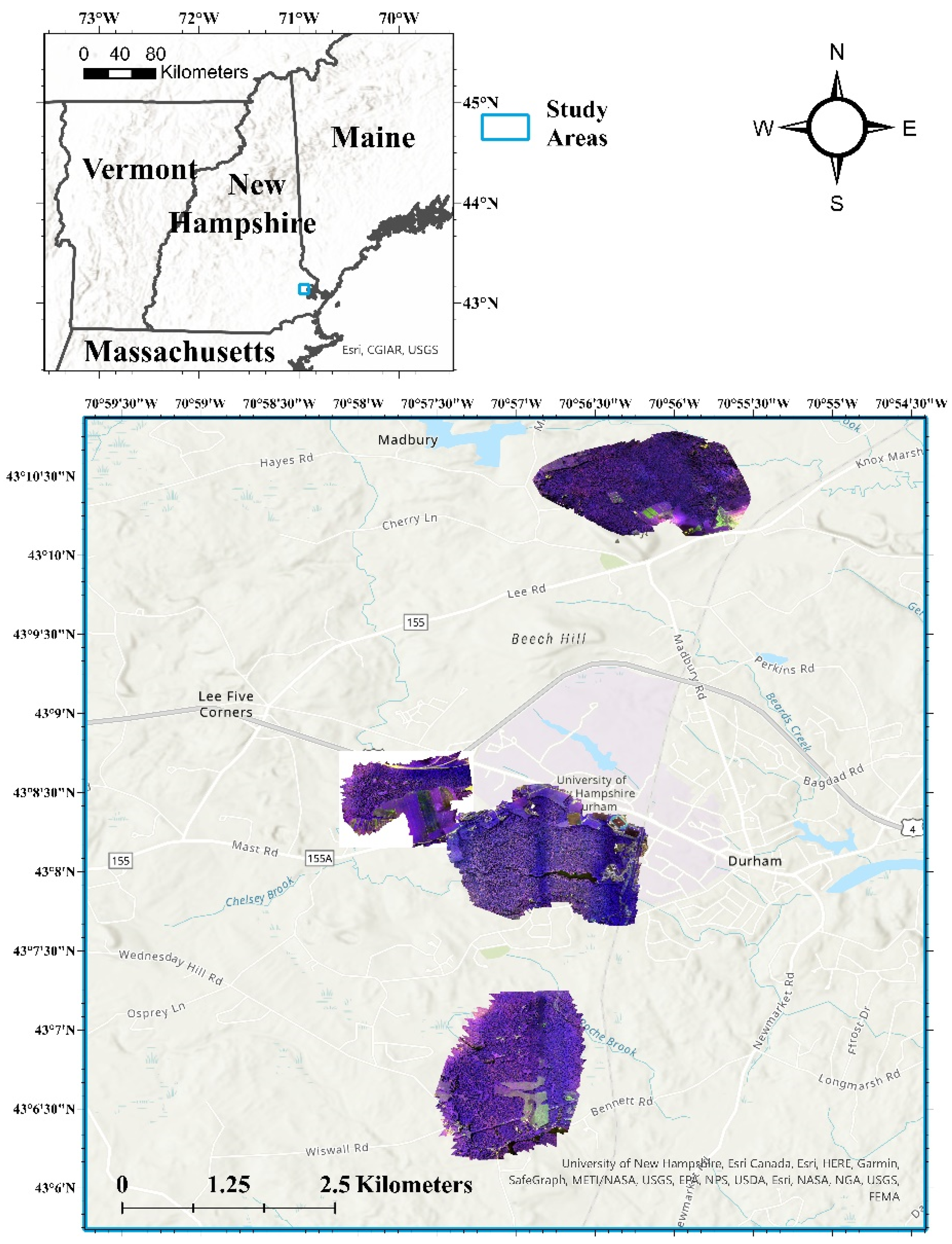
Figure 1. Four woodland properties evaluated during the assessment of forest health. Each property is shown using the multispectral (false color composite) orthoimagery generated from the unmanned aerial system (UAS) imagery.
Remotesensing 13 04873 g001
Figure 2. Mean decrease in impurity (MDI) image feature scores calculated using the NAIP imagery and random forest classifier.
Remotesensing 13 04873 g002
Figure 3. UAS classification feature importance scores calculated using the MDI test.
Remotesensing 13 04873 g003
Figure 4. Example map of stressed trees classified using UAS multispectral imagery.
Remotesensing 13 04873 g004
Figure 5. Characterization of individual trees using three sources of remotely sensed imagery. (1) UAS natural color imagery, segmented to provide an analysis of a singular Eastern hemlock (Tsuga canadensis). (2) NAIP imagery, segmented to analyze this same tree. (3) Setinel-2 imagery, depicting a singular 10 m pixel (in yellow) overlaid on the UAS segmented individual tree crowns.
Remotesensing 13 04873 g005
Table 1. Reference data sample sizes for each forest health class for both the NAIP and UAS imagery digital classifications.
ConiferousConiferous StressedDeciduousDeciduous StressedDead/Degraded
NAIP8770847179
UAS9070847391
Table 2. NAIP imagery classification accuracies for each random forest classification method. The highest accuracy for our five-class scheme is shown in bold.
55% Training Split50%Training Split55% Training and Feature
Reduction
55% Training Out-of-BagConiferous OnlyDeciduous OnlyHealthy/Stressed/Degraded
10.55680.51530.52270.40930.71960.66980.7102
20.50.50510.49430.39070.7290.66040.7102
30.55680.50510.45450.40930.7290.65090.7443
40.5170.52040.50.3860.71020.65090.6875
50.48860.48470.46590.40930.7290.66040.7102
60.50570.47960.43750.38140.73830.62270.6761
70.46020.51020.79430.40930.71020.66040.75
80.48860.50510.47160.39070.68220.68870.7045
90.50.46430.42610.39530.7570.65090.6818
100.44870.50510.4830.39530.74770.7170.6875
Average0.502240.499490.504990.397660.725220.663210.70623
Table 3. Forest health thematic map accuracy assessment error matrix produced using the NAIP imagery, random forest (RF) supervised classification algorithm, and feature reduction digital classification method. The classes represented in this error matrix include: coniferous (C), deciduous (D), coniferous stressed (CS), deciduous stressed (DS), and snag (dead/degraded).
Field (Reference) Data
NAIP
Imagery
Using the
RF
Classifier
CDCSDSSnagTotalUsers Accuracy
C2785825054.0%
D6191302965.52%
CS2112842744.44%
DS286802433.33%
Snag2275304665.21%
Total 393831323696/174
Producers Accuracy 69.23%50.0%38.71%25.0%83.33% Overall Accuracy
55.17%
Table 4. UAS imagery classification accuracies for each random forest and SVM classification method. The highest accuracy for our five-class scheme is shown in bold.
55%
Training Split
50%
Training Split
55%
Training and
Feature
Reduction
Without green and red (SODA)Without SODA Bands55%
Training Out-of-Bag
Conifer OnlyDeciduous OnlySVMHealthy/
Stressed/
Degraded
10.66850.62250.65220.66850.65760.66370.78760.72320.57610.7609
20.63590.63730.63040.65220.61960.65920.75220.73210.60870.701
30.64130.68140.61410.64130.63590.66370.80530.76790.5870.7174
40.63040.66180.67930.67930.66850.65920.75220.79460.54890.7228
50.63590.6520.6630.64130.60870.67710.78760.77680.55430.701
60.6250.63730.63590.59780.59870.60990.77880.66960.59240.7065
70.66850.60290.64130.64670.64670.64570.79640.70540.55430.6848
80.66850.66670.67370.60330.6630.63230.76110.66070.57070.7174
90.64130.6520.67390.63040.65760.66370.77880.72320.54350.6902
100.65760.63240.64130.59240.69020.66820.84070.72320.56520.7174
Average0.647290.644630.650510.635320.644650.654270.784070.727670.570110.71194
Table 5. Forest health thematic map accuracy assessment error matrix produced using the UAS imagery, random forest (RF) classifier, and feature reduction digital classification method. The classes represented in this error matrix include: coniferous (C), deciduous (D), coniferous stressed (CS), deciduous stressed (DS), and dead/degraded (Snag).
Field (Reference) Data
UAS
Imagery
Using the
RF
Classifier
CDCSDSSnagTotalUsers Accuracy
C3018745060.0%
D73101305160.78%
CS3018402572.0%
DS163652128.57%
Snag0023323786.49%
Total 4138313341117/184
Producers Accuracy 73.17%81.5%58.06%18.18%78.05% Overall Accuracy
63.59%
Publisher’s Note: MDPI stays neutral with regard to jurisdictional claims in published maps and institutional affiliations.