Article

Harnessing Machine Learning Techniques for Mapping Aquaculture Waterbodies in Bangladesh

by
Hannah Ferriby
1,
Amir Pouyan Nejadhashemi
1,*,
Juan Sebastian Hernandez-Suarez
1,
Nathan Moore
2,
Josué Kpodo
1,3,
Ian Kropp
1,3,
Rasu Eeswaran
1,4,
Ben Belton
5,6 and
Mohammad Mahfujul Haque
7
1
Department of Biosystems and Agricultural Engineering, Michigan State University, East Lansing, MI 48824, USA
2
Department of Geography, Environment and Spatial Sciences, Michigan State University, East Lansing, MI 48824, USA
3
Department of Computer Science and Engineering, Michigan State University, East Lansing, MI 48824, USA
4
Department of Crop Science, Faculty of Agriculture, Eastern University, Chenkalady 30350, Sri Lanka
5
Department of Agricultural, Food and Resource Economics, Michigan State University, East Lansing, MI 48824, USA
6
WorldFish, Bayan Lepas 11960, Malaysia
7
Department of Aquaculture, Bangladesh Agricultural University, Mymensingh 2202, Bangladesh
*
Author to whom correspondence should be addressed.
Remote Sens. 2021, 13(23), 4890; https://doi.org/10.3390/rs13234890
Submission received: 5 October 2021 / Revised: 29 November 2021 / Accepted: 30 November 2021 / Published: 2 December 2021

Abstract

:
Aquaculture in Bangladesh has grown dramatically in an unplanned manner in the past few decades, becoming a major contributor to the rural economy in many parts of the country. National systems for the collection of statistics have been unable to keep pace with these rapid changes, and more accurate, up to date information is needed to inform policymakers. Using Sentinel-2 top of atmosphere reflectance data within Google Earth Engine, we proposed six different strategies for improving fishpond detection as the existing techniques seem unreliable. These techniques include: (1) identification of the best time period for image collection, (2) testing the buffer size for threshold optimization, (3) determining the best combination of image reducer and water-identifying indices, (4) introduction of a convolution filter to enhance edge-detection, (5) evaluating the impact of ground truthing data on machine learning algorithm training, and (6) identifying the best machine learning classifier. Each enhancement builds on the previous one to develop a comprehensive improvement strategy called the enhanced method for fishpond detection. We compared the results of each improvement strategy to known ground truthing fishponds as the metric of success. For machine learning classifiers, we compared the precision, recall, and F1 score to determine the quality of results. Among four machine learning methods studied here, the classification and regression trees performed the best with a precision of 0.738, recall of 0.827, and F1 score of 0.780. Overall, the proposed strategies enhanced fishpond area detection in all districts within the study area.

1. Introduction

Aquaculture (farming fish and other aquatic animals) is growing at an extremely rapid pace, increasing around 6.5 times, from 13 to 85 million tons over the past thirty years [1], and is forecast to continue growing rapidly in coming decades [2]. Most of this growth has occurred in Asia, which accounts of 89% global aquaculture production [1]. Aquaculture farm expansion in Asia has been concentrated mainly in water abundant deltaic regions [3]. The growth of aquaculture since the 1990s has been particularly rapid in Bangladesh, induced by demand caused by rising incomes, urbanization, a growing population, and declining supplies of fish from capture fisheries. This development has occurred in a largely unplanned and spontaneous way as farmers have converted rice paddies into fishponds that typically offer much higher returns than paddy cultivation [4]. As a result, Bangladesh is now the fifth largest aquaculture producing country in the world [1].
Aquaculture in Bangladesh has shifted dramatically from subsistence to commercial farming in the last three decades [5]. During this time, the farmed fish market grew from 124,000 to 2.4 million tons, and the number of people involved in the aquaculture value chain tripled [5,6]. This dynamic growth has created a huge new industry that makes substantial contributions to the rural economy in many parts of the country, but the rapid emergence of the sector means that it is performance is not well understood by policymakers and researchers [5,7,8]. Some observers contend that unplanned expansion of aquaculture is creating competition for arable land necessary to produce rice, Bangladesh’s primary food crop, creating pressures on limited space that need to be addressed [9,10]. Moreover, studies have suggested that national aquaculture statistics may not have kept pace with this rapid growth, meaning that production volumes might be underestimated [8].
Accurately determining the physical extent of aquaculture in Bangladesh can be approached in different ways. One is to conduct physical surveys. These would provide accurate information about the use of waterbodies throughout the region, but because of the large areas and populations involved, this approach would be highly resource-intensive [11]. Using remote sensing to identify where aquaculture is occurring is an alternative approach with the potential to provide data for aquaculture management, including site selection for potential farmers, mapping [12], environmental monitoring, and aquaculture inventory [13]. Remote sensing is helpful for analyzing large areas and obtaining information quickly, but it is difficult to determine use from an identified body of water.
Generally, three types of remote sensing products are used for aquaculture structure detection: synthetic-aperture radar (SAR) imagery, medium-resolution multispectral imagery, and high- and very-high-resolution multispectral imagery [13]. SAR is a technique for creating fine-resolution images from a radar system [14]. The term “synthetic” refers to the processing method of backscattered waves to improve the azimuthal resolution, which allows for smaller spatial resolutions [15]. Multispectral imaging refers to sensors that can simultaneously capture many wavelength bands across the electromagnetic spectrum [16]. Medium spatial resolutions refer to any images with pixel sizes of 10 to 30 m, whereas high and very high spatial resolutions refer to any images with pixel sizes of 30 cm to 5 m per pixel [17]. Ultimately, selecting a particular product mostly depends on trade-offs between cost, spatial resolution, temporal availability, and surface area coverage [18,19].
Some current methods for utilizing SAR imagery to identify aquaculture structures include object-based mapping in China, Vietnam [20], and India [21] and Wishart classifiers applied to coastal regions of Spain and Norway [22]. However, filtering to remove speckle noise in SAR imagery negatively impacts its spatial resolution [23]. For medium-resolution optical imagery, the current methods include object-based mapping and classification along China’s coasts [24], utilizing the normalized difference water index (NDWI) to determine aquaculture value thresholds in Southern China [25], and a combination of pixel selection and image segmentation to find aquaculture in Northern Bangladesh [23]. Meanwhile, methods utilizing Landsat medium resolution multi-spectral imagery [24] do not work for identifying small (approximately 0.002 km2) fishponds because of its 30 m spatial resolution. Finally, high-resolution optical imagery can be resource-intensive and expensive; however, it has been used for visual aquaculture interpretation in India [12] and Indonesia [26].
This study aims to identify bodies of water throughout the study region and determine if their use is for aquaculture. This can lead to the creation of an aquaculture pond identification method that does not rely on extensive surveys for information and can locate drastically different shapes and sizes of fishponds. However, what makes Bangladesh so different from previous studies is that there are many types of fishponds, all with different characteristics. After consultation with local aquaculture experts, several characteristics were identified for each type of pond. ‘Commercial ponds’ (purpose-built ponds producing fish exclusively for sale) and ‘homestead ponds’ (small multi-use backyard ponds), usually contain water year-round but can vary considerably in size. Ghers (modified diked rice paddies), only contain water during certain months of the year and can vary widely in terms of size and extent of integration with field crops. Ghers can be as small as 0.002 to as large as 0.4 km2, and tend to not have a standard shape, instead following the topography. In the remainder of the paper for simplicity, we refer to homestead ponds, commercial ponds, and ghers using the catchall term ‘fishponds’, except when emphasizing salient differences between these waterbody types.
Among the studied methods, the method outlined in Yu et al. [23] was deemed to be the best fit for this study because (1) similar to this study, their method was also developed and tested in Bangladesh, although their research was conducted in the Natore district in northern Bangladesh, (2) both studied regions fall in the same agroecological zone [27]. (3) The logic behind their method is supported by open access code and can be easily implemented to other regions, and (4) inputs required for their method are free while using other methods rely on high- and very-high-resolution multispectral imagery can cost thousands of dollars. Therefore, in this study, we hypothesized that the Yu et al. [23] method could be employed to achieve the research goal. Building on the Yu et al. [23] method, first, we examined its performance within the study area and then propose several improvement strategies to (1) enhance water detection specifically for small water bodies, (2) advance the edge detection for fishponds, and (3) achieve better fishpond classification.

2. Materials and Methods

2.1. Study Area

The study area was comprised of seven districts in Southwest and South–Central Bangladesh, with a total area of 17,385 km2 (Figure 1). These are Bagerhat, Barisal, Bhola, Gopalganj, Jessore, Khulna, and Satkhira. These districts were chosen because they are home to some of the highest concentrations of aquaculture farms in the country, including nearly all of Bangladesh’s shrimp and prawn farms [6]. The districts are also in the USAID Feed the Future (FtF) Zone of Influence meaning they are being targeted to ensure long-term economic sustainability in farming [28].
For this research, we focus on aquaculture in enclosed waterbodies (ponds and ghers), and exclude farming taking place in stocked natural waterbodies, pens, and cages [6]. The study region excludes the Sundarbans National Park in the southern parts of Satkhira, Khulna, and Bagerhat. The land use for the study region was calculated from data from GlobeLand30 [29]. The study region is made up of 62% cultivated land (9966 km2), 23% artificial surfaces (3661 km2), 13% water bodies (2136 km2), and 2% wetlands (296 km2). Forest, shrubland, grassland, and bare land each encompass less than 1% of the total land use (Figure S1).
The seven districts are primarily made up of cultivated land, artificial surfaces, water bodies, and wetlands (Table S1). Gopalganj, Bagerhat, and Jessore have the highest percentages of cultivated land (all over 65%). Satkhira has the highest percentage of water bodies at 39%—even higher than their cultivated land. Bhola is one of the few districts with wetlands as a land cover and has the highest percentage of wetlands with 13%.
The study area falls into three different climate subregions: the south-eastern zone, south-western zone, and south-central zone [30]. The south-eastern zone includes Bhola and the southern part of Barisal. This region sees high rainfall from May to September. Northern Barisal, Gopalganj, Southern Khulna, and Southern Satkhira fall within the south-central zone. This area has less rain on average than the south-eastern zone. The south-western zone is comprised of northern Khulna, Northern Satkhira, and Jessore and has the lowest levels of rainfall on average out of the three zones [31]. The study area has four seasons throughout the year that are described as winter (December to February), pre-monsoon (March to May), monsoon (June to September), and post-monsoon (October and November) [30]. The heavy rainfall of the monsoon season makes it challenging to obtain could-free satellite images during that season. The districts within the study region see anywhere from 1200 to 2800 mm of rainfall during the monsoon season [32]. The south-eastern zone has a slightly longer rainy season with higher precipitation from May to September [31].

2.2. Overview of the Base Method

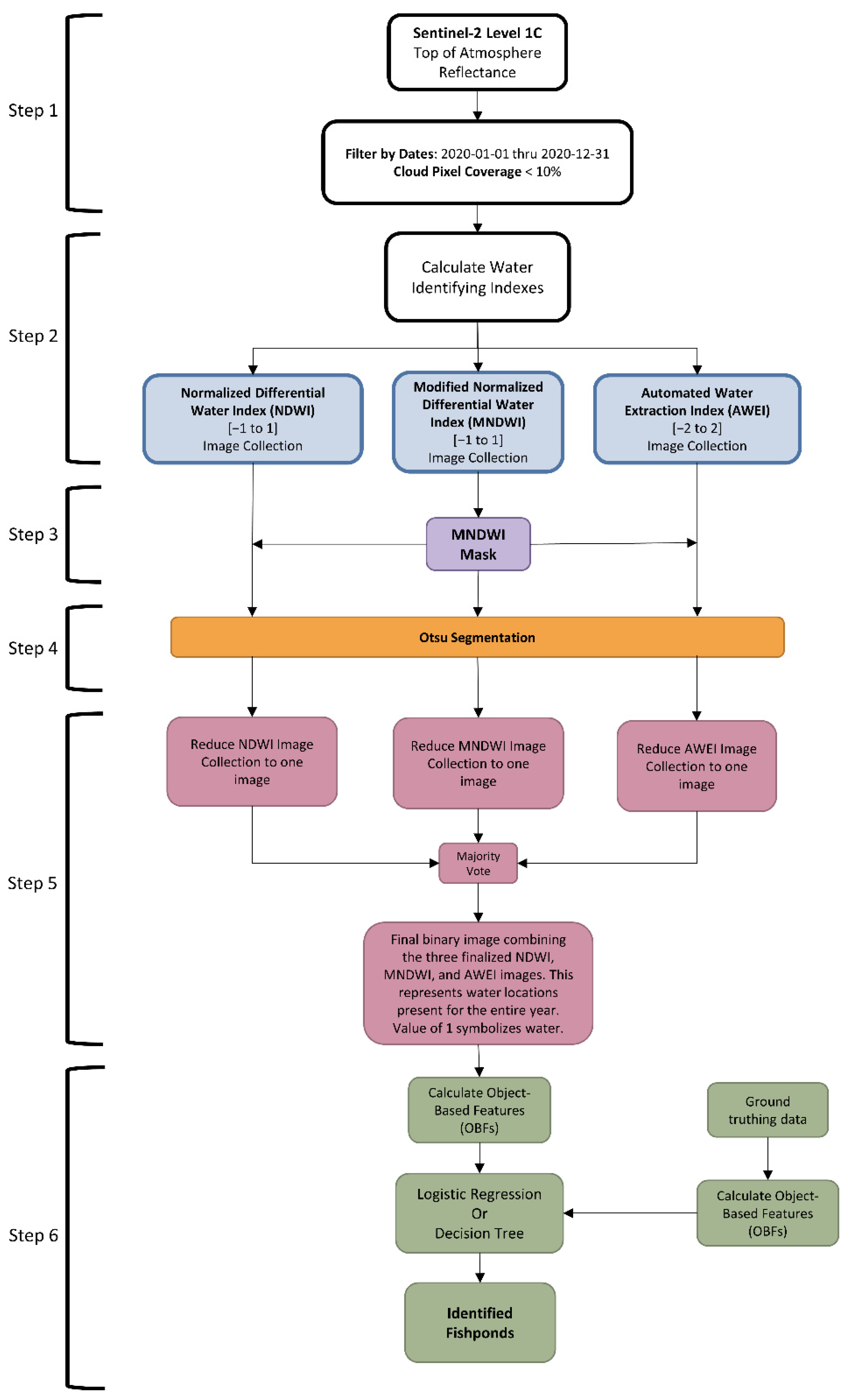
As described in the Introduction section, the Yu et al. [23] method was selected as a base method for detecting fishponds for the study area. In general, only a small number of changes (e.g., temporal and spatial extend of satellite imageries) to the original code were needed to fit the method for the study area. The base method comprises six main steps: data acquisition, water index calculation, initial mask, threshold optimization, majority vote, and fishpond identification (Figure 2).
Step 1.Data Acquisition: The process starts with combining data from Sentinel-2 Level-1C (top of atmosphere reflectance) from 1 January 2020 to 31 December 2020. Sentinel-2 collects multi-spectral data with spatial resolutions from 10 to 60 m. Sentinel-2 Level-1C bands range from visible to near-infrared and short-wave infrared. The images from these dates are then filtered for cloud coverage, keeping only those images with less than 10% cloud pixels. We obtained 311 images for our study region during 2020 that include any image that covers any part of our study region. This is one of the major differences with the original Yu et al. [23] study, as they only obtained four images for their region of interest during the study period of 2016. In addition, the size of our study region is just under 33 times larger than the Yu et al. [23] study area. During the 2020 study period, no images were available between mid-June and the end of September due to the monsoon occurrence. We identified the cloud coverage using the QA60 band available in the Sentinel-2 imagery. This band provides 60 m spatial resolution masks for opaque and cirrus clouds. Opaque clouds are determined with a thresholding technique using the blue (B2), cirrus (B10), SWIR1 (B11) and SWIR2 (B12) bands to avoid snow/cloud confusion. Cirrus clouds, which are high-altitude, thin, and semi-transparent clouds, are determined using the blue band and the B10 band corresponding to a high atmospheric absorption. In addition, morphological operations (i.e., erosion, dilation) are performed to limit false detections. We used the cloud masks to remove the corresponding pixels from the water detection analysis. In Figure S2 we present the cloud distribution for the single-day images employed in this study.
Step 2. Water Index Calculation: To identify where water is located within the study area, three different water indexes were used. These indexes analyze different wavelengths of reflected light to determine the presence of water. Using the images left after the cloud filter, we calculated the three water indexes: the normalized difference water index (NDWI) [33], the modified NDWI (MNDWI) [34], and the automated water extraction index with no shadow (AWEI) [35].
Step 3.Initial Mask: Previous studies showed that MNDWI performed the best among the three water indices [36,37,38] and also recommended by Yu et al. [23] method; the mask is created from this index. The MNDWI is filtered by the ‘greater than’ function. If an MNDWI pixel value is greater than 0, the function returns a value of 1. The filtered MNDWI images are reduced into one image using the allNonZero reducer command in the Google Earth Engine (GEE). The reducer assigns the pixel values of 0 or 1 based on all values obtained from every image in the collection at a specific location. If every value at that pixel location was a non-zero, then the final image has a pixel value of 1 at that location. If there is even one 0 value in any image at that location, then the final image has a pixel value of 0. This creates an initial binary mask that is converted to polygons. The polygons are enlarged with a buffer of 5 pixels to capture values of pixels that surround bodies of water. The polygons are then rasterized, creating a new image called MNDWI Mask (MM). The MM is then applied to the NDWI, original MNDWI, and AWEI image collections.
Step 4. Threshold Optimization: This initiates a process called Otsu segmentation which optimizes the threshold between foreground and background in images (water and not-water) [39]. The segmentation process creates a histogram of water index values from the locations the MM provided. Otsu segmentation performs best when the histogram is bimodal with a buffer of 5 pixels, the two modes being water and non-water. The threshold between the two modes is found using the sum of squares and is the optimal balance of low-intraclass variance and high inter-class variance. The Otsu segmentation process occurs within each index’s image collection separately.
Step5. Majority Vote: The optimized NDWI, MNDWI, and AWEI image collections after Otsu segmentation are then reduced into three images (one for each index) using the allNonZero reducer. This creates three separate images that show where each water index identified water in every image during the time period. The three reduced index images are then reduced to one image through the mode/majority vote method. The mode method sees what value is present at that pixel location most often and assigns the final image that value. The final combined image depicts where water is in the majority of indexes and also where water is located in every image. This image is then converted into polygons and these polygons are given object-based features (OBFs). The OBFs include the iso-perimetric quotient, solidity, patch fractal dimensions, convexity, and square pixel metric. The convexity, solidity, and path fractal dimensions describe basic geometric characteristics of the pond and how complex it may be [40]. The iso-perimetric quotient measures how similar an object is to compact shapes like circles [41]. Lastly, the square pixel metric analysis for the shape convexity and is similar to the iso-perimetric quotient [42].
Step 6. Fishpond Detection: Two machine learning techniques are utilized following the Yu et al. [23] recommendations: classification and regression trees (CART) and logistic regression (LR). These two algorithms were run in R Studio utilizing the caret package [43]. The algorithms are trained by analyzing the calculated OBFs of the ground truthing data. The base method determined algorithm performance by using five-fold cross-validation.
The base method used images from the GEE platform to determine what defined a fishpond visually. The fishponds were then manually digitized for their study area to train their algorithms. In addition, non-fishpond water bodies were identified by removing digitized lakes from the Tibetan Plateau.

2.3. Proposed Improvements

We identified Yu et al. [23] method as having the most promising and applicable methods for our region of interest in southern Bangladesh, but with some modifications. From initial surveys, we found that many of the assumptions in the Yu et al. [23] paper do not apply to the south-west and south-central regions of Bangladesh (Table 1).
In order to address these shortcomings, the following changes were proposed to improve the base method (1) to identify a period of time that all types of fishponds are filled with water, (2) to modify the buffer size to improve differentiating fishponds from their surroundings, (3) to change the image reducer and water index combination to enhance waterbody detection, (4) to introduce a convolution filter for edge detection, and (5) to utilize support vector machine (SVM) and random forest (RF) as two additional machine learning techniques, and (6) utilize ground truthing data for better algorithm training.
Improvement 1: As described earlier, the shortcoming of the base method in assuming year-round fishponds impoundment is not valid in our study region as many fishponds are dried for a certain part of the year. In addition, using many images for the entire year for a large study area, such as the one here, can significantly increase the computational time or prohibit the implementation of the base method for a large study area.
In order to address this shortcoming, we identified a period of time in which all types of fishponds are filled with water. For this period, two sets of analyses were performed. First using all images with less than 10% cloud cover over the span of one month. Secondly, in order to further reduce the computational needs for data processing in our large study region, a single image for each district during the month of interest was selected for the second set of analyses.
Using images for a single month, relevant satellite images were obtained for the period of 11 October to 13 November of 2020 instead of the full year. Therefore, the total number of images was reduced from 311 for the whole year observation to 43 for one month observation. For the second scenario, one single day during the month was selected. Since our study area is very large compared to the base method, each district has a different day that falls between 11 October and 13 November. The images chosen were based on visual inspection and clarity, such as cloud coverage and contrast between water and non-water. The days chosen for each district are shown in Table 2.
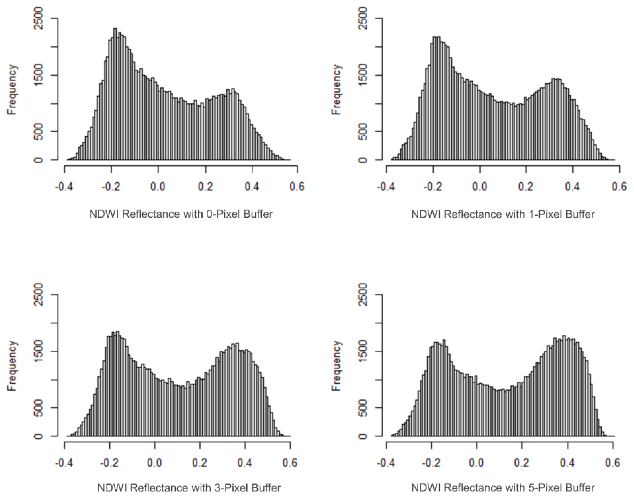
Improvement 2: The base method assumes that fishponds are surrounded by non-water pixels, but this is not the case in some of the districts in our study region. The Satkhira and Khulna districts, for example, have fishponds and agricultural fields that are very close together with dikes and buffers that are smaller than 10 m. We tested buffer sizes of 0, 1, 3, and 5 pixels to identify the best size as the buffer in the base method is a very important step in creating the MM. The MM is a binary raster that is one of the inputs into the Otsu segmentation function. Where the MM has a value of 1, the Otsu segmentation function creates a histogram of index values at those locations. The buffer selects an additional region around the areas where the MNDWI has identified water that is assumed to be land. The histogram created by Otsu should be bimodal, where one peak represents water and the other represents non-water. Having a bimodal histogram makes the threshold values from Otsu more accurate. The potential issue with a buffer of 5 pixels is that it assumes that the water bodies identified by MNDWI during the MM process are surrounded by 50 m of land, trees, or buildings. This is not the case in many of the districts in our study region. In areas where aquaculture ponds are being used, they tend to be very close together, with only a dike separating them. Dikes are much smaller than 50 m; some are even smaller than the 10 m pixel that we can see. Fishponds surrounded by other water bodies could change the histogram from bimodal to unimodal since most pixels identified by the MM are water. We wanted to see if the buffer size impacts the histogram and threshold value from the Otsu segmentation. If that threshold impacts how much water we identify and whether they have clear boundaries for a better classification.
Improvement 3: The base method functions under the assumption that water is present in fishponds throughout the year and in every image. To implement this assumption, they utilize an all-or-nothing reducer called allNonZero and combine all three water index images. We know that some fishponds are drained for maintenance or may not be visible due to an imaging error (e.g., sensor issues, platform issues, or angle issues). With the all-or-nothing style of reducer, the base method removes too many potential fishponds and under detects. Therefore, we tested an image reducer that would take the value of what is present in the majority of images instead of all.
The allNonZero reducer in the base method labels final image pixels with a value of 0 (or non-water) if even one image does not have water at that location. This is a very strict reducer that eliminates too much water during the pre-processing and establishes a lower bound estimate. It does not take into account potential cloud interference or the periods of time when ponds may be dried or have rice within them. The allNonZero reducer is used two times in the base method. The first instance is in creating the MM when combining all the MNDWI images. The second instance is when combining the calculated index images into one summary image for each index (Step 5: majority vote). The first instance of the allNonZero reducer remains the same since we want very strict water locations to create the MM. As an improvement, we replaced the second instance of the allNonZero reducer with the mode reducer. The mode reducer, instead of requiring water to be present for every image, requires that water be present for most of the images. The mode reducer allows for more water pixels to be identified in the final classification.
The base method combines images from all three water-identifying indexes together to create one final summary image. We assumed this muddles the shape and location of identified water bodies, decreasing the overall amount of detected water. To improve upon this, we tested four different index combinations to evaluate what performed best in each district. The combinations are the base method, AWEI individually, NDWI individually, and MNDWI individually. This test shows whether combining the three indexes negatively impacts the fishpond identification results or filters out likely non-fishpond water bodies.
Improvement 4: Increasing the number of water pixels, whether from reducing the time frame, changing the buffer, or using the mode reducer, causes many water bodies to merge, forming much larger polygons. This problem is exacerbated by the issue of dikes and other dividers commonly less than 10 m wide, much smaller than the best resolution images that are used in this study. These large polygons have a much higher chance of being labeled as a non-fishpond by the classifier because of their size and odd shapes. One way of breaking up the polygons is by using light detection and ranging (LiDAR) digital elevation models (DEM) to determine where raised boundaries are [45]. Unfortunately, these data do not exist in our study region. Instead, to try to reduce the size of these polygons, we introduced a Laplacian 5 × 5 convolution filter to smooth the images [46]. The convolution filter was applied to the best index or index combination image from Improvement 3 of each district and enhanced the differences between water and non-water. The convolution filter is used in ArcGIS Pro 2.4. We chose Laplacian 5 × 5 as the filter type since it visually performed better than the other filter types and has Gaussian smoothing built into the kernel (e.g., Smoothing 3 × 3, Smoothing 5 × 5, Laplacian 3 × 3).
After the convolution filter is used, we put the smoothed index image through Otsu segmentation with the MM mask. The process follows the same as the previously improved base method. This improvement aims to provide the Otsu segmentation process with a clearer index image than the one provided by the base method.
Improvement 5: The base method assumes that fishponds are easy to detect visually from standard RGB images, but that may depend more on when the images were captured and what surrounds the fishpond. Many fishponds in Bangladesh are hard to detect visually because they are surrounded by trees or many rice paddies and they have different fishpond layouts. In the study region, four types of fishponds were identified that include gher with and without rice, commercial ponds, and homestead ponds. All four types of fishponds vary in average size, typical shape, and period with water, all highlighted in Table 3. Gher without rice is, on average, much larger than all the other fishpond types. Homestead ponds and gher without rice can have round and irregular shapes, whereas gher with rice and commercial ponds typically are rectangular. The period in which each of these fishpond types is filled with water varies as well. Commercial and homestead ponds are typically permanent ponds that have water year-round. Gher can have water or not because of their design to cultivate both fish and crops throughout the year. All of these differences between fishpond types make it very difficult to locate a diverse range of fishponds visually from satellite images.
The base method utilizes historical GEE images to visually find and trace fishponds. The traced fishponds are not directly used for training, but instead, they used the shape of the polygon of water identified at the traced locations through the base method for training. For their non-fishpond data, they manually trace water bodies from a Tibetan plateau for algorithm training using the Joint Research Centre (JRC) Yearly Water Classification dataset that has a 30-m spatial resolution [47]. Tibet is north of Bangladesh and has a very different elevation and climate.
In comparison, for this study, we used 1728 ground truthing polygons provided by surveyors in Bangladesh to validate the base method’s performance and the proposed improvements. The ground truthing data consists of 996 fishponds and 741 non-fishpond waterbodies (Tables S2 and S3). Using ground truthing data additionally makes validation results reliable instead of trusting that the waterbody chosen visually was a fishpond or not. The ground truthing data was created by manually drawing borders around the known fishponds and non-fishponds in GEE. This results in the training dataset having smoother edges than what the water identification process will be. This is because the water identification process takes the shape of pixel groupings that appear blocky with hard edges. For this simplification of shape to not impact the results, we used the ‘Simplify Polygon’ function in ArcGIS to simplify the polygons identified through Steps 1–4.
Improvement 6: The two machine learning algorithms used in the base method are CART and LR due to their wide use and applications in addition of being transcribed into GEE. In addition to these algorithms, SVM [48] and RF [49] were identified as promising methods and also recommended by Maxwell et al. (2018), considering many factors such as training data, requirements, and computational cost. SVM was selected because it is useful for finding an optimal boundary between two classes [44] and performs reliably when trained with a smaller dataset [50]. RF is a larger combination of many decision trees and is easy to optimize, so it is reasonable to compare its results with the CART method [51].

2.4. Overview of the Base Method

To compare the performance of the different fishpond detection algorithms, we used several criteria, including:
(1)
The number of ground truthing fishponds that are correctly identified;
(2)
The percentage of the ground truthing area that is correctly identified by the classifier;
(3)
The number of fishponds classified;
(4)
The recall: Recall is the ratio of true positive fishponds to the total of all known fishponds, whether true positive or false negative Equation (1);
(5)
The precision: Precision is the ratio of true positive fishponds to all identified fishponds, whether true positive or false positive Equation (2);
(6)
The F1 score: The F1 score Equation (3) is the harmonic mean of the recall and precision and is used to provide a more insightful characteristic of performance than the arithmetic mean [52].
The range for recall, precision, and F1 score is 0.0 to 1.0, with 1.0 being the highest score for all of them.
R e c a l l = T P T P + F N
P r e c i s i o n = T P T P + F P
F 1   s c o r e = 2 × R e c a l l × P r e c i s i o n R e c a l l + P r e c i s i o n
To determine whether the proposed improvements significantly impacted the results, we compared the areas that are correctly identified between the base method and the proposed improvement method against the ground truthing fishpond areas. The comparison was made using a confidence interval for the mean relative error between the identified area and the known ground truthing area [53].

3. Results

3.1. Base Method Performance Evaluation within the Study Area in Detecting Waterbodies and Fishponds

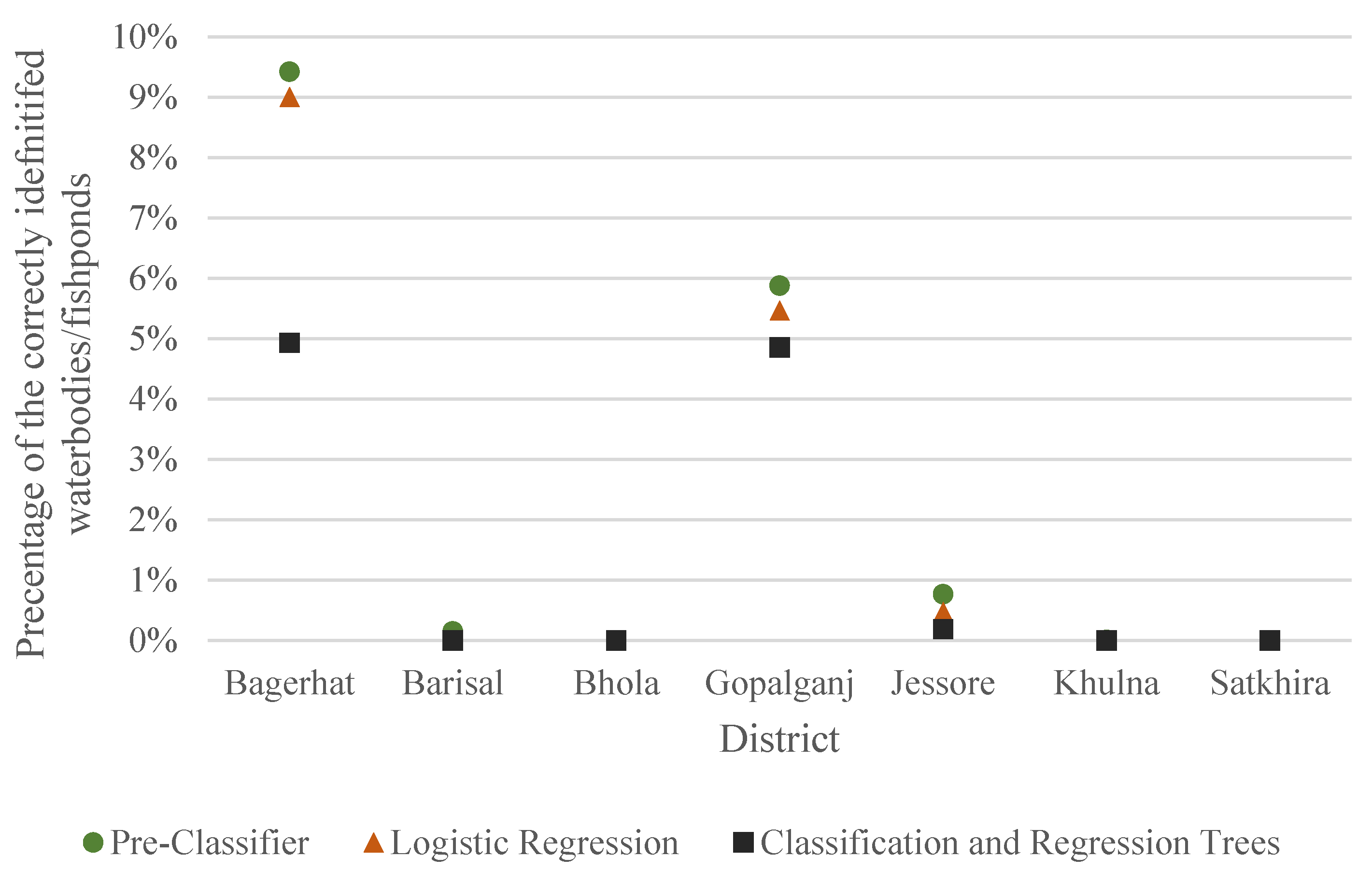
The performance of the base method was evaluated based on: (1) how well it identified water bodies and (2) how well it classified those water bodies as fishponds. Figure 3 shows the percentage of the ground truthing area that are correctly identified at pre-classifier (waterbody identification) and post-classifier (fishpond identification) stages. First, concerning detecting water areas within the known fishponds, the highest detection was in Bagerhat and had 9.4% of ground truthing fishpond area overlap. The second highest was Gopalganj with 5.9%, but the rest of the districts saw less than 1% ground truth fishpond area detection. Second, regarding the applicability of classifiers to differentiate between fishponds and non-fishponds, the LR method was identified more ground truth fishponds correctly than CART. The performance post-classifier will always be the same or less than the waterbody identification since the classifiers are only applied to the areas identified as water. Bagerhat had the highest correct classification out of the seven districts. Most of the other districts had correct classifications under 1%, except Gopalganj had around 5% classification after the LR classifier (Table S3). The CART classification true positives were lower than the LR, with the highest being Bagerhat’s 5% ground truth area identification. In Bagerhat, the base method using the LR classifier correctly identified 16 ground truthing fishponds out of 235 (9% of the total ground truthing fishpond area) (Figure 3). Having said that, still the performance of the Base Method, even in the Bagerhat, is low.
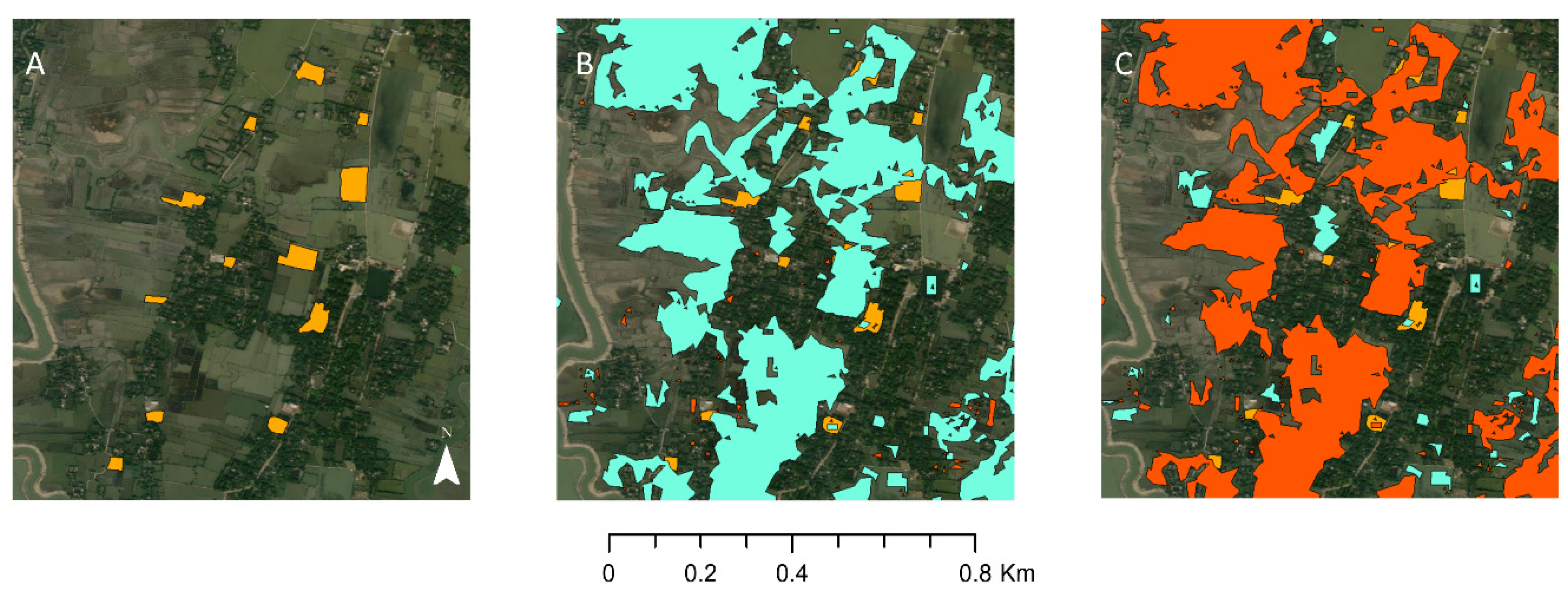
Meanwhile, the Bagerhat district is the only one of the seven in which the results are significant enough to visualize. Therefore, in Figure 4, we visually compared the performance of the classifiers that were used in the base method. While CART correctly identifies fewer ground truthing fishponds (Figure 4C), LR overclassifies water bodies as fishponds (Figure 4B). Further notable in Figure 4 are the large polygons that are identified as water and how those polygons are classified by LR and CART. LR tends to classify the large polygons as water, whereas CART is more conservative and classifies them as non-fishponds. The polygons are much larger than the ground truthing fishponds in the area, and in some cases, overlap the ground truthing fishponds. These large polygons make individual fishpond detection difficult since they typically encompass multiple fishponds or several agricultural lands (e.g., rice paddies).

3.2. Identifying the Best Period of Image Collection for Detecting Fishponds (Improvement 1)

We tested one year, one month, and one day time periods for image collection to evaluate how the number of images impacts the threshold optimization results. The one year period combined information for 311 images while one month lowered the number of images to 43. These totals are for the study area as a whole and not for each specific district. Table 4 compares the waterbody identification results from each time period. Rows 1, 3, and 5 highlight the ground truth fishpond area percentage identified and how it improves with the shorter time for every district. The district of Bhola performed the worst out of all districts with 0% water identification for both year and month periods and 3% for the day. The poor performance in Bhola could be explained by the low numbers of ground truthing data (27 locations) we have for the district. Generally, the fewer ground truthing fishponds we have, the harder it is to identify any of them specifically. Bagerhat had the best water identification during the one-month period with 52% of the ground truthing fishpond area identified, but Jessore had the best performance in a single day with 91% area identification. The districts of Barisal, Gopalganj, Khulna, and Satkhira all saw significant improvement over the base method, but performed worse than the Bagerhat and Jessore values (Tables S4–S10). All seven districts improved water identification when we changed the time period from a year to either a month or a day. The single-day images had the highest results out of the three periods. To ensure that the best time period is a day, we used both single day and single month for Improvements #2 and #3.
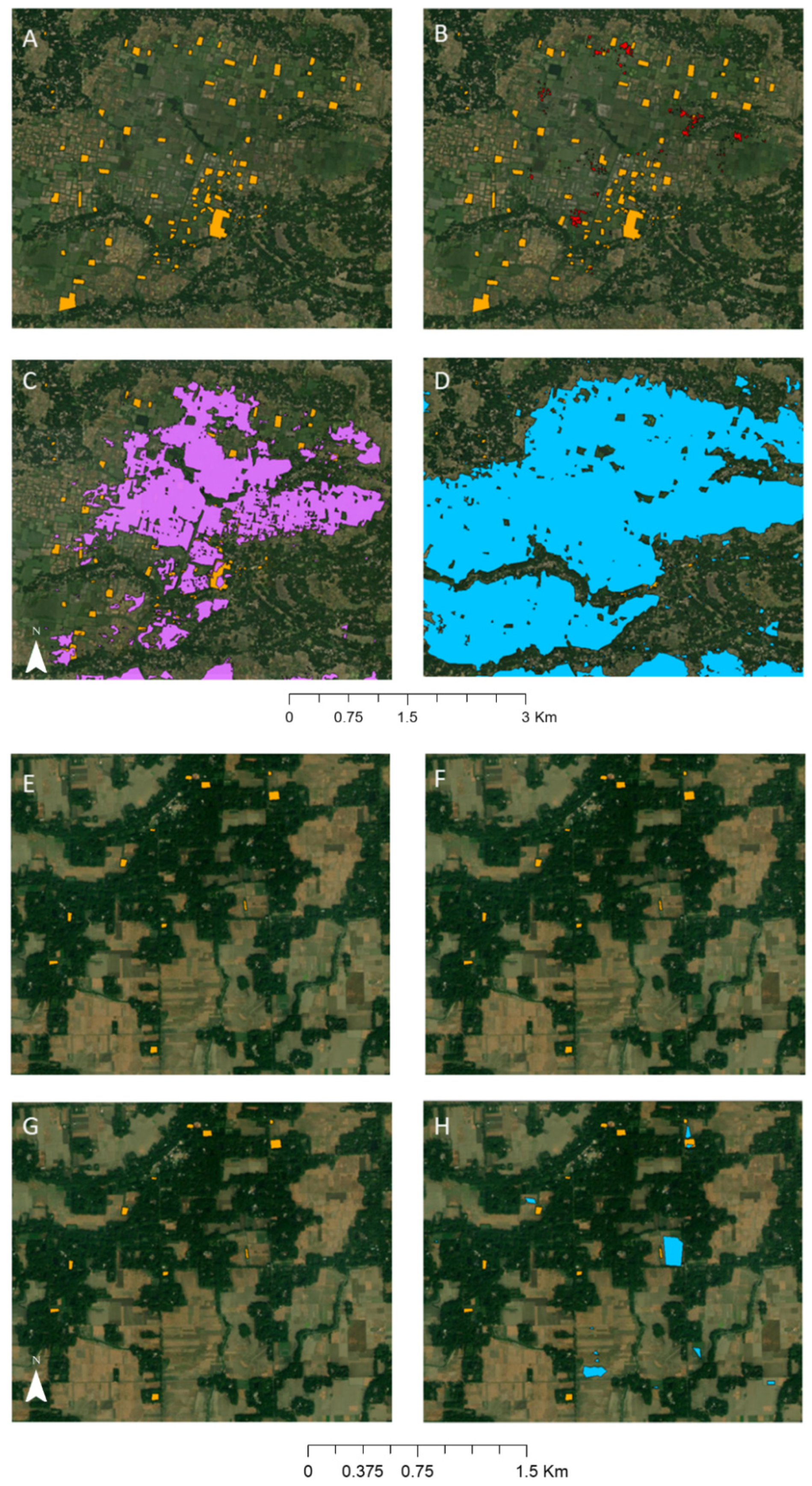
The time period of image collection proved to be a large area for improvement for identifying water. Changing the period from the full 2020 year to just 11 October to 13 November 2020 proved to be effective in identifying more water than the base method. The base method utilizes the allNonZero reducer in GEE to identify water that is present year-round. A longer time period means more images to compare and more chances for water to not be present. All districts saw an improvement in water detection from the base method and from the month period when using an image for one day. Figure 5 shows the drastic difference in water detection between the three periods, but also how small boundaries between ponds and agriculture can blend together to form large polygons. Figure 5 also compares a location in which we had good water detection, Jessore, to an area with very poor water detection, Bhola.

3.3. Testing the Buffer Size for Threshold Optimization (Improvement 2)

The buffer size impacts the amount of water identified by the Threshold Optimization process. The larger the buffer, the more pixel values are included in determining the threshold value between water and non-water. Having the best possible threshold will significantly improve upon water and fishpond identification. We tested buffer sizes of 5, 3, 1, and 0 pixels within the MM for both single day and one month time periods. The water identification pre-classifier for Bagerhat with a buffer size of 5 was 67% for one day, but that dropped to 58% with a buffer size of 0 (Table S11). This was the same trend across all districts for both time frames except for Bhola (Tables S11–S17). None of the attempted methods have resulted in any success in Bhola higher than the 3% of ground truthing area identified pre-classifier achieved from the 5-pixel buffer for a single day. The results showed that the buffer of five pixels performed better than any other size buffer for both time periods.
Figure 6 shows the histogram of NDWI values at the MM location for Khulna. The final results for each district are from using the base method, in which all three indices are combined. Khulna was chosen for the example since it had a noticeable change from the buffer size and NDWI is one of the most used water indices. The histograms for 0- and 1-pixel buffers have large peaks between −0.2 and −0.1 that represent non-water pixels. As the buffer size increases, the second peak around 0.3 to 0.4 increases considerably. With NDWI, it is commonly interpreted that values above 0.3 are water bodies and values between 0 and 0.3 may be water bodies [54]. These histograms show that with the increased buffer size, water pixels become more prominent. The 5-pixel buffer may work best because it includes more pixels in total. The more pixels included in the histogram, the more reflective the histogram is to the land use in the district. Additionally, the 5-pixel buffer works better in districts with small fishpond boundaries because it provides more opportunities for endmember pixels, or pure water pixels, to be accounted for.

3.4. Determining the Combination of Image Reducer and Water-Identifying Index to Improve Waterbody and Fishpond Detection (Improvement 3)

Both the image reducer and water-identifying indices impact the amount of water identified for classifying. The base method resulted in too few of the ground truthing fishponds being identified. Therefore, we hypothesized that determining the best combination of image reducer and indices will significantly improve the overall detections. To increase the amount of water identified, we tested two image reducers (i.e., mode and allNonZero) and four different water-identifying index combinations (i.e., AWEI, MNDWI, NDWI, and combination of AWEI; MNDWI; and NDWI). The mode reducer increased the area percentage of ground-fishponds identified for all districts (Tables S18–S24) compared to the allNonZero reducer (Tables S25–S31). The exception to this is Bhola, in which most of the results were 0% except for the NDWI index in which the Mode reducer identified 7%.
Figure 7 shows the comparison of the combined indexes, AWEI, MNDWI, and NDWI in correctly identifying the ground truth fishpond areas for each district. The combination of all three indexes that represents the base method did not perform the best for any district. Figure 7 also shows that the MNDWI by itself also does not perform the best for any district (Tables S32–S38).

3.5. Implementing Edge Detection with a Convolution Filter to Improve Fishpond Boundary Detection (Improvement 4)

Considering the results from Improvement 1 through 3, the best combination of time of image collection, buffer size for the threshold optimization, and water index for each district was identified. Two major combinations are as follows: (1) single day, 5-pixel buffer, with AWEI index for Bagerhat, Gopalganj, Jessore, and Khulna and (2) single day, 5-pixel buffer, with NDWI index for Barisal, Bhola, and Satkhira (Table S39). Since the best combination for every district entails using the single day image, the reducer type is no longer relevant. A potential reason why MNDWI does not perform to the same standards as NDWI and AWEI is that MNDWI was created to differentiate water from built-up land since built-up land can have a very similar NDWI value to water [55]. This is not necessarily an issue in our study region since there is not significant built-up land present. In fact, most of the representative fishponds (ground truth) are not located near significant developed land. Our preliminary literature review also supported this assumption that is most likely the case with the majority of fishponds in the country. In addition to this, MNDWI uses spectral bands that have 20 m spatial resolution that may decrease the accuracy of its results.
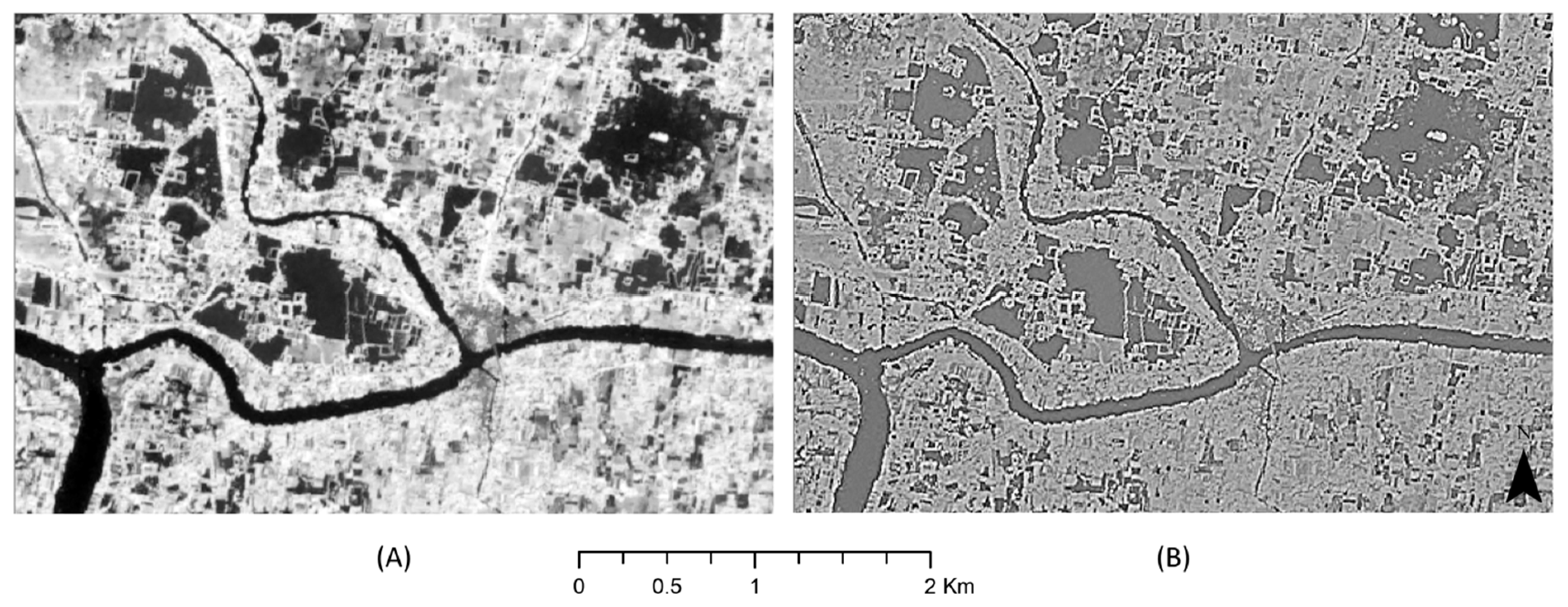
In the next step, we apply a Laplacian 5 × 5 convolution filter for edge detection to identify the best image combination for each district. The purpose of introducing edge detection is to begin with an enhanced image that highlights sharp differences in pixel values. The difference in pixel values shows where boundaries are located around different plots of land. The convolution filter emphasized the differences in the select index images to identify the boundaries around water. Figure S4 shows the results of both the Laplacian 3 × 3 and Laplacian 5 × 5 filters. The 5 × 5 filter is much more sensitive to change than the 3 × 3 filter is due to having a larger range of values than the 3 × 3. This can be seen in the legend of Figure S3. The spectrum of index values widens after the filter has been applied, allowing for differences to become more apparent numerically. For example, the original range of NDWI values in Barisal is −0.50 to 0.65. After using the filter, the range lengthens from −14.83 to 8.95. Visually, the filter highlights boundaries but does make many of the pixels become a very similar grey color (Figure 8B).
Bagerhat, Bhola, Gopalganj, Jessore, and Khulna had all their ground truthing fishponds identified before classification (Table S40). Jessore performed the best with edge detection seeing all 113 ground truthing fishponds and 91.5% of the area correctly identified before any classifier was used. Despite Jessore’s high performance, the water body identification pre-classifier decreased with adding edge-detection from 95% to 91.5%. Satkhira experienced a similar result from adding edge-detection with the ground truth area identified decreasing from 91% to 82%. Oppositely, Gopalganj, Barisal, and Bhola all increased their ground truthing fishpond area identification at the pre-classifier stage from 54% to 68%, 26% to 58%, and 20% to 57%, respectively. The same district divide was seen with the post-classifier results as well. Barisal and Bhola saw an increase in their post-classifier area identification for both LR and CART. The ground truthing fishpond area percentage for Jessore decreased from 94.3% to 91.4% with LR and from 3% to 0% with CART using edge-detection. Satkhira saw a slight increase from 0.3% to 5% for the CART classifier, but its LR dropped from 93% to 56% ground truth area identification.

3.6. Evaluating the Impact of Ground Truthing Data on Machine Learning Training (Improvement 5)

To train machine learning classifiers, the base method manually traced suspected fishponds from historical satellite images. The water bodies they traced may have only been representative of one type of fishpond because homestead ponds and gher with rice are very difficult to identify as fishponds. To improve the machine learning classifier training, we used detailed ground truthing data for all four types of ponds described previously. In addition to this, we had ground truthing data for non-fishpond water bodies that would provide juxtaposing training data.
Table 5 compares the performance of the machine learning classifiers when they are trained with ground truthing data versus historical imagery that was used in the Yu et al. [23]. The recall significantly increased from 0.538 to 0.989 for LR and from 0.495 to 0.827 for CART. This shows that the ground truthing data decrease the number of false negatives. The precision score decreased from 0.788 for LR and 0.773 for CART to 0.594 and 0.738, respectively, when using the ground truthing data for machine learning training. A decrease in precision implies an increase in the number of false positives.

3.7. Adding Random Forest and Support Vector Machine Classifiers to Determine the Best Classifier for the Data (Improvement 6)

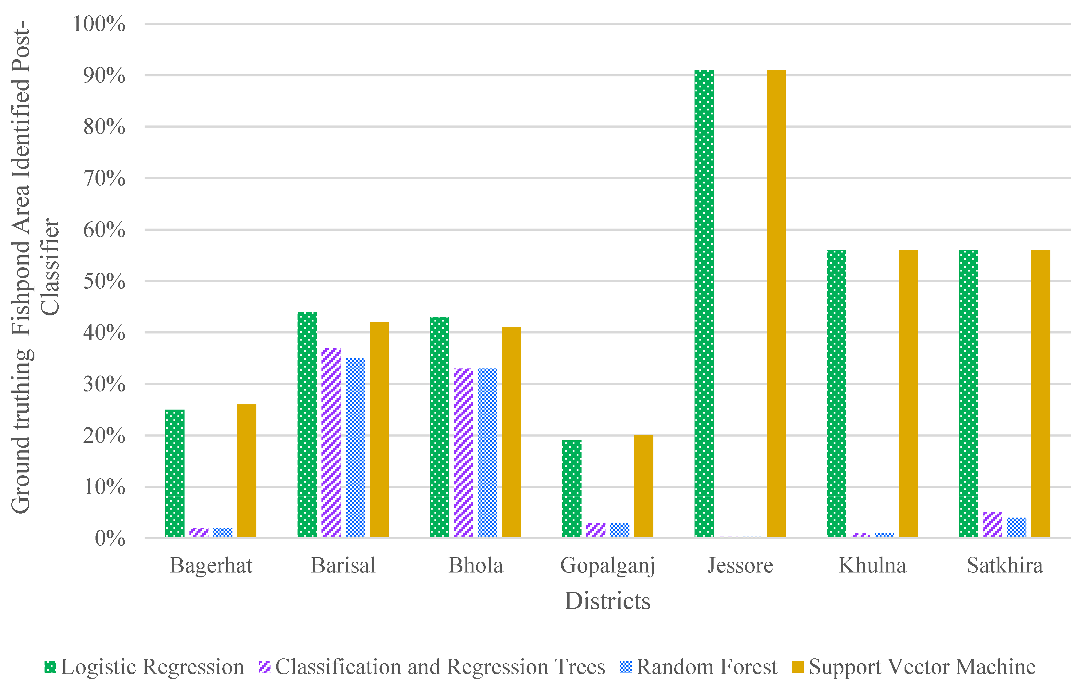
In addition to LR and CART, RF and SVM are widely recognized classifiers and can be used for many different research applications that require the differentiation of two or more classes [54,55,56]. To improve the classification results, we added RF and SVM since they are identified as promising classifiers [44]. Overall, the LR and SVM classifiers identified more ground truthing fishponds both in terms of area percentage and total number than the CART and RF (Tables S41 and S42). Figure 9 shows how the results of the RF and CART are similar to each other as well as how similar the results from LR and SVM are. The district with the best performance is Jessore, with both LR and SVM classifying 91% of the ground truthing fishpond area and all 113 ground truthing fishponds correctly. Jessore is also where there is the most drastic difference in performance by classifiers was observed. This could be due to the predominant presence of large water polygons in Jessore. LR and SVM tend to classify the large polygons are fishponds, whereas RF and CART do not. The RF and CART classifiers in Jessore performed the worst out of any district with 3% ground truthing fishpond area identification and 3 of 113 fishponds correctly identified. Introducing two additional classifier types yielded similar results to the base method. Table 6 compares the precision, recall, and F1 scores for each of the four classifier types we used.
The total number of classified fishponds for each district also supports the conclusion that CART is the best middle ground (Tables S41 and S42). Figure 10 shows the classifier results from LR, CART, RF, and SVM in Eastern Gopalganj as compared to the ground truth fishponds in that location.

3.8. Determining the Extent to Which the Improvements Works

We calculated the mean relative error for four different scenarios to determine whether the six proposed improvements considerably enhanced the capability of the base method for detecting fishponds. The scenarios that are considered here are the base method before classification, the enhanced method (considering all improvements) before classification, the base method using LR, and the enhanced method using CART. Table 7 outlines these statistics. The mean relative difference closest to 0 is the enhanced method without classifier (lower and upper limits of −34.4% and −31.3%). This means that the enhanced method is regularly 31–34% under detecting the ground truthing area. The other three scenarios had mean relative differences very close to −100%. The enhanced method CART mean relative difference was better than for the base method pre-and post-LR. This shows that the enhanced method without classification considerably improves upon the base method water identification.

3.9. High-Resolution Imagery Impacts on Results

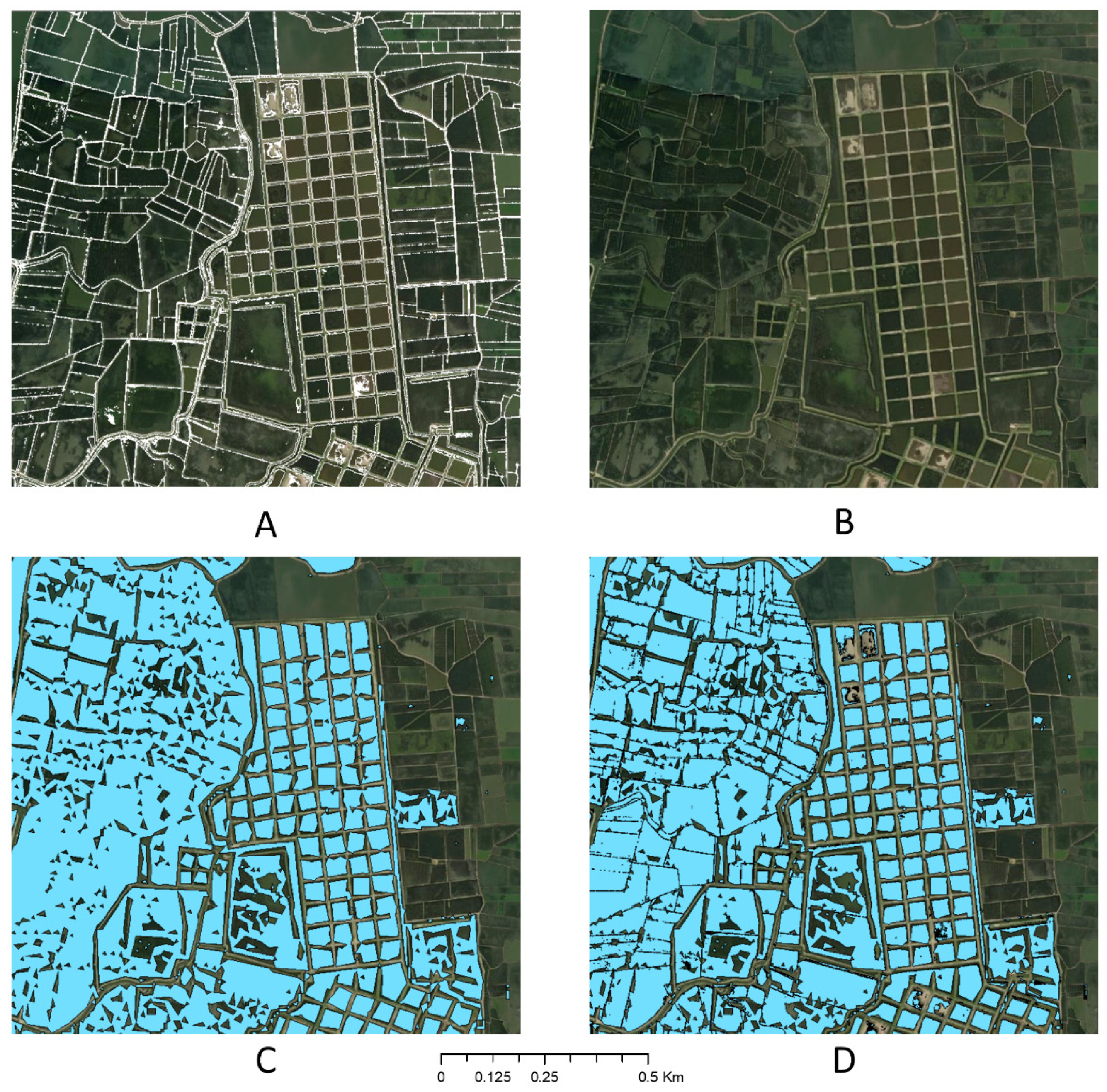
Having access to high-resolution imagery can improve the results of the enhanced method significantly. A WorldView-2 image was obtained for an area of 45 km2 in Jamalnagar, Satkhira to analyze the performance of the enhanced method. The high-resolution image was used to identify the boundaries around all land plots and intersected those boundaries with the final enhanced method for Satkhira. Figure 11 compares the boundary identification from the WorldView-2 image, the base method water identification, the enhanced method water identification, and the intersect of the WorldView-2 boundaries and the enhanced method. We applied the CART classification to the intersect of WorldView-2 and the enhanced method to compare it to the enhanced method fishpond identification alone. There are 47 ground truth fishponds in this region. The enhanced method correctly identified 9 of the 47 whereas the intersect correctly identified 29 of the 47 fishponds. In addition, the area of fishponds correctly identified was doubled with the introduction of the high-resolution boundaries. The improvement in fishpond and area identification in one small region shows that having access to high-resolution imagery would refine the results of the enhanced method even further. In summary, using high-resolution imagery would significantly improve boundary detection around fishponds and provide more accurate water locations.

4. Discussion

4.1. Implications of the Base Method

The threshold optimization (Step 4) was created to pinpoint the water bodies most likely to be fishponds. For the small study area that the base method was applied to, this technique works very well, especially since the layout of their study area has clear divided water bodies. However, even broken into the seven districts in our study area, the pixel selection technique does not perform to the same standard. The underlying assumptions of the base method are not valid for our study area and have to be adjusted to make accurate fishpond identification possible.
Overall, the base method is under-identifying water bodies before the classifier is even applied. In addition, the base method’s performance in detecting fishponds is very low, the highest of all districts being 9%, and can be enhanced significantly. In the following sections, we will evaluate the effectiveness of proposed improvements on waterbody and fishpond detections in a very large and diverse study area.

4.2. Single Day as Best Time Period

The method performs much better when using a shorter time frame with fewer images. The best period proved to be the single day. We do not expect that the day chosen will drastically impact results, but the image must have low cloud coverage (e.g., less than 10%) and it must be during a time period when we are fully confident fishponds contain water. Because of these guidelines and Bangladesh’s climate, we are only able to obtain a few images that fit these standards.

4.3. Image Reducer and Index Combination Comparisions

Testing the mode reducer on the month-long period resulted in less water identification than the single day (Tables S18–S24), but more than the same period using the allNonZero reducer (Tables S25–S31). Meanwhile, the mode reducer did improve water identification, but since single-day images only have utilized one image, the reducer has no impact on its performance.
MNDWI and AWEI performed the best out of the three indices. Using the indices alone significantly improved upon the base method combination of the three indices. Both AWEI and MNDWI were created to better differentiate water from built-up land since built-up land has similar reflectance and absorption to water. Meanwhile, the introduction of the cloud removal technique (i.e., QA60) had minimal impact (<0.21%) on the total fishponds identified.

4.4. Introducing Edge Detection with a Laplacian Convolution Filter

The results of applying the Laplacian 5 × 5 convolution filter were mixed; however, every district saw a large increase in the overall number of fishponds identified, with some now seeing over 100,000 fishponds (Table S40). The filter did succeed in dividing up large polygons of identified water, hence the large increase in overall ponds identified. The cause for why some districts saw a decrease in their overlapping area between ground truth fishponds and identified water can be attributed to the division of these polygons. The Laplacian filter identifies significant changes in neighboring pixel values, but the filter still is being used on 10 m pixels. With some 10 m pixels now being labeled as a boundary, this removes area from the water.

4.5. Creating Training Datasets from Ground Truthing Surveys and Identifying the Best Classifier for Fishpond Classification

The training datasets created from our ground truthing surveys improved both the recall and the F1 score for both LR and CART classifiers. The increases in recall and F1 score show that utilizing ground truthing data improves the performance of both the LR and CART classifiers, but the decrease in precision increases the number of false positives compared to the base method.
The F1 scores are all very similar to each other, with the range from lowest value (0.706) to highest (0.780) being only 0.074. The LR recall and precision results are interesting because it has the worst precision, but the best recall meaning the LR is very good at preventing false negatives, but the worst at preventing false positives. RF has the exact opposite results with the highest precision and the lowest recall. Both LR and RF have lower F1 scores. CART and SVM fall between LR and RF for precision and recall, but because of their consistency, they have the two higher F1 scores. From these scores, we can conclude that LR is over-classifying fishponds and RF is under-classifying fishponds. When looking at the results in Figure 10, we can conclude that since SVM performed very similarly to LR, it must also be over-classifying. In addition, since RF typically identifies less than CART and RF under-classifies, CART can be the best final option.
Since the data shows that LR is over-classifying, we can conclude SVM must also be since SVM classifies 3 to 5 times as many fishponds as LR does. This conclusion is also backed by the fact that LR and SVM are very similar classifiers, so it is realistic that they would behave similarly [57]. The CART classifier numbers always fall below LR and above RF levels. This could also support our previous finding that CART provides the best classification out of the four.

4.6. Land Use and Ground Truth Fishpond Characteristics to Explain Trends in Results

All seven districts within the study region are very different from each other. This makes creating one over-arching method very difficult. We looked at the land use surrounding the ground truth fishponds to see if there was a trend in districts that performed better/worse than others. To do this, we tested buffer sizes of 10, 50, and 100 m around ground truth fishponds in each district separately (Tables S43–S45). The predominant land use types in all districts were cultivated land, water bodies, and artificial surfaces. Bhola and Barisal had the lowest percentage of ground truthing fishpond area identified before the machine learning classifier. These two districts had the highest percentage of artificial surfaces, with Bhola seeing 73% and Barisal having just under 50% with the 100 m buffer. All other districts had artificial surfaces as 26% or less of their land use at 100 m. Water and artificial surfaces may have very similar reflectance values [58]. In this instance, since there was a very high percentage of artificial surfaces and a very low percentage of water, the indexes may be identifying artificial surfaces instead of water during Otsu segmentation.
The median size ground truthing fishpond also varied significantly by district (Table S46). The district with the smallest median size ground truthing fishpond was Bhola (713 m2), followed by Barisal (833 m2), then Satkhira (1252 m2). All other districts had median ground truthing fishponds larger than 2200 m2. The combination of having the least and smallest ground truthing fishponds may be why the improved methods performed the worst in Bhola. Barisal had more ground truth fishponds with 168, but they were additionally much smaller than other districts. This could explain why the enhanced method performed worse in Barisal than other districts.

5. Conclusions

Aquaculture is becoming increasingly important in regions that rely heavily on fish for food. Identifying where aquaculture is occurring is critical in understanding the industry, how it operates, and the areas it can improve in. With this information, we can estimate total production, inform policy, or analyze trends in aquaculture locations.
This study showed that the approach taken for identifying fishponds must be tailored to the characteristics of the fishponds, the fishponds’ surrounding areas, and the satellite data being used. The best approach for this is to test the time period for image capture, the buffer size for image optimization with Otsu Segmentation, the combination of water-identifying indexes, the image reducer type, and the machine learning classifier type. Utilizing edge-detection techniques and high-resolution imageries can improve the overall waterbody detection. For South-west and South-central Bangladesh, limiting the number of images for a specific time period results in an increased number of waterbodies detected. One reason for this is that additional errors can be introduced when combining multiple images together if an image does not capture the period with water. The buffer size for threshold optimization of water and non-water had an enormous impact on the results. The 5-pixel buffer performed the best for our study region. This proves that including more pixels in image thresholding results in better thresholds altogether, especially when the shape and size of the fishponds change throughout the year. Of the three water indices, NDWI and AWEI performed the best for the region, but this varies by location and land use/cover characteristics. The mode reducer did allow for more waterbodies to be identified than the allNonZero image reducer when working with more than one image for the study region. The image reducer type, in the end, did not matter for the enhanced method since one image is usually selected for fishpond detection. The training dataset for machine learning plays an important role in identifying the best classifier. Having diverse and representative ground truthing fishponds will improve the machine learning classifiers.
Some of the challenges that were observed in this study included (1) the size of the study area: Due to the size of the study area and the limitation of the GEE platform computational power, many of the tasks proposed in this study could not be executed for the entire region together. One way to address this issue was to divide the study area into seven districts and apply various tasks separately for each district. Meanwhile, as the computational power is increasing exponentially, it is expected that in the near future, all of these analyses can be performed within GEE without the need for dividing the study area. (2) Threshold optimization: In the original base method, one threshold value for water detection was obtained for the study region; however, our results showed that this approach does not work in a large region. Therefore, in this study, we optimized the threshold values based on the water index values at the district level. One alternative is to train the system based on the region’s physiographical and climatological characteristics instead of its political boundaries. Using the agroclimatological zone is one alternative but is not a good representation of the fishpond distribution and attributes. (3) High-resolution imagery: Our study showed that using high-resolution imagery can significantly improve the overall performance of the enhanced method in detecting fishponds. Having high-resolution imagery would be very beneficial in identifying the boundaries between fishponds and breaking up any large polygons. As the cost for high-resolution imagery decreases, these six strategies will become increasingly more useful. (4) Rainy season: The rainy and monsoon season in Bangladesh is from June through mid-October. This limits the availability of high-quality images with low cloud coverage. In fact, our study showed that the viable images for this study are mainly available from January to May and October to December. One solution can be the combined usage of SAR and optical imaging in identifying small waterbodies. Ultimately, verification of the enhanced method in other regions is crucial to examine the reliability of the proposed method. The use of a cloud mask paired with image composites through machine learning could also enhance future results by removing any cloud pixels entirely.

Supplementary Materials

The following are available online at https://www.mdpi.com/article/10.3390/rs13234890/s1, Figure S1. Land use map of the study region (adapted from (China Ministry of Natural Resources [29]); Figure S2. Distribution of ground truthing data locations by type, Table S1. Land cover as percentage of area for each district within the study region (China Ministry of Natural Resources [29]); Table S2. Numbers of ground truthing data fishponds and non-fishponds by district; Table S3. Base method comparison for all seven districts; Table S4. Time period comparison for Bagerhat; Table S5. Time period comparison for Barisal; Table S6. Time period comparison for Bhola; Table S7. Time period comparison for Gopaglanj; Table S7. Time period comparison for Gopaglanj; Table S8. Time period comparison for Jessore; Table S9. Time period comparison for Khulna; Table S10. Time period comparison for Satkhira; Table S11. Buffer size comparison for Bagerhat for both month and single day; Table S12. Buffer size comparison for Barisal for both month and single day; Table S13. Buffer size comparison for Bhola for both month and single day; Table S14. Buffer size comparison for Gopalganj for both month and single day; Table S15. Buffer size comparison for Jessore for both month and single day; Table S16. Buffer size comparison for Khulna for both month and single day; Table S17. Buffer size comparison for Satkhira for both month and single day; Table S18. Mode reducer applied for one-month period in Bagerhat comparing water-identifying index combinations; Table S19. Mode reducer applied for one-month period in Barisal comparing water-identifying index combinations; Table S20. Mode reducer applied for one-month period in Bhola comparing water-identifying index combinations; Table S21. Mode reducer applied for one-month period in Gopalganj comparing water-identifying index combinations; Table S22. Mode reducer applied for one-month period in Jessore comparing water-identifying index combinations; Table S23. Mode reducer applied for one-month period in Khulna comparing water-identifying index combinations; Table S24. Mode reducer applied for one-month period in Satkhira comparing water-identifying index combinations; Table S25. allNonZero reducer applied for one-month period in Bagerhat comparing water-identifying index combinations; Table S26. allNonZero reducer applied for one-month period in Barisal comparing water-identifying index combinations; Table S27. allNonZero reducer applied for one-month period in Bhola comparing water-identifying index combinations; Table S28. allNonZero reducer applied for one-month period in Gopalganj comparing water-identifying index combinations; Table S29. allNonZero reducer applied for one-month period in Jessore comparing water-identifying index combinations; Table S30. allNonZero reducer applied for one-month period in Khulna comparing water-identifying index combinations; Table S31. allNonZero reducer applied for one-month period in Satkhira comparing water-identifying index combinations; Table S32. Water-identifying index combination comparison for Bagerhat using single-day time period; Table S33. Water-identifying index combination comparison for Barisal using single-day time period; Table S34. Water-identifying index combination comparison for Bhola using single-day time period; Table S35. Water-identifying index combination comparison for Gopalganj using single-day time period; Table S36. Water-identifying index combination comparison for Jessore using single-day time period; Table S37. Water-identifying index combination comparison for Khulna using single-day time period; Table S38. Water-identifying index combination comparison for Satkhira using single-day time period; Table S39. Best results of the index tests for each of the seven districts; Table S40. Results from adding the Laplacian 5 × 5 convolution filter for each district; Table S41. Comparison of LR, CART, RF, and SVM results when applied to ground truthing fishpond data for Bagerhat, Barisal, Bhola, and Gopalganj during one day with that district’s best performing water-identifying index; Table S42. Comparison of LR, CART, RF, and SVM results when applied to ground truthing fishpond data for Jessore, Khulna, and Satkhira during one day with that district’s best performing water-identifying index; Table S43. Land use as percent of total area for 10 m buffer around ground truth fishpond locations for each district; Table S44. Land use as percent of total area for 50 m buffer around ground truth fishpond locations for each district; Table S45. Land use as percent of total area for 100 m buffer around ground truth fishpond locations for each district; Table S46. Median ground truth fishpond size for each district.

Author Contributions

Conceptualization, A.P.N., H.F. and J.S.H.-S.; methodology, H.F. and A.P.N.; software, H.F., J.K. and I.K.; validation, R.E. and M.M.H.; investigation, N.M. and J.S.H.-S.; data curation, H.F. and J.K.; writing—original draft preparation, H.F.; writing—review and editing, A.P.N., N.M. and B.B.; supervision, A.P.N. and N.M.; project administration, A.P.N. All authors have read and agreed to the published version of the manuscript.

Funding

The Feed the Future Innovation Lab for Fish is managed by Mississippi State University through an award from the United States Agency for International Development (USAID) (Award No. 7200AA18CA00030; M. Lawrence, PI) and provides support to this project (Grant No. 193900.312455.12B; Belton, PI; Haque, PI). This work was also supported by the USDA National Institute of Food and Agriculture, Hatch project 1019654.

Data Availability Statement

The data presented in this study are available on request from the corresponding author.

Acknowledgments

This article was made possible by the generous support of the American people provided by the Feed the Future Innovation Lab for Fish through USAID. The contents are the responsibility of the authors and do not necessarily reflect the views of USAID or the United States Government. We would like to express our appreciation for Zhiqi Yu for providing the original code for and assistance with the Base Method. We are also grateful to Jawoo Koo (IFPRI) and Aniruddha Ghosh (Alliance Bioversity-CIAT) for their help with locating high-resolution satellite images of Southwest Bangladesh.

Conflicts of Interest

The authors declare no conflict of interest.

References

  1. FAO. The State of World Fisheries and Aquaculture; FAO: Rome, Italy, 2020. [Google Scholar]
  2. Kobayashi, M.; Msangi, S.; Batka, M.; Vannuccini, S.; Dey, M.M.; Anderson, J.L. Fish to 2030: The role and opportunity for aquaculture. Aquac. Econ. Manag. 2015, 19, 282–300. [Google Scholar] [CrossRef] [Green Version]
  3. Bernzen, A.; Pritchard, B.; Braun, B.; Belton, B.; Rigg, J. Guest editorial: Geographies of engagement, livelihoods and possibility in South and Southeast Asian deltas. Singap. J. Trop. Geogr. 2021, 42, 197–202. [Google Scholar] [CrossRef]
  4. Belton, B.; Bush, S.R.; Little, D.C. Not just for the wealthy: Rethinking farmed fish consumption in the Global South. Glob. Food Sec. 2018, 16, 85–92. [Google Scholar] [CrossRef]
  5. Hernandez, R.; Belton, B.; Reardon, T.; Hu, C.; Zhang, X.; Ahmed, A. The “quiet revolution” in the aquaculture value chain in Bangladesh. Aquaculture 2018, 493, 456–468. [Google Scholar] [CrossRef]
  6. Department of Fisheries. Yearbook of Fisheries Statistics of Bangladesh 2017–18; Department of Fisheries: Dhaka, Bangladesh, 2018.
  7. Jahan, K.; Belton, B.; Ali, H.; Dhar, G.; Ara, I. Aquaculture Technologies in Bangladesh: An Assessment of Technical and Economic Performance and Producer Behavior; WorldFish: Penang, Malaysia, 2015. [Google Scholar]
  8. Belton, B.; Azad, A. The characteristics and status of pond aquaculture in Bangladesh. Aquaculture 2012, 358, 196–204. [Google Scholar] [CrossRef]
  9. Yu, Z.; Di, L.; Tang, J.; Zhang, C.; Lin, L.; Yu, E.G.; Rahman, M.S.; Gaigalas, J.; Sun, Z. Land use and land cover classification for Bangladesh 2005 on google earth engine. In Proceedings of the International Conference on Agro-Geoinformatics, Hangzhou, China, 6–9 August 2018; Institute of Electrical and Electronics Engineers Inc.: Manhattan, NY, USA, 2018. [Google Scholar]
  10. Hashem, S.; Akter, T.; Salam, M.A.; Hasan, M.T. Aquaculture planning through remote sensing image analysis and GIS tools in Northeast region, Bangladesh. Int. J. Fish. Aquat. Stud. 2014, 1, 127–136. [Google Scholar]
  11. Rhodes, C.J.; Henrys, P.; Siriwardena, G.M.; Whittingham, M.J.; Norton, L.R. The relative value of field survey and remote sensing for biodiversity assessment. Methods Ecol. Evol. 2015, 6, 772–781. [Google Scholar] [CrossRef]
  12. Anand, A.; Krishnan, P.; Kantharajan, G.; Suryavanshi, A.; Kawishwar, P.; Raj, U.; Rao, C.S.; Choudhury, S.B.; Manjulatha, C.; Babu, D.E. Assessing the water spread area available for fish culture and fish production potential in inland lentic waterbodies using remote sensing: A case study from Chhattisgarh State, India. Remote Sens. Appl. Soc. Environ. 2020, 17, 100273. [Google Scholar] [CrossRef]
  13. Ottinger, M.; Clauss, K.; Kuenzer, C. Aquaculture: Relevance, distribution, impacts and spatial assessments—A review. Ocean Coast. Manag. 2016, 119, 244–266. [Google Scholar] [CrossRef]
  14. NASA Get to Know SAR–NASA-ISRO SAR Mission (NISAR). Available online: https://nisar.jpl.nasa.gov/mission/get-to-know-sar/overview/ (accessed on 23 July 2020).
  15. Woodhouse, I.H. Introduction to Microwave Remote Sensing; Taylor & Francis Group: Abingdon, UK, 2017. [Google Scholar]
  16. Coffey, V.C. Multispectral Imaging Moves into the Mainstream. Available online: https://www.osa-opn.org/home/articles/volume_23/issue_4/features/multispectral_imaging_moves_into_the_mainstream/ (accessed on 24 July 2020).
  17. Earth Observing System Satellite Data: What Spatial Resolution is Enough for You? Available online: https://eos.com/blog/satellite-data-what-spatial-resolution-is-enough-for-you/ (accessed on 8 June 2021).
  18. Bello, O.M.; Aina, Y.A. Satellite remote sensing as a tool in disaster management and sustainable development: Towards a synergistic approach. Procedia Soc. Behav. Sci. 2014, 120, 365–373. [Google Scholar] [CrossRef] [Green Version]
  19. Zoran, L.F.V.; Ionescu Golovanov, C.; Zoran, M.A. Spectral characteristics and feature selection of satellite remote sensing data for land use/cover changes assessment in the Romanian northwestern Black Sea coastal area. In Proceedings of the Earth Resources and Environmental Remote Sensing/GIS Applications, Toulouse, France, 20–23 September 2010; Volume 7831, p. 78311P. [Google Scholar]
  20. Ottinger, M.; Clauss, K.; Kuenzer, C. Opportunities and challenges for the estimation of aquaculture production based on earth observation data. Remote Sens. 2018, 10, 1076. [Google Scholar] [CrossRef] [Green Version]
  21. Prasad, K.A.; Ottinger, M.; Wei, C.; Leinenkugel, P. Assessment of coastal aquaculture for India from Sentinel-1 SAR time series. Remote Sens. 2019, 11, 357. [Google Scholar] [CrossRef] [Green Version]
  22. Ballester-Berman, D.J.; Sanchez-Jerez, P.; Marino, A. Detection of aquaculture structures using Sentinel-1 data. In Proceedings of the European Conference on Synthetic Aperture Radar, Aachen, Germany, 5–7 June 2018; pp. 888–891. [Google Scholar]
  23. Yu, Z.; Di, L.; Rahman, M.S.; Tang, J. Fishpond mapping by spectral and spatial-based filtering on google earth engine: A case study in singra upazila of Bangladesh. Remote Sens. 2020, 12, 2692. [Google Scholar] [CrossRef]
  24. Ren, C.; Wang, Z.; Zhang, Y.; Zhang, B.; Chen, L.; Xi, Y.; Xiao, X.; Doughty, R.B.; Liu, M.; Jia, M.; et al. Rapid expansion of coastal aquaculture ponds in China from Landsat observations during 1984–2016. Int. J. Appl. Earth Obs. Geoinf. 2019, 82, 101902. [Google Scholar] [CrossRef]
  25. Stiller, D.; Ottinger, M.; Leinenkugel, P. Spatio-temporal patterns of coastal aquaculture derived from Sentinel-1 time series data and the full landsat archive. Remote Sens. 2019, 11, 1707. [Google Scholar] [CrossRef] [Green Version]
  26. Gusmawati, N.; Soulard, B.; Selmaoui-Folcher, N.; Proisy, C.; Mustafa, A.; Le Gendre, R.; Laugier, T.; Lemonnier, H. Surveying shrimp aquaculture pond activity using multitemporal VHSR satellite images-case study from the Perancak estuary, Bali, Indonesia. Mar. Pollut. Bull. 2017, 131, 49–60. [Google Scholar] [CrossRef] [PubMed] [Green Version]
  27. Feed the Future Bangladesh. Available online: https://www.feedthefuture.gov/country/bangladesh/ (accessed on 27 July 2021).
  28. China Ministry of Natural Resources GlobeLand30. Available online: http://www.globeland30.org/defaults_en.html?type=data&src=/Scripts/map/defaults/En/browse_en.html&head=browse (accessed on 30 July 2021).
  29. Momtaz, S.; Shameem, M.I.M. The Research Setting. In Experiencing Climate Change in Bangladesh; Academic Press: Cambridge, MA, USA, 2016; pp. 41–68. ISBN 9780128034040. [Google Scholar]
  30. Bangladesh Meteorological Department Maproom: Seasonal Climate Analysis. Available online: http://datalibrary.bmd.gov.bd/maproom/Climatology/Climate_Analysis/seasonal.html?resolution=0.05&YearStart=2020&YearEnd=2020&seasonStart=Jan&seasonEnd=Dec&var=Rain&yearlyStat=Mean (accessed on 30 July 2021).
  31. Bangladesh Water Development Board. Summary of Rainfall in Bangladesh for the Year 2017 & 2018; Surface Water Processing Branch: Dhaka, Bangladesh, 2019.
  32. McFeeters, S.K. The use of the Normalized Difference Water Index (NDWI) in the delineation of open water features. Int. J. Remote Sens. 1995, 17, 1425–1432. [Google Scholar] [CrossRef]
  33. Xu, H. Modification of normalised difference water index (NDWI) to enhance open water features in remotely sensed imagery. Int. J. Remote Sens. 2006, 27, 3025–3033. [Google Scholar] [CrossRef]
  34. Feyisa, G.L.; Meilby, H.; Fensholt, R.; Proud, S.R. Automated water extraction index: A new technique for surface water mapping using Landsat imagery. Remote Sens. Environ. 2014, 140, 23–35. [Google Scholar] [CrossRef]
  35. Ji, L.; Zhang, L.; Wylie, B.K. Analysis of dynamic thresholds for the normalized difference water index. Photogramm. Eng. Remote Sens. 2009, 75, 1307–1317. [Google Scholar] [CrossRef]
  36. Jiang, H.; Feng, M.; Zhu, Y.; Lu, N.; Huang, J.; Xiao, T. An automated method for extracting rivers and lakes from landsat imagery. Remote Sens. 2014, 6, 5067–5089. [Google Scholar] [CrossRef] [Green Version]
  37. Otsu, N. A Threshold selection method from gray-level histograms. IEEE Trans. Syst. Man Cybern. 1979, SMC-9, 62–66. [Google Scholar] [CrossRef] [Green Version]
  38. Jiao, L.; Liu, Y.; Li, H. Characterizing land-use classes in remote sensing imagery by shape metrics. ISPRS J. Photogramm. Remote Sens. 2012, 72, 46–55. [Google Scholar] [CrossRef]
  39. Yu, Q.; Gong, P.; Clinton, N.; Biging, G.; Kelly, M.; Schirokauer, D. Object-based detailed vegetation classification with airborne high spatial resolution remote sensing imagery. Photogramm. Eng. Remote Sens. 2006, 72, 799–811. [Google Scholar] [CrossRef] [Green Version]
  40. Frohn, R.C. The use of landscape pattern metrics in remote sensing image classification. Int. J. Remote Sens. 2007, 27, 2025–2032. [Google Scholar] [CrossRef]
  41. Kuhn, M. Building predictive models in R using the caret package. J. Stat. Softw. 2008, 28, 1–26. [Google Scholar] [CrossRef] [Green Version]
  42. Maxwell, A.E.; Warner, T.A.; Fang, F. Implementation of machine-learning classification in remote sensing: An applied review. Int. J. Remote Sens. 2018, 39, 2784–2817. [Google Scholar] [CrossRef] [Green Version]
  43. Janowski, L.; Tylmann, K.; Trzcinska, K.; Rudowski, S.; Tegowski, J. Exploration of glacial landforms by object-based image analysis and spectral parameters of digital elevation model. IEEE Trans. Geosci. Remote Sens. 2021, 1–17. [Google Scholar] [CrossRef]
  44. Gao, J.; Du, Z.; Shi, Z.; Xu, Z.; Cao, Q.; Tang, R. Switching impulse noise filter based on Laplacian convolution and pixels grouping for color images. Signal Image Video Process. 2018, 12, 1523–1529. [Google Scholar] [CrossRef]
  45. Pekel, J.-F.; Cottam, A.; Gorelick, N.; Belward, A.S. High-resolution mapping of global surface water and its long-term changes. Nature 2016, 540, 418–422. [Google Scholar] [CrossRef] [PubMed]
  46. Cortes, C.; Vapnik, V. Support-vector networks. Mach. Learn. 1995, 20, 273–297. [Google Scholar] [CrossRef]
  47. Breiman, L. Random forests. Mach. Learn. 2001, 45, 5–32. [Google Scholar] [CrossRef] [Green Version]
  48. Ramezan, C.A.; Warner, T.A.; Maxwell, A.E. Evaluation of sampling and cross-validation tuning strategies for regional-scale machine learning classification. Remote Sens. 2019, 11, 185. [Google Scholar] [CrossRef] [Green Version]
  49. Shi, D.; Yang, X. An assessment of algorithmic parameters affecting image classification accuracy by random forests. Photogramm. Eng. Remote Sens. 2016, 82, 407–417. [Google Scholar] [CrossRef]
  50. Sasaki, Y. The Truth of the F-Measure; School of Computer Science, University of Manchester: Manchester, UK, 2007. [Google Scholar]
  51. Abramowitz, M.; Stegun, C.A. Handbook of Mathematical Functions with Formulas, Graphs, and Mathematical Tables; US Government Printing Office: Dover, NY, USA, 1972; p. 14.
  52. McFeeters, S.K. Using the Normalized Difference Water Index (NDWI) within a geographic information system to detect swimming pools for mosquito abatement: A practical approach. Remote Sens. 2013, 5, 3544–3561. [Google Scholar] [CrossRef] [Green Version]
  53. Wicaksono, A.; Wicaksono, P. Geometric accuracy assessment for shoreline derived from NDWI, MNDWI, and AWEI transformation on various coastal physical typology in Jepara Regency using Landsat 8 OLI imagery in 2018. Geoplan. J. Geomat. Plan. 2019, 6, 55–72. [Google Scholar] [CrossRef]
  54. Agmalaro, M.A.; Sitanggang, I.S.; Waskito, M.L. Sentinel 1 classification for garlic L and identification using support vector machine. In Proceedings of the 9th International Conference on Information and Communication Technology, Yogyakarta, Indonesia, 3–5 August 2021; pp. 440–444. [Google Scholar]
  55. Yan, W.; Wang, R.; Shengyi, Y.; Jianping, L. Tight reservoirs classification using random forest. In Proceedings of the 3rd International Conference on Intelligent Control, Measurement and Signal Processing and intelligent Oil Field, Xi’an, China, 23–25 July 2021; pp. 1–5. [Google Scholar]
  56. Iordache, M.-D.; Mantas, V.; Baltazar, E.; Lewyckyj, N.; Souverijns, N. Application of Random forest classification to detect the pine wilt disease from high resolution spectral images. In Proceedings of the International Geoscience and Remote Sensing Symposium, Virtual, 26 September–2 October 2020; pp. 4489–4492. [Google Scholar]
  57. Zhang, J.; Jin, R.; Yang, Y.; Hauptmann, A.G. Modified logistic regression: An approximation to SVM and its applications in large-scale text categorization. In Proceedings of the Twentieth International Conference on Machine Learning, Washington, DC, USA, 21–24 August 2003. [Google Scholar]
  58. Worden, J.; de Beurs, K.M. Surface water detection in the Caucasus. Int. J. Appl. Earth Obs. Geoinf. 2020, 91, 102159. [Google Scholar] [CrossRef]
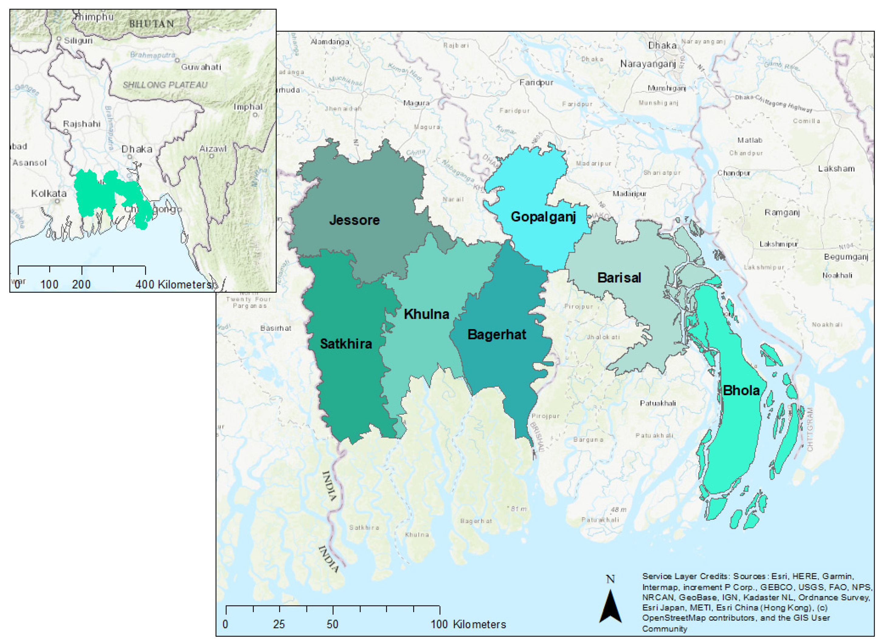
Figure 1. Study area is broken into seven individual districts.
Remotesensing 13 04890 g001
Figure 2. Flowchart outlining the major steps of the Yu et al. [23] for fishpond identification.
Remotesensing 13 04890 g002
Figure 3. Percentage of the ground truthing area that were correctly identified as waterbodies, classified as fishpond using logistic regression method, and classified using the classification and regression trees method for different districts within the study area.
Remotesensing 13 04890 g003
Figure 4. Example of the base method results in Bagerhat. Orange polygons represent ground truthing fishponds. Blue polygons are classified as fishponds. Red polygons are classified as non-fishponds. (A) Ground truthing fishponds. (B) Logistic regression classification results. (C) Classification and regression trees classification results. (Centroid of the pictures above: 22°35′59.4096″N, 89°34′57.414″E).
Remotesensing 13 04890 g004
Figure 5. Visual comparison of the three-time periods in southern Jessore and southern Bhola. (A) Jessore ground truthing fishponds (orange). (B) Jessore ground truthing fishponds and full year water (red). (C) Jessore ground truthing fishponds and one-month water (purple). (D) Jessore ground truthing fishponds and single-day water (blue). (Centroid: 22°57′49.9248″N, 89°16′46.3188″E). (E) Bhola ground truthing fishponds (orange). (F) Bhola ground truthing fishponds and full year water (red). (G) Bhola ground truthing fishponds and one-month water (purple). (H) Bhola ground truthing Fishponds and single-day water (blue). (Centroid: 22°10′7.0464″N, 90°41′27.546″E).
Remotesensing 13 04890 g005
Figure 6. NDWI reflectance values for MM in Khulna for a single-day image. Top left to bottom right: 0-pixel buffer, 1-pixel buffer, 3-pixel buffer, 5-pixel buffer.
Remotesensing 13 04890 g006
Figure 7. Ground truthing (GT) fishpond area identified pre-classifier per district for the combined index, only AWEI, only MNDWI, and only NDWI results using the single day images.
Remotesensing 13 04890 g007
Figure 8. NDWI image in western Barisal (A) before and (B) after the Laplacian 5 × 5 convolution filter was applied (Centroid: 22°51′38.37″N, 90°5′53.28″E).
Remotesensing 13 04890 g008
Figure 9. Ground truthing fishpond area percentage identified by each classifier type.
Remotesensing 13 04890 g009
Figure 10. Comparison example of classified fishponds in eastern Gopalganj using (A) logistic regression, (B) classification and regression trees, (C) random forest, and (D) support vector machine. Ground truthing fishponds are in orange and classified fishponds are in blue. (Centroid: 23°0′17.9136″N, 90°3′46.8936″E).
Remotesensing 13 04890 g010
Figure 11. Impacts of high-resolution imagery in Jamalnagar, Satkhira. (A) High-resolution boundary identification, (B) base method water identification, (C) enhanced method water identification, and (D) intersect of enhanced method and high-resolution boundaries. (Centroid: 22°34′57.6624″N, 89°12′12.1536″E).
Remotesensing 13 04890 g011
Table 1. Base method assumptions, shortcomings, and alternative approaches.
Base Method AssumptionsShortcoming of the Base Method and Alternative ApproachImprovement Number
Fishponds are filled with water year-roundSome fishpond types in Bangladesh may dry out for a portion of the year (e.g., homestead ponds). Other fishponds may be planted with rice for part of the year (e.g., Gher). Therefore, assuming all fishponds are filled with water all year is not correct. Instead of focusing on areas that have water for an entire year, we should focus on time periods when each type of fishpond holds water.1, 3
Fishponds are surrounded by non-waterBangladesh’s landscape is very diverse, and in many areas, different types of land use can be found around fishponds such as trees, rice paddies, buildings. In some regions, fishponds are very close with very narrow boundaries (<10 m apart, which is the highest resolution of imageries used here). This assumption impacts the buffer size for the MM.2, 4
Fishponds are easy to detect visually from images. Non-fishponds water bodies from another region were selected for algorithm training.There is a high probability that small fishponds cannot be detected correctly through visual observation of satellite imageries. The preferred method is to use ground truthing fishpond collections from the study region that are diverse in size, shape, type, and surrounding areas.5
CART and LR are the preferred machine learning techniques for this applicationSupport vector machine and random forest are identified as promising methods [44] for differentiating between fishponds and non-fishponds classes.6
Table 2. Date chosen for single image analysis for each district of the study region.
DistrictDate Chosen for Single Image Analysis
Bagerhat28 October 2020
Barisal13 October 2020
Bhola7 November 2020
Gopalganj28 October 2020
Jessore5 November 2020
Khulna7 November 2020
Satkhira5 November 2020
Table 3. Average size, shape, and period with water for gher with and without rice, commercial ponds, and homestead ponds.
CharacteristicGher with RiceGher without RiceCommercial PondHomestead Pond
Average size (m2)1620–202040471620810
Typical shapeRectangularRectangular, but could have curved edgesRectangularRound
Period with waterMay–DecemberFebruary–DecemberYear-roundYear-round
Predominant farming systemFreshwater prawn, fish, rice, and vegetablesShrimp and fishFishFish
Table 4. The percentage of ground truthing fishponds area and total ground truthing fishponds correctly identified in all districts using different lengths for image processing (i.e., the entire year, one month, one day).
Period of Image CollectionPerformance CriteriaDistrict
BagerhatBarisalBholaGopalganjJessoreKhulnaSatkhira
One yearPercentage of GT * fishpond area identified pre-classifier9.4%0.2%0%6%1%0.01%0%
GT * fishponds identified25 of 2351 of 1680 of 277 of 7713 of 1131 of 1630 of 208
One monthPercentage of GT * fishpond area identified pre-classifier52%4.3%0%22%44%36%66%
GT * fishponds identified139 of 2358 of 1680 of 2744 of 7770 of 11371 of 16375 of 208
One dayPercentage of GT * fishpond area identified pre-classifier67%16.3%3%36%91%67%85%
GT * fishponds identified182 of 23528 of 1681 of 2766 of 7799 of 113112 of 163115 of 208
* Ground truthing.
Table 5. Comparing statistics from Yu et al. [23] machine learning training with historical imagery to our ground truthing data training.
Training MethodPerformance CriteriaLogistic RegressionClassification and Regression Trees
Yu et al. [23]
Historical imagery
Precision0.7880.773
Recall0.5380.495
F1 Score0.6400.604
Ground truthing data Precision0.5940.738
Recall0.8980.827
F1 Score0.7150.780
Table 6. Comparing the training performance of the four classifiers on the validation ground truthing data.
Performance CriteriaLogistic RegressionClassification and Regression TreesRandom ForestSupport Vector Machine
Precision0.5940.7380.7840.720
Recall0.8980.8270.6450.822
F1 Score0.7150.7800.7060.768
Table 7. The lower and upper limits for the mean relative difference of the based and enhanced methods performances before and after a machine learning classifier.
ScenariosMean Relative Difference
Lower LimitUpper Limit
Base method before classifier−99.4%−98.5%
Enhanced method before classifier −34.4%−31.3%
Base method with logistic regression−99.7%−97.7%
Enhanced method with Classification and regression trees−91.5%−88.6%
Publisher’s Note: MDPI stays neutral with regard to jurisdictional claims in published maps and institutional affiliations.