A Spatial-Spectral Feature Descriptor for Hyperspectral Image Matching

Abstract

Hyperspectral Images (HSIs) have been utilized in many fields which contain spatial and spectral features of objects simultaneously. Hyperspectral image matching is a fundamental and critical problem in a wide range of HSI applications. Feature descriptors for grayscale image matching are well studied, but few descriptors are elaborately designed for HSI matching. HSI descriptors, which should have made good use of the spectral feature, are essential in HSI matching tasks. Therefore, this paper presents a descriptor for HSI matching, called HOSG-SIFT, which ensembles spectral features with spatial features of objects. First, we obtain the grayscale image by dimensional reduction from HSI and apply it to extract keypoints and descriptors of spatial features. Second, the descriptors of spectral features are designed based on the histogram of the spectral gradient (HOSG), which effectively preserves the physical significance of the spectral profile. Third, we concatenate the spatial descriptors and spectral descriptors with the same weights into a new descriptor and apply it for HSI matching. Experimental results demonstrate that the proposed HOSG-SIFT performs superior against traditional feature descriptors.

1. Introduction

Hyperspectral remote sensing application has made significant progress in the past few years [1] and shown competitive performance in a wide range of fields from remote sensing to biomedicine [2,3,4,5,6,7,8]. Hyperspectral image (HSI) matching is essential for hyperspectral applications but lacking attention. Therefore, constructing an HSI descriptor with good discriminative power and matching performance is of significant importance to a large number of hyperspectral vision tasks [9,10]. On the contray, feature matching algorithms are prosperous for grayscale images and applied in many vision tasks, e.g., image mosaic [11,12,13], image registration and fusion [14,15], structure-from-motion [16,17,18] and image-based localization [19,20].

Different from the grayscale image, HSI is represented as a three-dimensional ($x,y,\lambda$) data cube, where x and y represent two spatial dimensions of the scene, and $\lambda$ represents the spectral dimension (comprising a range of wavelengths) [21,22]. In other words, HSI contains a sequence of scalar image which represents a narrow wavelength range of the spectrum [23], providing much spectral information. Such spectral information includes distinct material properties of objects, offering the potential to improve the overall performance of the initial matching. Although spatial descriptors are spatially structural distinct, invariant to rotation and some certain geometric transformations with the advantage of difference of Gaussian (DOG) function and histogram of gradient (HOG), they are not designed for HSI matching. When applied in HSI, the spatial descriptors usually extract features on a single band or on a grayscale image produced by reducing the dimension of the HSI. In this way, the spectral information is ignored, which is significant to distinguish objects with similar appearances but different materials. Therefore, spatial descriptors do not perform well in the HSI matching task since they are not designed for it and do not exploit the superiority of HSI.

On the other hand, methods are applied for HSI matching by extending the 2D feature extraction function into 3D space, such as 3D SIFT [24], 3D gray level co-occurrence matrix [25] and 3D wavelet transform [26]. To use spectral information, developing descriptors which describe data distribution in both spatial and spectral domains is a natural solution [27]. Spatial and spectral scale descriptors are constructed depending on the corresponding 3D voxels. These methods can serve as the basic tools for HSI processing tasks. However, simply extending the 2D feature extraction function into 3D space ignores the physical significance of HSI that the spectral profile in each pixel represents the unique components of objects. Meanwhile, existed spectral descriptor such as SS-SIFT [28] takes advantage of spatial and spectral features by 3D HOG that breaks the continuity of spectral profile and the whole process is time-consuming. Although these methods can extract spectral and spatial features of multiband image, the performance for HSI matching is still limited in accuracy and efficiency.

Generally, feature descriptors elaborately designed for HSI matching are still in short. We consider that existing descriptors perform limitedly for HSI matching from two aspects. (1) The spatial descriptors extract features on a single band by reducing the dimension of the HSI that ignores the spectral information. Therefore, these descriptors are failed to distinguish objects with similar appearance but different materials. (2) The existing spectral descriptors ignore the physical significance that breaks the continuity of spectral profile and makes the whole process time-consuming.

Regarding the aforementioned issues, we propose a descriptor named HOSG-SIFT for HSI matching, which applies the HOSG (Histogram of Spectral Gradient) to represent the spectral features. For the first problem, HOSG-SIFT extracts the spatial and spectral features simultaneously to construct a feature descriptor. In this way, our descriptor can recognize objects with different materials but similar appearances. For the second problem, we apply HOSG to define the spectral descriptors that preserve the physical significance of the spectral profile. Moreover, HOSG can effectively reduce the reversed impact caused by unstable imaging conditions.

In summary, the main contributions of this work lie in the following two folds. First, this paper presents a spatial-spectral descriptor for HSI matching, considering the spatial and spectral information simultaneously. The proposed method performs superiority compared with state-of-the-art spectral descriptors. Second, HOSG is first used to construct the spectral descriptor, which effectively preserve the physical significance of the spectral profile.

The remainder of this paper is organized as follows. Related works on spatial feature extraction and spectral feature extraction methods are discussed in Section 2. The proposed HOSG-SIFT and its key steps, including dimensionality reduction, spatial interest points detection and local spectral descriptors construction, are described in Section 3, which effectively promotes the spectral feature extraction tasks. Experiments are introduced and analyzed in Section 4. Section 5 and Section 6 present the discussion and conclusion, respectively.

2. Related Work

2.1. Spatial Descriptors

Feature descriptors for grayscale image matching are pretty mature in many vision tasks [29]. Among them, SIFT [30] has been one of the most successful algorithms for more than a decade. Inspired by SIFT, methods including SURF [31], ROOT-SIFT [32], PCA-SIFT [33] and DSP-SIFT [34], have been proposed to promote the performance of descriptors. Specifically, SURF accelerates SIFT by approximating the Hessian matrix-based measure for the detector and a distribution-based descriptor. PCA-SIFT applies the Principal Component Analysis (PCA) algorithm to normalized gradient patch-based SIFT interest points. DSP-SIFT modify the SIFT descriptors by domain-size pooling. Additionally, in recent years, learning descriptors are proposed for grayscale image matching, performing better than the hand-craft descriptors in terms of discriminative ability [35,36,37,38].

However, the fore-mentioned spatial descriptors are elaborately designed for grayscale or RGB image with notable performance. When applied to HSI matching, spatial features are usually extracted on a single band without using the superiority of spectral information which is beneficial to improve the performance of feature descriptors.

2.2. Multidimensional Descriptors

Multimodal image, which can be regarded as an n-dimensional (N-D) data cube, is structurally similar to the hyperspectral image in some aspects [39]. Multidimensional descriptors, designing for multimodal image matching and performing well in specific applications, can be used for HSI matching directly. Methods developed from SIFT utilize the multidimensional information to present multimodal image features. Particularly, n-dimensional scale invariant feature transform (N-SIFT) [40] uses hyperspherical coordinates for gradients and multidimensional histograms to create the feature vector from multimodal medical image. 3D-SIFT [41] is proposed for action recognition based on extracting repeatable keypoint features from video data. This work shows the feasibility of 3D SIFT used for spatial-temporal data. In addition, the work [42] presents a method for volumetric image registration by making changes to orientation assignment and gradient histograms based on 3D SIFT.

Although HSI is similar to multidimensional image and can be regarded as an N-D data cube, HSI has different physical significance from other types of N-D data. The spectral dimension feature of HSI corresponds to continuous reflectance change across wavelengths, while the counterpart indexes time or spatial location in videos or medical image. In other words, each spectral dimension of HSI has similar spatial construction, while the spatial features of videos and medical image change a lot in each slice. Such differences between HSI and other N-D images should be considered when developing 3D SIFT for HSI to construct the spectral descriptors.

2.3. Hyperspectral Descriptors

Few efforts are made to explore the HSI matching. Dorado-Muñoz [43] proposed a vector SIFT detector for HSI, improving the edge performance by taking the vectorial nature of the HSI into account. The multiscale representation of the HSI is generated by vector nonline diffusion. Additionally, spectral-spatial scale invariant feature transform (SS-SIFT) [28] is designed for HSI matching. It adopts the 3D Gaussian filter and 3D-DOG to detect keypoints in spectral and spatial domains simultaneously. After that, two descriptors are proposed for each keypoint by exploring the distribution of spectral-spatial gradient magnitude in its local 3D neighborhood. However, using 3D-DOG breaks the continuity of spectral signature, which reflects the features of objects.

In general, more works should be made to promote HSI matching. The performances of spatial descriptors are limited since they are designed for grayscale image without using spectral information. On the other hand, for multidimensional descriptors, the differences in physical significance between HSI and other N-D images are failed to be considered. Moreover, the existing HSI descriptors break the continuity reflectance of the spectral profile, depressing the effectiveness of methods.

3. Method

HSI augments the spectral information of grayscale or RGB image, yet spectral information is usually ignored by state-of-the-art spatial descriptors. Meanwhile, existing spectral descriptors break the continuity of spectral profile. Spectral gradient [44] provides a material descriptor invariant to geometry and incident illumination with high performance. Thus, this paper proposes a method to construct HSI descriptors based on HOSG.

In this section, we introduce the overall framework of HOSG-SIFT construction. To clarify our approach straightforwardly, we apply Unmanned Aerial Vehicle (UAV) HSIs to display keys steps in this section. More details of UAV HSIs are illustrated in Section 4.1. Figure 1 depicts the overall structure of the proposed method. The main steps are as follows:

(1)

Spatial descriptors construction. There are two steps to construct spatial descriptors. The first step is to extract spatial interest points from an HSI in a new space produced by dimensional reduction. The second involves descriptors generating which describes the image spatial feature.

(2)

Spectral descriptors construction. After obtained the spatial interest points, we construct the spectral descriptors from the spectral gradient of surrounding neighbors. HOSG is used to construct the spectral descriptors. Additionally, normalized methods are used to eliminate the influences caused by incident changes in the environment.

(3)

A combination of the spatial and spectral feature. We obtain a spatial-spectral descriptor of 256 elements by concatenating the spatial descriptor of 128 elements and the spectral descriptor of 128 elements. The spatial and spectral descriptors have the same weight.

3.1. Spatial Descriptor

3.1.1. Dimensional Reduction by PCA

HSI contains much information and generates better discriminant performance for many applications. However, for a number of narrow bands, they have a strong correlation that results in massive redundant information in HSI. The strong correlation between several narrow bands results in massive redundancy in HSI such that it is more challenging to process HSI. Additionally, the redundancy in HSI may have a negative impact on spectral feature extraction. To resolve this problem, we transform the original features into a new space by PCA algorithm. Then, the feature keypoints and descriptors are generated in the new space.

PCA [45] is the process of computing the principal components and using them to perform a change of basis on the data, always using only the first few principal components and ignoring the rest. In fact, the PCA projects along the eigenvectors of the covariance matrix corresponding to the largest eigenvalues, where the eigenvectors points in the direction with the highest amount of data variation. Figure 2 shows the results of applying PCA with the UAV HSIs dataset.

From Figure 2 and

Table 1. The number of detected points using sift of each image.

Source Image	Figure 2a	Figure 2b	Figure 2c	Figure 2d
number of detected points	582	728	345	5455

, it can be observed that using the first principal component of HSI produces more spatial interest points than single band image. More detected keypoints allows higher number of matches and inliers (correct matched). The number of matches and inliers has a great impact on following applications, such as image mosaic, 3D-reconstruction.

3.1.2. Spatial Descriptor Construction

Grayscale images have been obtained by reducing the dimension of HSI in the last section. The next step is to construct the local spatial feature based on grayscale image. Local spatial features typically involve three distinct steps: keypoint detection, orientation estimation and spatial descriptor extraction. SIFT is used to extract spatial features in this work. The main steps of SIFT algorithm are as follows:

(1)

Local extremum detection. Local extremum points are identified by constructing a Gaussian pyramid and searching for local peaks in a series of DOG images. Taylor expansion is also applied to get the interpolated estimate for a more accurate local extremum. Moreover, candidate interest points are eliminated if found to be unstable.

(2)

Dominant orientation assignment. To achieve invariance to image rotation, dominant orientation are assigned to each keypoint based on local image properties. An orientation histogram is formed from the gradient orientation of sample points within a region around the keypoint.

(3)

Keypoint descriptors. A keypoint descriptor that should be highly distinctive and invariable to some environmental variations is then created by first computing the gradient magnitude and orientation at each image sample point in a region around the keypoint location. Figure 3 illustrates an example of constructing a spatial descriptor.

3.2. Spectral Descriptor

Taking advantage of the spectral structure to build feature descriptors is beneficial to HSI matching. Generally, 3D HOG is used to construct the spectral descriptors, yet it is time-consuming. In addition, 3D HOG ignores the physical significance of HSI that the spectral profile in each pixel represents the unique components of objects.

The appropriate description for the spectral feature is a benefit to distinguish different objects with similar appearance but different spectral features. Spectral gradient, which is commonly used in many HSI applications, describes the spectral profile rather than the original one with the advantage of reducing the magnitude offsets caused by illumination change and other impact factors. The difference between the original spectral profile and spectral gradient profile is shown in Figure 4. Meanwhile, Using spectral gradient avoids the destruction of spectral profile and save the computing time of spectral features.

Different from 3D HOG, we build the spectral descriptors using the HOSG. As shown in Figure 5, the main steps to generate the spectral descriptors are as follows:

(1)

Keypoints assignment. Same as SIFT, the potential keypoints, which should be invariant to scale and orientation, are identified by using a DOG function. Thereby, the coordinate and orientation of each spatial keypoint are determined and applied to construct the spectral descriptors

(2)

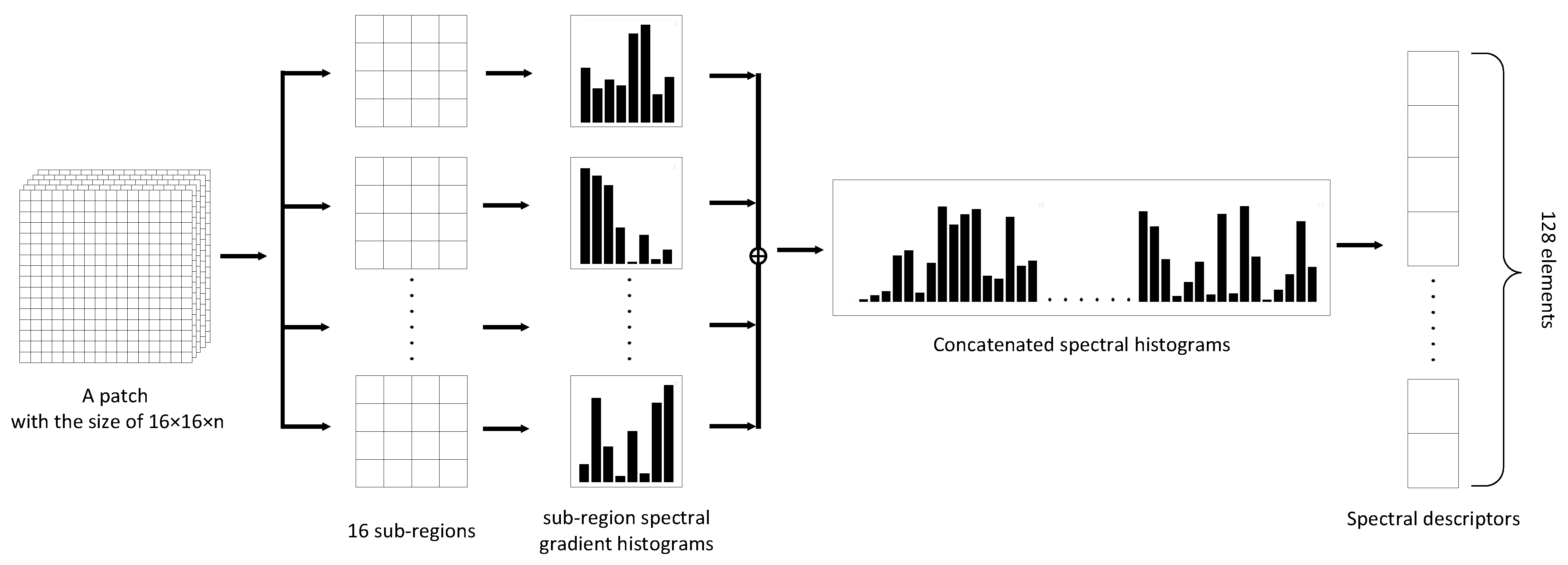
Sub-region division. We first designate a $16\times 16\times n$ (n is the number of spectral bands) patch surrounding the centre of each keypoint and rotate it to align its orientation assigned by previous step. Then, the patch is split up regularly into 16 sub-regions with a size of $4\times 4\times n$.

(3)

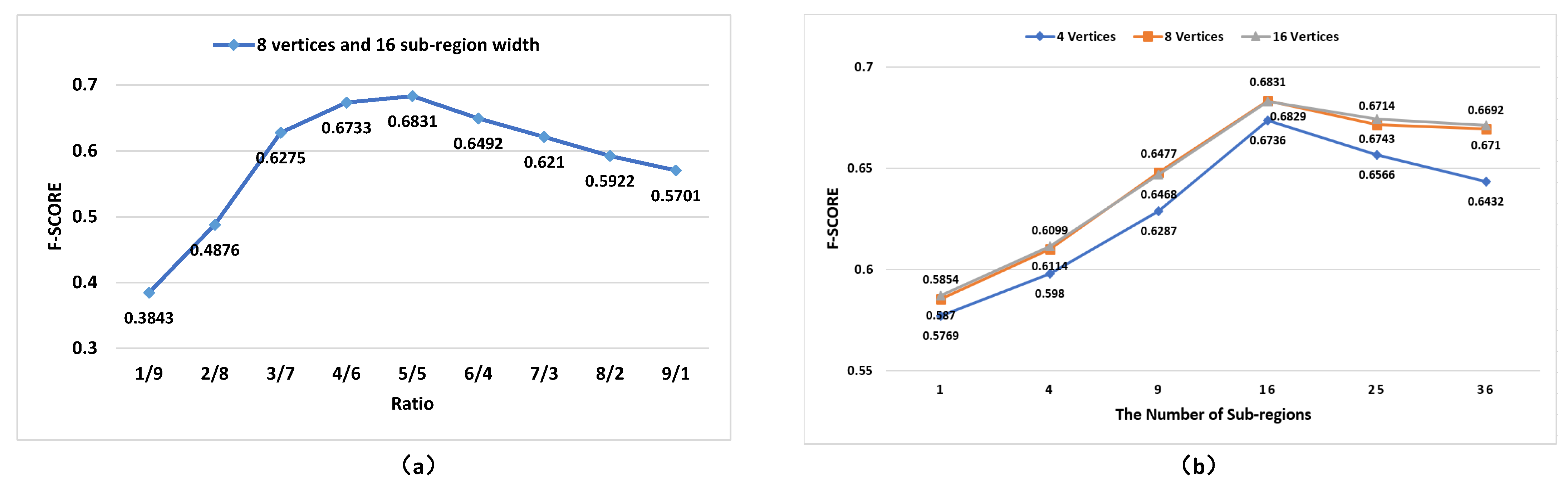
Vertices division. In this paper, the spectral gradient is evenly divided into eight vertices whose magnitude primarily ranges from −0.04 to 0.04. However, a few spectral gradient values are larger than 0.04 or smaller than −0.04. According to our statistics, most of those values are abnormal caused by the unstable imaging state of the hyperspectral sensor. Thus, we modify them to moderate the adverse effects. Specifically, the values smaller than −0.04 are increased to −0.04, while the values larger than 0.04 are decreased to 0.04. Moreover, most datasets of HSI have a similar range of spectral gradient magnitude (−0.04 to 0.04) after normalization. In this case, we believe the range (−0.04 to 0.04) can be applied to most HSI datasets.

(4)

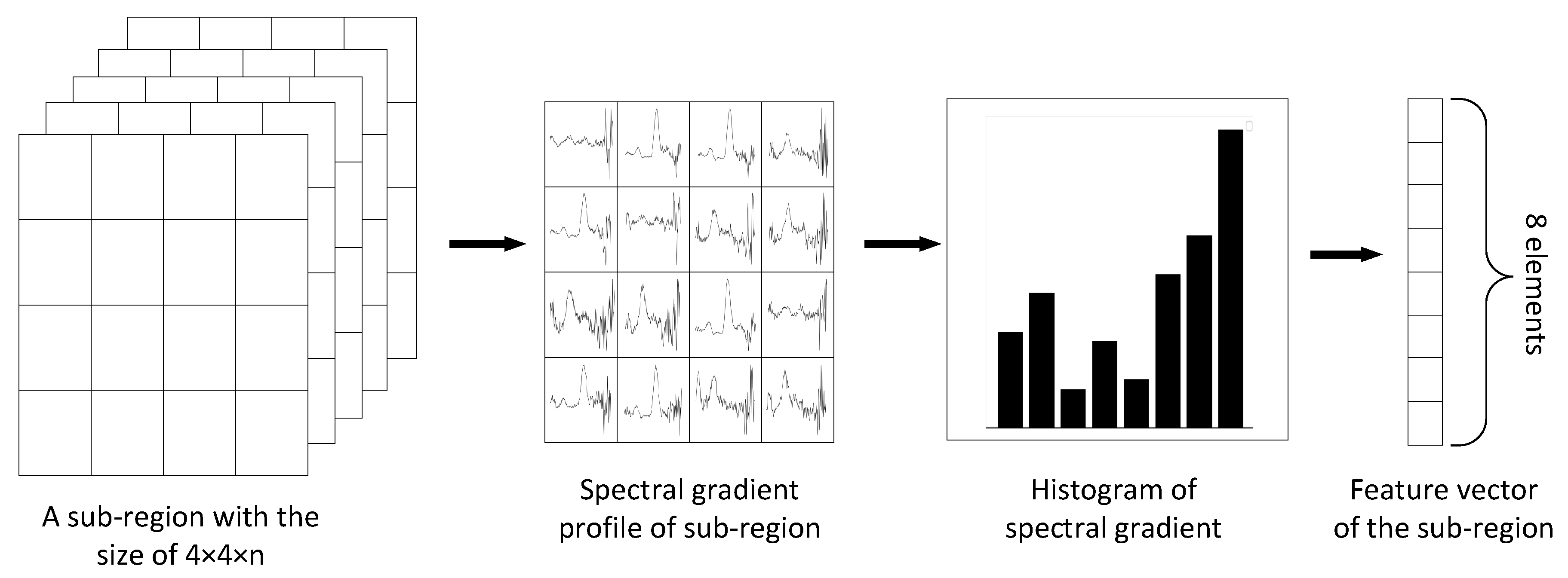
Extracting the HOSG of the sub-region. The main steps of extracting the HOSG of a sub-region is depicted in Figure 6. Specifically, the spectral gradient profile is first calculated for each pixel in the sub-region. Second, we obtain a gradient histogram for the sub-region by accumulating the spectral gradient magnitude into eight vertices, which summarizes the contents of the sub-region. Finally, a vector with eight elements is constructed to represent HOSG of a sub-region.

(5)

Spectral feature vector construction and normalization. Based on the previous steps, we obtain 16 vectors from one patch, which respectively represent 16 sub-regions. Consequently, a spectral feature vector of $8\times 16$ elements is constructed for each keypoint by concatenating the vectors of sub-regions. In that way, our method preserves the physical significance of HSI. In addition, the spectral descriptor should be normalized to reduce the negative impacts resulting from the changes in incident illumination. Specifically, the spectral feature vector is firstly normalized to the range of [−1,1]. A change in spectral profile in which each pixel value is multiplied by a constant will multiply gradients by the same constant, so this change will be canceled by vector normalization. Therefore, the descriptor is invariant to spectral changes. After that, we update the large gradient magnitudes by thresholding the values in the feature vector to each be no larger than 0.2 and no smaller than −0.2, and then renormalizing to the range of [−1,1]. This means that matching the magnitudes for large gradients is no longer as important, and that the distribution of orientations has greater emphasis. Note that the threshold values of 0.2 and −0.2 are commonly used for feature vector normalization in many works, such as SIFT [30], 3D-SIFT [24], and SS-SIFT [28], to reduce the negative impacts resulting from the changes in incident illumination.

3.3. Spatial-Spectral Descriptor

We obtain a spatial descriptor of 128 elements by SIFT and a spectral descriptor of 128 elements by HOSG, of which the method are detailedly depicted in Section 3.1 and Section 3.2, respectively. In this section, we introduce the construction of spatial-spectral descriptor, which is effective for HSI matching.

Spatial-Spectral Descriptor Construction

Based on the previous steps, we construct the spatial-spectral descriptor of 256 elements by concatenating the spatial and spectral descriptors. Considering that the weights of two feature vectors may influence the performance of the spatial-spectral descriptor, a comparison test of descriptors weights is conducted. Specifically, we assume that the weights of the spatial and spectral descriptors are w${}_1$ and w${}_2$, respectively. The sum of w${}_1$ and w${}_2$ is one (i.e., $w_1+w_2=1$). And the ratio of w${}_1$ and w${}_2$ is set to $1/9$, $2/8$, $3/7$, $4/6$, $5/5$, $6/4$, $7/3$, $8/2$, and $9/1$ for comparison test. The performance of the spatial-spectral descriptor with different w${}_1$ and w${}_2$ is shown in Figure 7a.

As shown in Figure 7a, the spatial-spectral descriptor performs the best with the weight ratio of $5/5$. It tells the spatial and spectral descriptor are equally important for HSI feature representation. Consequently, in our method, we concatenate two vectors (the spatial and the spectral descriptor) of 128 elements with the same weights to obtain the spatial-spectral descriptor of 256 elements.

3.4. Evaluation Metrics

In our experiments, some popular metrics are used to evaluate the performance of HOSG-SIFT on a per-image pair basis, including recall, precision, putative match ratio, matching score and F1-score.

Recall measures the ability of descriptor to identify the possible correct matches.

$$\mathrm{Recall}=\frac{\mathrm{Correct}\mathrm{Matches}}{\mathrm{Correspondences}}$$

(1)

Precision defines the inlier ratio of putative matches, as determined by geometric verification.

$$\mathrm{Precision}=\frac{\mathrm{Correct}\mathrm{Matches}}{\mathrm{Putative}\mathrm{Matches}}$$

(2)

The putative match ratio represents the selectivity of the descriptor and illustrates which kind of the detected features will be initially identified as a match.

$$\mathrm{Matching}\mathrm{Ratio}=\frac{\mathrm{Putative}\mathrm{Matches}}{\mathrm{Features}}$$

(3)

Matching score describes the number of initial features that will result in correct matches.

$$\mathrm{Matching}\mathrm{Score}=\frac{\mathrm{Correct}\mathrm{Matches}}{\mathrm{Features}}$$

(4)

F1-score represents the harmonic mean between precision and recall. It is used as a statistical measure to rate performance. The higher F1-score, the better performance.

$$\mathrm{F}1-\mathrm{score}=2\times \frac{\mathrm{Precision}\times \mathrm{Recall}}{\mathrm{Precision}+\mathrm{Recall}}$$

(5)

4. Experiments

4.1. Experiment Settings

In this section, experiments are performed to evaluate the performance of proposed method. The HSIs with various spectral and spatial resolutions are collected via different hyperspectral cameras carried on unmanned aerial vehicles (UAV) and ground platforms in the different imaging environments. The descriptions of datasets are as follows.

(1)

UAV HSIs. The UAV dataset, containing 18 sequence images, are collected via a UAV-borne hyperspectral sensor carried on a DJI M600 UAV provided by Sichuan Dualix Spectral Imaging Technology Company, Ltd., Chengdu, China. The aerial images have 176 spectral bands ranging from 400 nm to 1000 nm, with a spectral resolution of 3 nm, an image size of 1057 × 960 pixels, and a ground sample distance (GSD) of 10 cm. These images may come across projective distortion or nonrigid transformation due to the unstable imaging condition. The data is collected in a botanic garden, containing various objects, such as vegetation, artifacts, soil and many other categories. The transformation matrices of dataset are calculated previously.

(2)

Ground platform HSIs. The ground platform HSIs are provided by a public dataset (http://icvl.cs.bgu.ac.il/hyperspectral, accessed on 12 September 2021)—“BGU ICVL Hyperspectral Image Dataset” [46]. Images are collected at 1392 × 1300 spatial resolution over 31 spectral bands ranging from 400 nm to 700 nm. The data exhibit large changes in illumination, imaging condition and viewpoint. Images with overlapping regions are selected to perform matching experiments.

To demonstrate the feasibility of proposed method, we evaluate our method against some well-known spatial descriptors and multimodal descriptors, including SIFT [30] and SURF [31], Root-SIFT, 3D-SIFT [24] and SS-SIFT [28], which have shown competitive performance in many vision applications [47,48]. With the experimental environment shown in

Table 2. Experimental Environment.

Name	Version
Operation System	Windows 10
CPU	AMD Core [email protected] GHz
Language	Python 3.6
RAM	16GB

, all descriptors are evaluated using the same steps and parameters as the following steps.

(1)

Descriptor construction. The spatial descriptors are extracted from the first principal component of HSI produced by PCA algorithm while the multimodal descriptors are extracted from the whole HSI cube.

(2)

Descriptor matching. Euclidean distances of descriptors are used to measure the similarity between the descriptor of images I1 and I2. Nearest neighbor matching has been detected if the minimum Euclidean distance between descriptor of one point in I1 and its nearest neighbour in I2 is less than 0.7.

(3)

Matching metrics. We evaluate the raw matching performance on a per image pair basis using the evaluation metrics demonstrated in Section 3.4. In addition, we also focus on the downstream performance of descriptors by evaluating the matching results obtained from RANSAC [49]. RANSAC is one of the most popular algorithms for outlier removal with a superior precision in complex scenes according to the existing studies.

4.2. Parameters Initialization

Here, we discuss parameters initialization before applying our scheme. Regarding the method of spectral descriptor construction, the number of sub-regions and vertices can be used to vary the complexity and performance of the descriptor. We evaluate our spatial-spectral descriptor with different parameters using F1-score.

Specifically, to test the influence of sub-regions number, we evaluate the performance with of descriptor with 1, 4, 9, 16, 25, 36 sub-regions. As shown in Figure 7b, the performance of descriptor is improved with the growth of sub-regions number—however, the performance decrease when the sub-regions number is larger than four. It shows that, in a certain range, the information of surrounding points is beneficial to enhance the robustness and discrimination ability of descriptor.

In addition, we verify the influence of the vertices numbers on descriptor performance by changing them with 4, 8, 16. Figure 7b indicates that the spectral descriptor constructed with eight and 16 vertices perform well in the same sub-region range. However, considering the computing complexity of the descriptor, we design 8 vertices to construct HOSG. Consequently, we designate 16 sub-regions for each patch surrounding the centre of each keypoint and divide the spectral gradient into eight vertices to construct spectral descriptors by practical value.

4.3. Matching Results in UAV Dataset

To demonstrate the effectiveness of the proposed method, we analyze the putative matching results and the downstream performance of different descriptors. The matching results obtained from RANSAC are utilized to evaluate the downstream performance of descriptors.

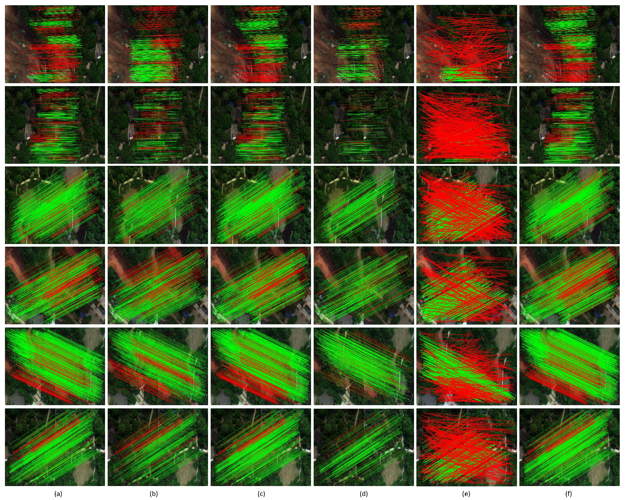
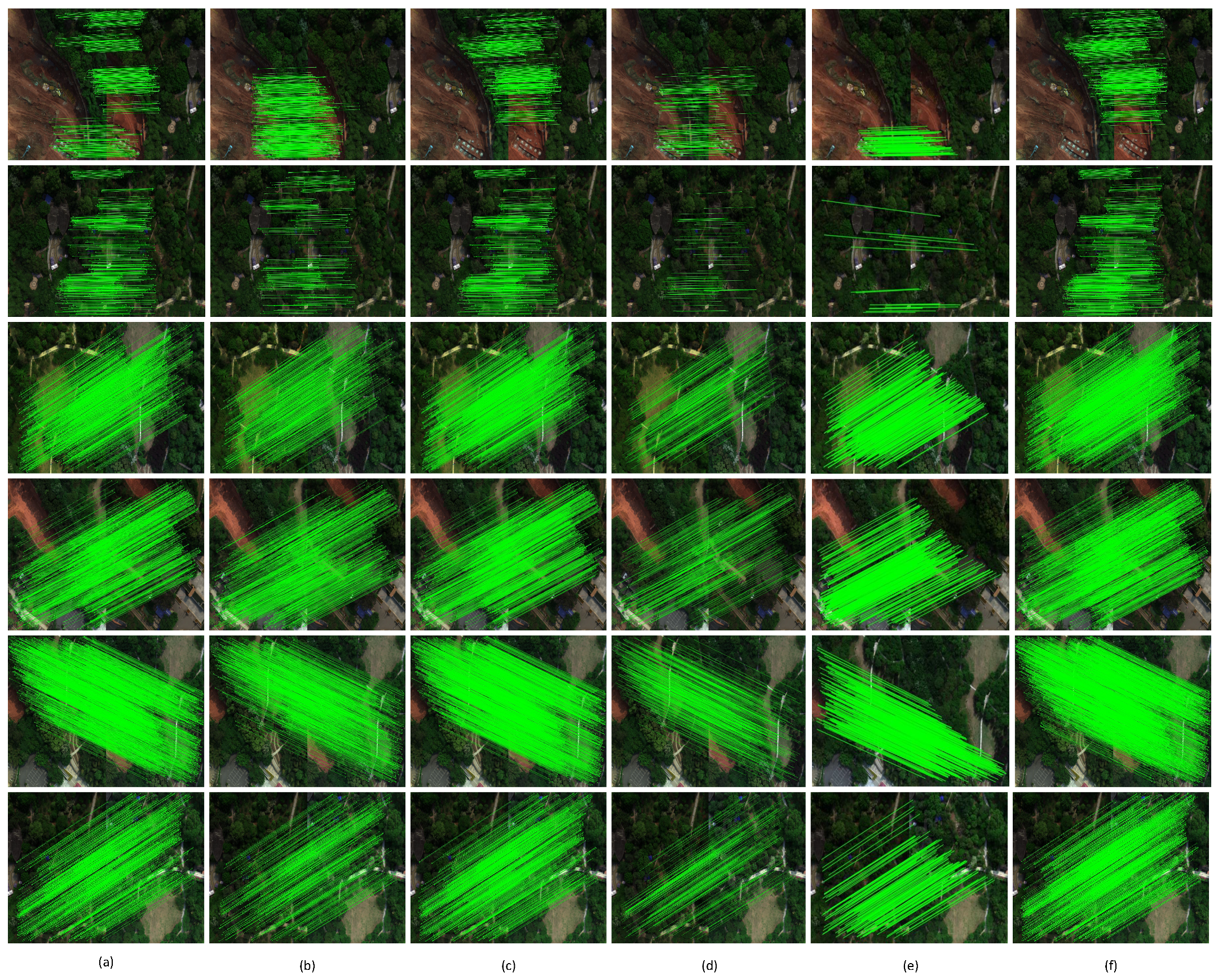
4.3.1. Detected Feature Points of Putative Matching Results

The putative matching results of SIFT, SURF, ROOT-SIFT, 3D-SIFT, SS-SIFT and HOSG-SIFT on UAV images are shown in Figure 8. We also count the number of detected feature points, putative matches and inliers as listed in

Table 3. The number of detected points and matching point pairs.

Method	Number of Feature Points	Number of Matches	Number of Inliers	Number of Outliers	Ratio of Inliers (%)
SIFT	7162	710	553	157	77.99
SURF	7844	644	452	192	70.32
ROOT-SIFT	7162	780	614	166	78.61
3D-SIFT	5908	364	269	95	73.98
SS-SIFT	11,673	1107	431	676	38.97
HOSG-SIFT	7162	915	727	188	79.54

to compare the putative matching results of different methods clearly. The statistical results in Table 3 conform to the matching results in Figure 8.

Among the spatial descriptors, ROOT-SIFT, as an improved version from SIFT, does the best with the matches number of 780 and the inliers number of 614. However, the keypoints with similar spatial structures are falsely regarded as matching point pairs since the spatial descriptors are designed for gray scales images without considering the spectral feature of objects.

3D-SIFT pictured in Figure 8d generates a minimun number of putative matches of 364 and inliers of 269 since it is proposed for medical image registration and performs relatively low when applied to HSI cube. By exploring both spectral and spatial dimensions simultaneously, SS-SIFT produces a largest number of putative matches but with a small number of inliers of 431, as shown in Figure 8e.

Compared with the methods mentioned above, HOSG-SIFT pictured in Figure 8f obtains a relatively high matches number and the largest inliers number. Different with SS-SIFT, we use a HOSG instead of 3D HOG to combine the spatial feature and spectral feature. Using spectral feature increases the number of putative matches. On the other hand, spectral profile is completely preserved by using the HOSG, thus the number of outliers (wrong matches) is decreased. Consequently, our method generates more high-quality putative matches with fewer outliers, demonstrating the effectiveness of the spectral feature in HSI matching tasks.

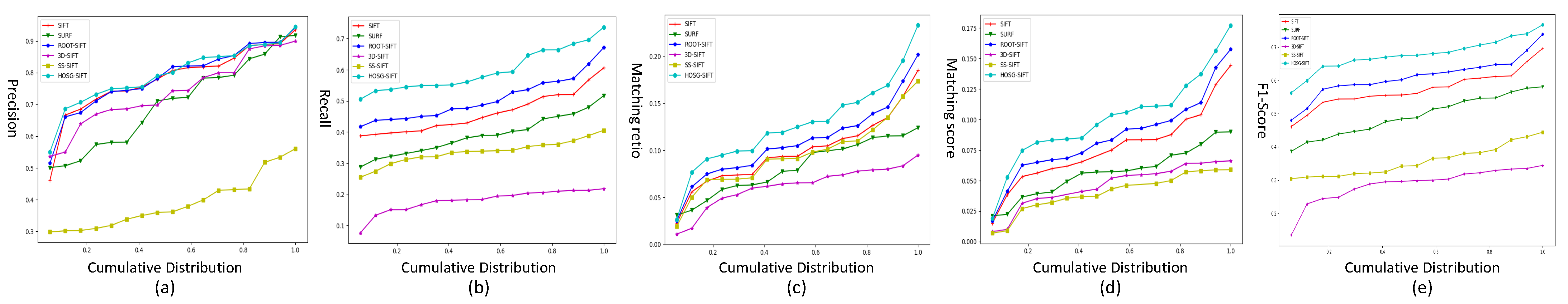
4.3.2. Evaluation Metrics of Putative Matching Results

The Quantitative evaluation metrics are summarized in Figure 9 by precision, recall, matching ratio and matching score with cumulative distribution. Moreover, the average values of each evaluations is demonstrated in

Table 4. Quantitative performance of methods on UAV dataset.

Method	Precision	Recall	Matching Ratio	Matching Score	F1-Score
SIFT	77.99	46.19	9.92	7.74	57.37
SURF	70.32	38.98	8.21	5.66	49.39
ROOT-SIFT	78.61	50.73	10.90	8.59	61.10
3D-SIFT	73.98	18.01	6.17	4.59	28.77
SS-SIFT	38.97	33.61	9.48	3.69	35.71
HOSG-SIFT	79.54	59.87	12.77	10.10	67.77

for a more straightforward and comprehensive comparison.

Regarding the spatial descriptors, it is hard to distinguish those false matches with similar spatial features due to the lack of spectral information. Among them, ROOT-SIFT achieves superior results of the highest precision and the best recall due to the benefits of using a square root kernel instead of the standard Euclidean distance to measure the similarity. SURF is designed to accelerate SIFT and improve matching efficiency, which is sensitive to viewpoint and illumination. Therefore, regarding UAV HSIs where the viewpoint and illumination change frequently, SURF obtains inferior results in matching tasks compared with SIFT and ROOT-SIFT.

On the contrary, the evaluation results of 3D descriptors, including 3D-SIFT and SS-SIFT, are relatively poor, same as the results in Figure 8 and Table 3. 3D-SIFT is usually used for medical image processing with an outstanding performance. Medical image is structurally different from HSI, whose pixels in different slices represent different spatial locations. Thus, 3D-SIFT is limited in HSI matching. Additionally, SS-SIFT takes advantage of spatial and spectral features by 3D HOG. In this way, the falsely extracted matches increase along with the number of putative matches result in a deficient performance of SS-SIFT.

By comparison, the proposed method obtains a considerable precision of 79.54%, a recall of 59.87%, and the best F1-score of 67.77%. Our descriptor outperforms the spatial descriptors since we simultaneously explore the spatial and spectral information, which are essential to distinguish objects with similar spatial features but different spectral features. On the other hand, our approach also surpasses the performance of 3D descriptors, telling that extracting the HOSG to describe spectral features is effective and robust.

4.3.3. Matching Results from RANSAC

As shown in Figure 8 the putative matches contain a lot of outliers inevitably [50,51]. Using outlier filtering algorithms to improve the performance of image matching is commonly used. Here, we use RANSAC to remove outliers in the experiments and evaluate the descriptors in matching tasks.

The matching results by RANSAC filtering are shown in Figure 10. Most outliers are erased by the RANSAC algorithm. However, the number and ratio of outliers in putative matching significantly impact the performance of RANSAC. Although RANSAC improves the SS-SIFT results to a large extent, the performance of SS-SIFT is still limited due to numerous outliers in putative matching. Fewer matching pairs are preserved and distribute unevenly (see the first and second figures in Figure 10e. Regarding 3D-SIFT, a part of outliers is removed in putative matching results. Thus, fewer matching pairs are preserved after outliers filtering.

By comparison, our method produces densely correct matches distributed evenly across the image after outliers filtering, exceeding the performance of other conventional methods pictured in Figure 10. The results generated by RANSAC also demonstrate that the feasibility of the proposed method.

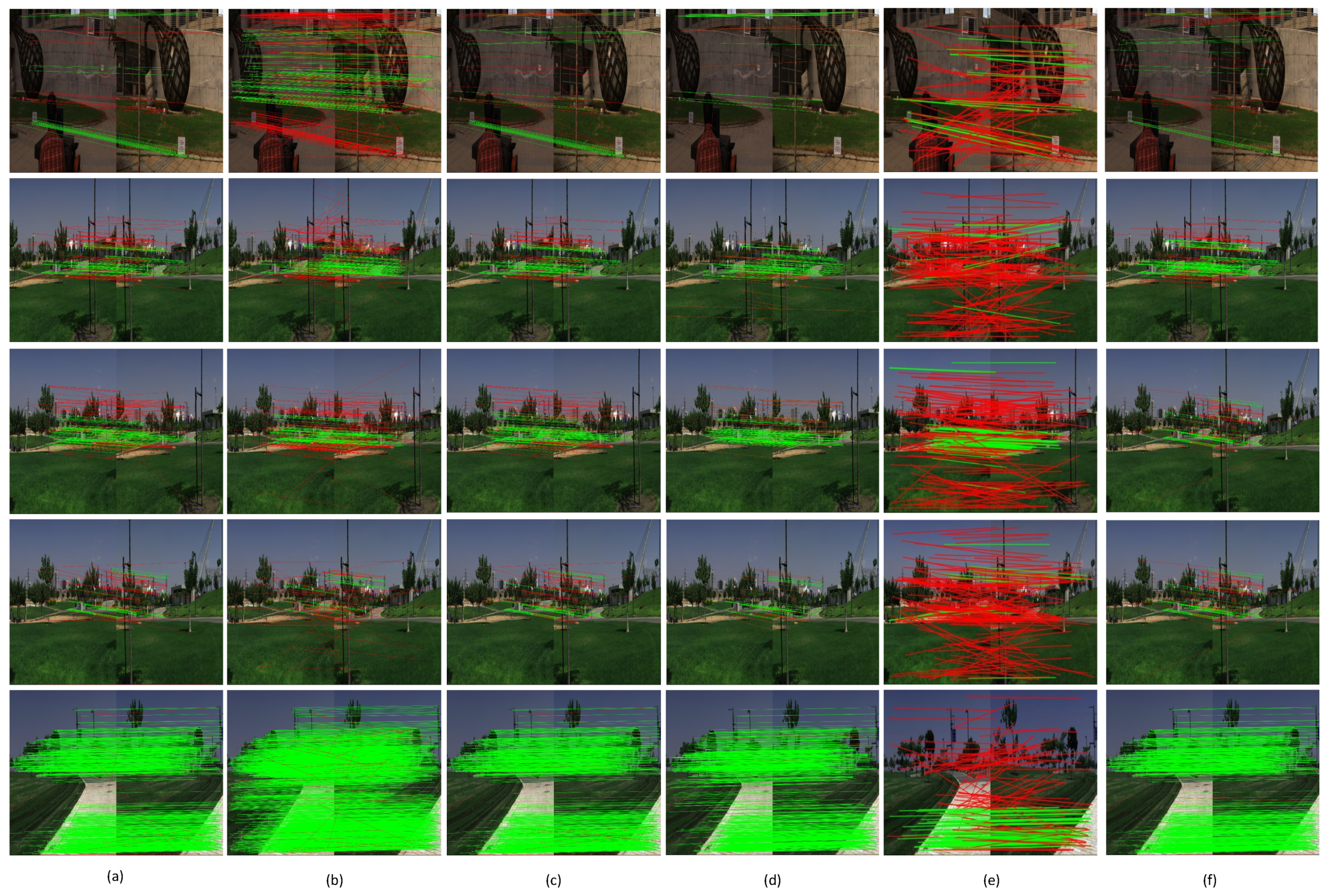
4.4. Matching Results on ICVL Dataset

To verify the robustness of our method, we also compare matching ability on the ICVL dataset collected by the ground platform. The ground platform HSIs are usually used for spectral reconstruction, thus there is no ground truth of the dataset for matching evaluation. Considering such a situation, we apply the RANSAC algorithm to estimate the homography and regard the results as the transformation matrix of images. The putative matching results of ground platform HSIs are shown in Figure 11. The quantitative metrics are listed in

Table 5. Quantitative performance of six methods on ICVL dataset.

Method	Precision	Recall	Matching Ratio	Matching Score	F1-Score
SIFT	45.98	56.71	9.15	6.23	50.35
SURF	41.50	78.93	14.33	9.55	53.95
ROOT-SIFT	47.12	57.66	10.11	6.99	51.30
3D-SIFT	43.78	45.33	5.18	3.29	44.19
SS-SIFT	23.97	37.45	4.41	2.17	29.32
HOSG-SIFT	49.08	60.68	11.52	7.87	53.72

.

Similar to the matching results of UAV HSIs, ROOT-SIFT obtains a precision of 47.12% that is higher than SIFT and SURF but poorer than our method, whose precision is 49.08%. The matching results of descriptors are depressed without considering the benefits spectral features. SURF produces a large amount of putative matching, and receives the best recall of 78.93% that is higher than our method by 18.25%.

Due to the limits of algorithms, matching errors prevalently exist. Although 3D-SIFT pictured in Figure 11d eliminates some false matches by taking advantage of multiband information, the putative matching number of 3D-SIFT results decrease along with the errors. Similarly, SS-SIFT shows the inferior performance on evaluation metrics since it requires outliers filtering for enhancement.

By contrast, our method outperforms other methods with more correct matches while preserving the precision, as depicted in Figure 11f. The matching results in the ICVL dataset also reveal that the robustness and effectiveness of proposed method.

4.5. Running Time Comparison

We compare the running time of different methods, as shown in

Table 6. Average running time(s).

Method	UAV	ICVL
SIFT	8.7	1.1
SURF	4.1	1.7
ROOT-SIFT	9.2	1.6
3D-SIFT	1917.5	88.2
SS-SIFT	2354.9	105.2
HOSG-SIFT	305.8	17.9

. Without considering the spectral feature, spatial descriptors perform more effective than 3D descriptors. In other words, constructing a descriptor based on multiple dimensions features is much more time-consuming. SURF operates fastest since it simplifies the extracting process by using the Hessian matrix instead of DOG to detect key points. In addition, ROOT-SIFT yields a relatively good performance without increasing computational costs.

3D descriptors, including 3D-SIFT and SS-SIFT, cost much time in keypoints detection and descriptors construction as they use 3D Gaussian convolution kernel and 3D-DOG to generate spatial-spectral keypoints. Although our descriptor is less effective than spatial descriptors, we get higher results both in precision and recall. We also learn that considering the spatial and spectral features both will increase the computing time. On the other hand, compared with existed 3D descriptors, our approach, constructing a HOSG profile in surrounding neighbors, is much more time-saving and performs more outstanding.

5. Discussion

The proposed method to construct HSI descriptors has three main steps: spatial descriptor extraction from grayscale images, spectral descriptor generation using HOSG and spatial-spectral descriptor construction. Although HSI descriptors perform well in HSI matching, limitations still exist.

On the one hand, regarding the spatial and spectral features, they have the same weights in our spatial-spectral descriptor. We concatenate the spatial descriptor of 128 elements and the spectral descriptor of 128 elements to obtain a spatial-spectral descriptor of 256 elements. Generally, the weights of spatial and spectral features are supposed to vary in different scenarios. Although we verify the performance of the descriptor with fixed ratio of weights, we have yet to discuss this with the adaptive ratio of weights.

On the other hand, although our descriptor outperforms the common spatial descriptors in precision for HSI matching, our method is limited in efficiency since the spectral information increases the computing complexity. On the other hand, compared with 3D descriptors such as 3D-SIFT and SS-SIFT, our descriptor is superior as we apply the HOSG to present spectral features. Thus, we believe our method is an alternative for those cases without a request for very high efficiency.

6. Conclusions

This paper presents an HSI descriptor constructed using SIFT and HOSG, which combines spatial and spectral features. The proposed HSI descriptors improve the performance of HSI matching with a precision of 79.54% in the UAV dataset and 49.80% in the ground platform dataset. In terms of overall performance, the proposed method outperforms other popular descriptors. Moreover, compared to spatial descriptors, the proposed method can better distinguish objects with the same material but different structures, providing a reference for descriptor construction in HSI. Considering the limitations of our work, we will enrich the diversity of hyperspectral image datasets in the future. Meanwhile, we will develop better feature extractors and matches with fewer errors using spectral information.

References

1. Adão, T.; Hruška, J.; Pádua, L.; Bessa, J.; Peres, E.; Morais, R.; Sousa, J.J. Hyperspectral imaging: A review on UAV-based sensors, data processing and applications for agriculture and forestry. Remote Sens. 2017, 9, 1110. [Google Scholar] [CrossRef] [Green Version]
2. Fu, Y.; Yang, G.; Song, X.; Li, Z.; Xu, X.; Feng, H.; Zhao, C. Improved estimation of winter wheat aboveground biomass using multiscale textures extracted from UAV-based digital images and hyperspectral feature analysis. Remote Sens. 2021, 13, 581. [Google Scholar] [CrossRef]
3. Guo, A.; Huang, W.; Dong, Y.; Ye, H.; Ma, H.; Liu, B.; Wu, W.; Ren, Y.; Ruan, C.; Geng, Y. Wheat yellow rust detection using UAV-based hyperspectral technology. Remote Sens. 2021, 13, 123. [Google Scholar] [CrossRef]
4. Thenkabail, P.S.; Smith, R.B.; De Pauw, E. Hyperspectral vegetation indices and their relationships with agricultural crop characteristics. Remote Sens. Environ. 2000, 71, 158–182. [Google Scholar] [CrossRef]
5. Wu, J.L.; Ho, C.R.; Huang, C.C.; Srivastav, A.L.; Tzeng, J.H.; Lin, Y.T. Hyperspectral sensing for turbid water quality monitoring in freshwater rivers: Empirical relationship between reflectance and turbidity and total solids. Sensors 2014, 14, 22670–22688. [Google Scholar] [CrossRef] [PubMed] [Green Version]
6. Gao, L.; Yao, D.; Li, Q.; Zhuang, L.; Zhang, B.; Bioucas-Dias, J.M. A new low-rank representation based hyperspectral image denoising method for mineral mapping. Remote Sens. 2017, 9, 1145. [Google Scholar] [CrossRef] [Green Version]
7. Feng, Y.Z.; Sun, D.W. Application of hyperspectral imaging in food safety inspection and control: A review. Crit. Rev. Food Sci. Nutr. 2012, 52, 1039–1058. [Google Scholar] [CrossRef]
8. Lu, G.; Fei, B. Medical hyperspectral imaging: A review. J. Biomed. Opt. 2014, 19, 010901. [Google Scholar] [CrossRef]
9. Schonberger, J.L.; Hardmeier, H.; Sattler, T.; Pollefeys, M. Comparative evaluation of hand-crafted and learned local features. In Proceedings of the IEEE Conference on Computer Vision and Pattern Recognition, Honolulu, HI, USA, 21–26 July 2017; pp. 1482–1491. [Google Scholar]
10. Ma, J.; Ye, X.; Zhou, H.; Mei, X.; Fan, F. Loop-Closure Detection Using Local Relative Orientation Matching. IEEE Trans. Intell. Transp. Syst. 2021, 1–14. [Google Scholar] [CrossRef]
11. Li, J.; Wang, Z.; Lai, S.; Zhai, Y.; Zhang, M. Parallax-tolerant image stitching based on robust elastic warping. IEEE Trans. Multimed. 2017, 20, 1672–1687. [Google Scholar] [CrossRef]
12. Lee, K.Y.; Sim, J.Y. Warping residual based image stitching for large parallax. In Proceedings of the IEEE/CVF Conference on Computer Vision and Pattern Recognition, Seattle, WA, USA, 13–19 June 2020; pp. 8198–8206. [Google Scholar]
13. Yang, Y.; Lee, X. Four-band thermal mosaicking: A new method to process infrared thermal imagery of urban landscapes from UAV flights. Remote Sens. 2019, 11, 1365. [Google Scholar] [CrossRef] [Green Version]
14. Zhang, H.; Xu, H.; Tian, X.; Jiang, J.; Ma, J. Image fusion meets deep learning: A survey and perspective. Inf. Fusion 2021, 76, 323–336. [Google Scholar] [CrossRef]
15. Xu, H.; Ma, J.; Jiang, J.; Guo, X.; Ling, H. U2Fusion: A unified unsupervised image fusion network. IEEE Trans. Pattern Anal. Mach. Intell. 2020. [Google Scholar] [CrossRef]
16. Nesbit, P.R.; Hugenholtz, C.H. Enhancing UAV–SFM 3D model accuracy in high-relief landscapes by incorporating oblique images. Remote Sens. 2019, 11, 239. [Google Scholar] [CrossRef] [Green Version]
17. Jiang, S.; Jiang, C.; Jiang, W. Efficient structure from motion for large-scale UAV images: A review and a comparison of SfM tools. ISPRS J. Photogramm. Remote Sens. 2020, 167, 230–251. [Google Scholar] [CrossRef]
18. Meinen, B.U.; Robinson, D.T. Mapping erosion and deposition in an agricultural landscape: Optimization of UAV image acquisition schemes for SfM-MVS. Remote Sens. Environ. 2020, 239, 111666. [Google Scholar] [CrossRef]
19. Sattler, T.; Leibe, B.; Kobbelt, L. Fast image-based localization using direct 2d-to-3d matching. In Proceedings of the 2011 International Conference on Computer Vision, Barcelona, Spain, 6–13 November 2011; pp. 667–674. [Google Scholar]
20. Sattler, T.; Leibe, B.; Kobbelt, L. Efficient & effective prioritized matching for large-scale image-based localization. IEEE Trans. Pattern Anal. Mach. Intell. 2016, 39, 1744–1756. [Google Scholar]
21. Zia, A.; Zhou, J.; Gao, Y. Exploring Chromatic Aberration and Defocus Blur for Relative Depth Estimation From Monocular Hyperspectral Image. IEEE Trans. Image Process. 2021, 30, 4357–4370. [Google Scholar] [CrossRef] [PubMed]
22. Luo, B.; Chanussot, J. Hyperspectral image classification based on spectral and geometrical features. In Proceedings of the 2009 IEEE International Workshop on Machine Learning for Signal Processing, Grenoble, France, 1–4 September 2009; pp. 1–6. [Google Scholar]
23. Lu, B.; Dao, P.D.; Liu, J.; He, Y.; Shang, J. Recent advances of hyperspectral imaging technology and applications in agriculture. Remote Sens. 2020, 12, 2659. [Google Scholar] [CrossRef]
24. Allaire, S.; Kim, J.J.; Breen, S.L.; Jaffray, D.A.; Pekar, V. Full orientation invariance and improved feature selectivity of 3D SIFT with application to medical image analysis. In Proceedings of the 2008 IEEE Computer Society Conference on Computer Vision and Pattern Recognition Workshops, Anchorage, AK, USA, 23–28 June 2008; pp. 1–8. [Google Scholar]
25. Tsai, F.; Lai, J.S. Feature extraction of hyperspectral image cubes using three-dimensional gray-level cooccurrence. IEEE Trans. Geosci. Remote Sens. 2013, 51, 3504–3513. [Google Scholar] [CrossRef]
26. Tang, Y.Y.; Lu, Y.; Yuan, H. Hyperspectral image classification based on three-dimensional scattering wavelet transform. IEEE Trans. Geosci. Remote Sens. 2014, 53, 2467–2480. [Google Scholar] [CrossRef]
27. Everts, I.; Van Gemert, J.C.; Gevers, T. Evaluation of color spatio-temporal interest points for human action recognition. IEEE Trans. Image Process. 2014, 23, 1569–1580. [Google Scholar] [CrossRef] [Green Version]
28. Al-Khafaji, S.L.; Zhou, J.; Zia, A.; Liew, A.W.C. Spectral-spatial scale invariant feature transform for hyperspectral images. IEEE Trans. Image Process. 2017, 27, 837–850. [Google Scholar] [CrossRef] [PubMed] [Green Version]
29. Ma, J.; Jiang, X.; Fan, A.; Jiang, J.; Yan, J. Image matching from handcrafted to deep features: A survey. Int. J. Comput. Vis. 2021, 129, 23–79. [Google Scholar] [CrossRef]
30. Lowe, D.G. Distinctive image features from scale-invariant keypoints. Int. J. Comput. Vis. 2004, 60, 91–110. [Google Scholar] [CrossRef]
31. Bay, H.; Ess, A.; Tuytelaars, T.; Van Gool, L. Speeded-up robust features (SURF). Comput. Vis. Image Underst. 2008, 110, 346–359. [Google Scholar] [CrossRef]
32. Arandjelović, R.; Zisserman, A. Three things everyone should know to improve object retrieval. In Proceedings of the 2012 IEEE Conference on Computer Vision and Pattern Recognition, Providence, RI, USA, 16–21 June 2012; pp. 2911–2918. [Google Scholar]
33. Ke, Y.; Sukthankar, R. PCA-SIFT: A more distinctive representation for local image descriptors. In Proceedings of the 2004 IEEE Computer Society Conference on Computer Vision and Pattern Recognition, Washington, DC, USA, 27 June–2 July 2004; Volume 2, p. II-II. [Google Scholar]
34. Dong, J.; Soatto, S. Domain-size pooling in local descriptors: DSP-SIFT. In Proceedings of the IEEE Conference on Computer Vision and Pattern Recognition, Boston, MA, USA, 7–12 June 2015; pp. 5097–5106. [Google Scholar]
35. Yi, K.M.; Trulls, E.; Lepetit, V.; Fua, P. Lift: Learned invariant feature transform. In European Conference on Computer Vision; Springer: Berlin/Heidelberg, Germany, 2016; pp. 467–483. [Google Scholar]
36. Barroso-Laguna, A.; Riba, E.; Ponsa, D.; Mikolajczyk, K. Key. net: Keypoint detection by handcrafted and learned cnn filters. In Proceedings of the IEEE/CVF International Conference on Computer Vision, Long Beach, CA, USA, 16–17 June 2019; pp. 5836–5844. [Google Scholar]
37. DeTone, D.; Malisiewicz, T.; Rabinovich, A. Superpoint: Self-supervised interest point detection and description. In Proceedings of the IEEE Conference on Computer Vision and Pattern Recognition Workshops, Salt Lake City, UT, USA, 18–22 June 2018; pp. 224–236. [Google Scholar]
38. Mishchuk, A.; Mishkin, D.; Radenovic, F.; Matas, J. Working hard to know your neighbor’s margins: Local descriptor learning loss. arXiv 2017, arXiv:1705.10872. [Google Scholar]
39. Jiang, X.; Ma, J.; Xiao, G.; Shao, Z.; Guo, X. A review of multimodal image matching: Methods and applications. Inf. Fusion 2021, 73, 22–71. [Google Scholar] [CrossRef]
40. Cheung, W.; Hamarneh, G. n-SIFT: n-Dimensional Scale Invariant Feature Transform. IEEE Trans. Image Process. 2009, 18, 2012–2021. [Google Scholar] [CrossRef] [Green Version]
41. Scovanner, P.; Ali, S.; Shah, M. A 3-dimensional sift descriptor and its application to action recognition. In Proceedings of the 15th ACM International Conference on Multimedia, New York, NY, USA, 24–29 September 2007; pp. 357–360. [Google Scholar]
42. Rister, B.; Horowitz, M.A.; Rubin, D.L. Volumetric image registration from invariant keypoints. IEEE Trans. Image Process. 2017, 26, 4900–4910. [Google Scholar] [CrossRef]
43. Dorado-Munoz, L.P.; Velez-Reyes, M.; Mukherjee, A.; Roysam, B. A vector SIFT detector for interest point detection in hyperspectral imagery. IEEE Trans. Geosci. Remote Sens. 2012, 50, 4521–4533. [Google Scholar] [CrossRef]
44. Angelopoulou, E.; Lee, S.W.; Bajcsy, R. Spectral gradient: A material descriptor invariant to geometry and incident illumination. In Proceedings of the Seventh IEEE International Conference on Computer Vision, Corfu, Greece, 20–27 September 1999; Volume 2, pp. 861–867. [Google Scholar]
45. Wold, S.; Esbensen, K.; Geladi, P. Principal component analysis. Chemom. Intell. Lab. Syst. 1987, 2, 37–52. [Google Scholar] [CrossRef]
46. Arad, B.; Ben-Shahar, O. Sparse Recovery of Hyperspectral Signal from Natural RGB Images. In European Conference on Computer Vision; Springer: Cham, Switzerland, 2016; pp. 19–34. [Google Scholar]
47. Jin, Y.; Mishkin, D.; Mishchuk, A.; Matas, J.; Fua, P.; Yi, K.M.; Trulls, E. Image matching across wide baselines: From paper to practice. Int. J. Comput. Vis. 2021, 129, 517–547. [Google Scholar] [CrossRef]
48. Zhang, Y.; Wang, J.; Xu, S.; Liu, X.; Zhang, X. MLIFeat: Multi-level information fusion based deep local features. In Proceedings of the Asian Conference on Computer Vision, Kyoto, Japan, 30 November–4 December 2020. [Google Scholar]
49. Fischler, M.A.; Bolles, R.C. Random sample consensus: A paradigm for model fitting with applications to image analysis and automated cartography. Commun. ACM 1981, 24, 381–395. [Google Scholar] [CrossRef]
50. Ma, J.; Zhao, J.; Jiang, J.; Zhou, H.; Guo, X. Locality preserving matching. Int. J. Comput. Vis. 2019, 127, 512–531. [Google Scholar] [CrossRef]
51. Ma, J.; Jiang, X.; Jiang, J.; Zhao, J.; Guo, X. LMR: Learning a two-class classifier for mismatch removal. IEEE Trans. Image Process. 2019, 28, 4045–4059. [Google Scholar] [CrossRef] [PubMed]
Figure 1. Overall framework of HOSG-SIFT construction. The spatial-spectral descriptor of 256 elements is constructed by concatenating the spatial and spectral descriptor. The weights of the spatial and spectral descriptor are w 1 and w 2 , respectively. In this paper, we use the same w 1 and w 2 .
Remotesensing 13 04912 g001
Figure 2. A comparision: extracting the spatial interest points from single band image (red, green and blue band) and the first principal component of HSI generated by PCA. Figures (ac) depict the spatial interest points extracted from red, green, and blue band, respectively. Figure (d) shows the spatial interest points extracted from the first principal component of HSI, which is generated using PCA.
Remotesensing 13 04912 g002
Figure 3. Spatial descriptor construction using the histogram of gradient. The image sample points are then accumulated into 8 orientation histograms summarizing the contents over 4 × sub-regions. Therefore, a 8 × 4 × 4 elements spatial feature vector is constructed for each keypoint.
Remotesensing 13 04912 g003
Figure 4. The difference of original spectral profile and spectral gradient profile. Figure (a) represents the RGB image synthesized by selecting the red, green and blue bands. We select two points A and B for comparison. Figure (b) and Figure (c) show the original spectral profile of point A and B, respectively. Figure (d) and Figure (e) are the spectral gradient profile of point A and B, respectively.
Remotesensing 13 04912 g004
Figure 5. The pipeline of the spectral descriptor construction. A patch with the size of 16 × 16 × n is first designated surrounding the centre of each keypoint. Then the patch is split up regularly into 16 sub-regions with the size of 4 × 4 × n . We extract the spectral gradient histogram for each sub-region. Finally, the spectral gradient histogram of 16 sub-regions are concatenated to construct the spectral descriptor of 128 elements.
Remotesensing 13 04912 g005
Figure 6. Extracting the HOSG of the sub-region.
Remotesensing 13 04912 g006
Figure 7. Parameters Testing. Figure (a) shows the performance of the spatial-spectral descriptor with the different weights of the spatial and spectral feature vector. The results tell that the spatial and spectral descriptor are equally important for HSI feature representation. Figure (b) shows that the number of sub-regions and vertices affect the performance of the descriptor. The spatial-spectral descriptor performs the best with 16 sub-regions and eight vertices.
Remotesensing 13 04912 g007
Figure 8. Putative Matching Results. (af) represent the putative matching result of SIFT, SURF, ROOT-SIFT, 3D-SIFT, SS-SIFT, and HOSG-SIFT respectively. The green lines present inliers while the red lines are outliers.
Remotesensing 13 04912 g008
Figure 9. Cumulative distribution of precision, recall, matching ratio, matching score and F1-score. Figures (ae) are the cumulative distribution of precision, recall, matching ratio, matching score, and F1-score, respectively. A point on the curve with coordinate (x,y) denotes that there are (100 × x) percents of image pairs which have the performance value no more than y.
Remotesensing 13 04912 g009
Figure 10. Matching Results using RANSAC. (af) represent the matching result of SURF, SIFT, ROOT-SIFT, 3D-SIFT, SS-SIFT, and HOSG-SIFT method respectively.
Remotesensing 13 04912 g010
Figure 11. Putative Matching Results of ground platform HSIs. (af) represent the putative matching result of SIFT, SURF, ROOT-SIFT, 3D-SIFT, SS-SIFT, and our method respectively. The green lines present inliers while the red lines are outliers.
Remotesensing 13 04912 g011