Change Detection for Heterogeneous Remote Sensing Images with Improved Training of Hierarchical Extreme Learning Machine (HELM)

Abstract

To solve the problems of susceptibility to image noise, subjectivity of training sample selection, and inefficiency of state-of-the-art change detection methods with heterogeneous images, this study proposes a post-classification change detection method for heterogeneous images with improved training of hierarchical extreme learning machine (HELM). After smoothing the images to suppress noise, a sample selection method is defined to train the HELM for each image, in which the feature extraction is respectively implemented for heterogeneous images and the parameters need not be fine-tuned. Then, the multi-temporal feature maps extracted from the trained HELM are segmented to obtain classification maps and then compared to generate a change map with changed types. The proposed method is validated experimentally by using one set of synthetic aperture radar (SAR) images obtained from Sentinel-1, one set of optical images acquired from Google Earth, and two sets of heterogeneous SAR and optical images. The results show that compared to state-of-the-art change detection methods, the proposed method can improve the accuracy of change detection by more than 8% in terms of the kappa coefficient and greatly reduce run time regardless of the type of images used. Such enhancement reflects the robustness and superiority of the proposed method.

1. Introduction

Change detection intends to identify the changes between a given image pair of the same scene acquired at different times [1]. With the advancement of remote sensing technology, remote sensing data have developed into multi-temporal, multi-channel, and multi-source data that serve as the main source for detecting changes on the Earth’s surface. Change detection is widely used with various types of remote sensing data (e.g., synthetic aperture radar (SAR), optical, light detection and ranging (LiDAR), and geographic information system (GIS) data) in many fields, such as land cover monitoring [2], forest cover monitoring [3], and disaster assessment [4]. According to the characteristics of multi-temporal images, change detection methods can be divided into change detection with homogeneous or heterogeneous images.

In change detection with homogeneous images, the multi-temporal images used for change detection are acquired from the same remote sensing sensor. Numerous methods have been proposed for change detection with homogeneous images. According to processing units, these change detection methods can be divided into pixel-based and object-based ones. Pixel-based methods generally generate a difference map (DM) through a pixel-by-pixel comparison of multi-temporal image features and determine the changed and unchanged regions through the analysis of the DM. Many algorithms are used to analyze DM, and they include thresholding algorithms (e.g., Otsu [5], Minimum error thresholding algorithm [6], change vector analysis (CVA) [7]), clustering algorithms (e.g., fuzzy c-means (FCM) [8], principal component analysis and k-means clustering (PCA-kmeans) [9], fuzzy local information C-means (FLICM) [10]), and algorithms for optimizing criterion functions (e.g., genetic algorithm (GA) [11], particle swarm optimization (PSO) [12], Markov random fields (MRF) [13], slow feature analysis (SFA) [14]). However, because of the lack of spatial and contextual information of images, pixel-based methods are susceptible to “salt–pepper noise.”

In recent years, a large number of object-based change detection methods have been proposed [15,16,17,18] to detect changed objects with spatially adjacent and spectrally similar pixels on the basis of the human visual mechanism [19]. Object-based methods utilize image objects’ features (e.g., size, shape, structure, texture, spectrum) for multi-temporal comparison and thus make up for the limitation of pixel-based methods that only consider pixel spectra [20,21]. Nevertheless, the effectiveness of object-based methods depends on the quality of image segmentation.

With the development of neural networks, several deep learning (DL)-based change detection methods with homogeneous images, such as PCANet [22], multiscale CapsNet (Ms-CapsNet) [23], convolutional wavelet neural network (CWNN) [24] and deep slow feature analysis (DSFA) [25] have been proposed, but they are not applicable to change detection with heterogeneous images.

In change detection with heterogeneous images, the images used are acquired by different remote sensing sensors, such as SAR, optical sensors, LIDAR, and GIS [26,27,28]. As optical images have extensive coverage and abundant spectra while SAR data provide all-weather and all-time observations, the current work focuses on change detection with optical and SAR images for application to emergency response, e.g., earthquakes, floods, volcanic eruptions, or forest fires. Given the considerable differences in data descriptions between SAR and optical images, change detection methods with homogeneous images are no longer applicable.

Compared to change detection with homogeneous images, change detection methods with heterogeneous images are currently in the development stage. They are divided into supervised and unsupervised types according to the automaticity involved in collecting training data. In supervised methods, Mercier et al. [28] assumed that the unchanged regions in two images are independent and estimated the local statistical relationship between the unchanged regions of the heterogeneous images by using Copulas theory according to the training samples that were manually selected; then, they performed a Kullback–Leibler-based comparison of the statistics to extract the change information. In [29], the homogeneous pixel transformation (HPT) technique was used to generate simulated optical and SAR images by manually selecting training samples of unchanged regions, and the changed regions were determined by comparing the simulated and original images. To reduce the reliance on training data, Alberga et al. compared the mutual information, cluster reward algorithm, and other similar measures for unsupervised change detection with heterogeneous images with certain windows [30]. An energy model was proposed in [31] to estimate the similarity map with FastMap-based optimization. These methods can roughly highlight changed regions, but they are sensitive to image noise and are prone to errors. Sun et al. also proposed a nonlocal patch similarity based graph (NPSG) [32] and improved NPSG (INLPG) [33] to measure the structure differences between heterogeneous images. However, the parameters of these methods need to be finely tuned.

With its superiority in terms of learning of training samples, machine learning is increasingly used in remote sensing change detection. A symmetric coupling convolutional network (SCCN) was proposed in [34], in which two heterogeneous images were transformed into the same feature space for comparison by training them with unchanged pixels. To enlarge the difference between changed and unchanged regions, the work in [35] proposed an approximately symmetrical deep neural network (ASDNN), which transforms heterogeneous images into common feature spaces and then highlights the changed regions by training them with changed and unchanged labels. To perform joint feature extraction on transformed SAR and optical images for the selection of training labels, the work in [36] proposed a logarithmic transformation feature learning (LTFL) framework and obtained the change map by using the trained classifier. Niu et al. used conditional generative adversarial network (CGAN) [37] to transform heterogeneous images into the same feature space for comparison. All these methods could adequately learn training samples, but they are time consuming.

In this paper, to address the issue of image noise susceptibility and manual sample selection, and to take advantage of machine learning whiling improving algorithm efficiency, the current work proposes a change detection method with heterogeneous images that is based on hierarchical extreme learning machine classification (HELMC). Despite the vast variances in imaging characteristics in heterogeneous images, the same Ground objects may be represented by the same labels, and change information can be retrieved by comparing the labels.

In this method, SAR and optical images are first smoothed separately to reduce the effects of image noise. Then, a measurement between pixels and cluster centers is proposed for the automatic selection of training samples among the multi-temporal images. In training the hierarchical extreme learning machine (HELM), the hidden layers can use parameters that are given randomly without adjustment [38] to obtain meaningful feature representations and high learning efficiency. After the segmentation of the multi-temporal feature maps to obtain the classification maps, a change map is generated through the comparison of the multi-temporal classification maps. The main contributions of this work are summarized as follows:

(1)

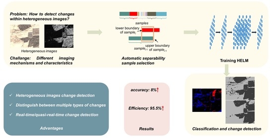
This paper proposes a new change detection framework, which is applicable to both homogeneous/heterogeneous images change detection, not only to obtain changed regions, but also to distinguish changed types.

(2)

This paper proposes a separable training sample selection method to train the network, which accurately selects training samples and does not need to utilize additional training datasets.

(3)

HELM with less parameter adjustment in network training is introduced for multi-temporal feature extraction to improve the accuracy and efficiency of change detection with heterogeneous images.

The rest of the paper is organized as follows: Section 2 introduces the related theories about HELM and describes HELMC in detail. Section 3 displays the experimental results for heterogeneous and homogeneous images. Section 4 discusses the paper. Section 5 provides the conclusion and future work directions.

2. Materials and Methods

2.1. HELM

HELM is a new hierarchical learning framework based on extreme learning machine (ELM) [39]. HELM has a deeper architecture than ELM and is thus able to achieve more meaningful features. As shown in Figure 1, HELM has two parts: (1) multilayer forward encoding and (2) original ELM.

2.1.1. Multilayer Forward Encoding

In the first part, HELM transforms data into an ELM random feature space to exploit any hidden layer information. The output of each hidden layer can be expressed as:

$$H_i=g\left(H_{i-1}·\mathit{\beta }\right)$$

(1)

where $\mathbf{\beta }$ is the hidden layer weight. $H_{i-1}$ and $H_i$ respectively represent the output matrix of the $i$th and $\left(i-1\right)$th $\left(i\in \left[1,K\right]\right)$ hidden layers. $g(·)$ is the activation function of the hidden layer. Through the multilayer forward encoding among hidden layers in the HELM framework, the parameters of the following hidden layer are determined as long as the features of the previous hidden layer are extracted.

Therefore, HELM has a higher computational efficiency than some traditional DL frameworks [40] that require parameter adjustment.

The hidden layer weights $\mathbf{\beta }$ can be optimized by an ELM sparse autoencoder to obtain good generalization and a fast learning speed.

$$O_{\mathbf{\beta }}=\arg \min \{{\Vert H_{i-1}\mathbf{\beta }-X\Vert }^2+{\Vert \mathbf{\beta }\Vert }_{l_1}\}$$

(2)

where $X$ is the training set and $l_1$ is a constraint term.

2.1.2. Original ELM

In the second part, the final output $F$ is obtained on the basis of the original ELM [39], that is,

$$F=H_K\ast {\mathbf{\beta }}_{out}$$

(3)

where the output weight ${\mathbf{\beta }}_{out}$ is calculated by

$${\mathbf{\beta }}_{out}=H_K^T{\left(\frac{1}{\lambda }+H_K{H}_K^T\right)}^{-1}T$$

(4)

where $T$ is the target matrix and $\lambda$ is a positive value to improve the stability of ELM.

2.2. Methodology

Consider two co-registered heterogeneous images of a same scene, $I_1=\{I_1\left(i,j\right),1\le i\le H,1\le j\le W\}$ and $I_2=\{I_2\left(i,j\right),1\le i\le H,1\le j\le W\}$,which are acquired from SAR and optical sensors at different times $t_1$ and $t_2$, respectively. $H$ and $W$ are the height and width of each image, respectively. Figure 2 shows the proposed change detection framework for images $I_1$ and $I_2$ with HELMC. After smoothing images, HELM is trained by the proposed method for automatically selecting training samples separately from $I_1$ and $I_2$. Feature maps for each image are then generated. Then, the feature maps are segmented to obtain the multi-temporal classification maps, which are subsequently compared to identify changed regions and their categories.

To reduce the effect of image noise on change detection, this work applies the mean shift (MS) method [41] to the smoothening of the images according to their distribution without any prior information.

2.2.1. Training Sample Selection

The proposed selection of training samples is aimed toward the selection of pixels with values close to the cluster centers in a given smooth image. Given image $I\in [I_{\min },I_{\max }]$, where $I_{\min }$ and $I_{\max }$ respectively represent the minimum and maximum values of the image. The cluster centers of the smooth image are obtained by FCM [8], with the center values being $c_i$ ($i=1,2,\dots ,C$, and $c_i>c_{i-1}$), where $c$ represents the total number of image categories.

The objective function and constraints of the FCM are defined as

$$J={{\displaystyle \sum _{i=1}^c{\displaystyle \sum _{j=1}^n{u}_{ij}^m\Vert x_j-c_i\Vert }}}^2$$

(5)

$$\sum _{i=1}^c{u}_{ij}=1,j=1,2,\dots ,n$$

(6)

where m is the fuzzy factor of affiliation $u_{ij}$, $x_j$is the sample data, and n is the total number of samples in the dataset.

Each cluster center corresponds to a value interval of sample $sampl{e}_i$, and $\min \left(sampl{e}_i\right)<c_i<\max \left(sampl{e}_i\right),\left(i=1,2,\dots ,C\right)$, where $\min (·)$ and $\max (·)$ are the maximum and minimum operators, respectively. In this way, we have two cases: (1) the sample intervals do not overlap, and (2) the sample intervals overlap.

A schematic example is displayed in Figure 3 to illustrate the definition of the training sample selection. The case of the sample intervals not overlapping is shown in Figure 3a, which can be described as

$$\{\begin{array}{c}sampl{e}_1\in \left[I_{\min },t{h}_1\right]\\ sampl{e}_2\in \left[t{h}_1,t{h}_2\right]\\ ⋮\\ sampl{e}_{C-1}\in \left[t{h}_{C-2},t{h}_{C-1}\right]\\ sampl{e}_C\in \left[t{h}_{C-1},I_{\max }\right]\end{array}$$

(7)

where $t{h}_i\left(i=1,2,\dots ,C-1\right)$ represents the boundaries of the sample intervals, which are defined as

$$\{\begin{array}{l}t{h}_1=2c_1-I_{\min }\hfill \\ t{h}_i=2c_i-t{h}_{i-1},\left(i=1,2,\dots ,C-1\right)\hfill \\ t{h}_{C-1}=2c_C-I_{\max }\hfill \end{array}$$

(8)

where $I_{\min }<t{h}_{i-1}<t{h}_i<I_{\max }$.

As shown in Figure 3b, if the sample intervals overlap, then the upper boundary of $sampl{e}_{i-1}$ might be higher than the lower boundary of $sampl{e}_i$. This situation will cause the training samples are not pure enough, which will easily affect the image classification accuracy. In this condition, the values of boundaries $t{h}_i$ are defined as follows to improve the separability of the training samples:

$$\{\begin{array}{cc}t{h}_i=\frac{1}{2}\left(c_i+c_{i+1}\right),i=1,2,\dots ,C-1,& C>2\\ t{h}_1=t{h}_2=c_1+\frac{\left(c_1-I_{\min }\right)\left(c_2-c_1\right)}{I_{\max }-c_2+c_1-I_{\min }},& C=2\end{array}$$

(9)

2.2.2. Training of HELM

By attaching the cluster centers (target matrix $T$) to the training samples, the training sets $X$ are constructed to train HELM.

In multilayer forward encoding, the original data are converted to an ELM random space to extract the hidden layer features of the training samples. According to Equation (1), the output of each hidden layer is obtained. To obtain other sparse features and improve learning accuracy, this work uses an ELM sparse autoencoder in the optimization of the hidden layer weights according to Equation (2). In the original ELM, the universal approximation capability of ELM is used to obtain the output weight ${\mathbf{\beta }}_{out}$ according to Equation (4).

Each hidden layer of HELM is a separate feature extractor. Once the parameters of $O_{\mathbf{\beta }}$ and ${\mathbf{\beta }}_{out}$ in HELM are calculated, the training of HELM is completed.

2.2.3. Feature Map Generation

As the parameters of $O_{\mathbf{\beta }}$ and ${\mathbf{\beta }}_{out}$ in HELM are determined in the training process, the multi-temporal smooth images are separately used as inputs in the trained HELM to extract the feature maps. This process is similar to the training of HELM, and the hidden layer parameters used are obtained from the training of HELM. According to Equation (3), the final output is the feature map. The value of each category in the feature map is the value near the cluster center. Hence, the homogeneity of the same image category in the feature map is greater than that of the smooth image.

2.2.4. Change Detection Map Generation

The multi-temporal feature maps cannot be directly compared because their features are extracted from each image and they are unequal despite originating from the same category. Therefore, the FCM algorithm [8] is used to perform cluster analysis on the feature maps and mark the multi-temporal clusters with the same sets of category labels to generate comparable classification maps.

Subsequently, the change detection between the classification maps of $I_1$ and $I_2$ is carried out as

$$\{\begin{array}{cc}Cma{p}_{i.j}\left(I_1\right)-Cma{p}_{i.j}\left(I_2\right)=0,& unchanged\\ Cma{p}_{i.j}\left(I_1\right)-Cma{p}_{i.j}\left(I_2\right)\ne 0,& changed\end{array}$$

(10)

where $Cma{p}_{i.j}\left(I_1\right)$ and $Cma{p}_{i.j}\left(I_2\right)$ represent the category labels of pixel $(i,j)$ in the classification maps of $I_1$ and $I_2$, respectively.

In the changed regions, if the category labels of pixel $(i,j)$ in $Cma{p}_{i.j}\left(I_1\right)$ and $Cma{p}_{i.j}\left(I_2\right)$ are respectively “a” and “b”, then the changed type of pixel $(i,j)$ is “from a to b.”

3. Results

3.1. Dataset Description

To validate the proposed change detection method not only for heterogeneous images but also for homogeneous images, we used the following four datasets in the experiments: homogeneous SAR images, homogeneous optical images, and two sets of heterogeneous images acquired by SAR and optical sensors.

Figure 4 shows the homogeneous SAR images with a spatial resolution of 5 m and size of 1500 × 898 pixels. These images were acquired by the SAR sensor of Sentinel-1 satellite over a part of Yangtze River in China in November 2017 and May 2018. They reflected the changes in Yangtze River during this period.

Figure 5 shows the homogeneous optical images with a spatial resolution of 0.23 m and size of 774 × 372 pixels. The images were acquired from Google Earth in May 2009 and April 2014 and covered the same scene of a farmland in Wanghong town of China. They showed the changes in the wheat fields in this area.

Figure 6 and Figure 7 show the two sets of heterogeneous images acquired by optical and SAR sensors over another part of Yangtze River and a desert area in Guazhou County of China, respectively. The images measured 600 × 600 pixels and 1101 × 888 pixels and had spatial resolutions of 10 and 5 m after co-registration, respectively. The heterogeneous images were acquired from Google Earth and captured by the SAR sensor of Sentinel-1. They showed the changes in the two areas from December 1999 to November 2017 and from December 2014 to July 2018.

3.2. Evaluation Criteria

For the quantitative assessment of the proposed change detection method, several evaluation indicators are used, including: overall error (OE), percentage of correct change detection (PCC), kappa coefficient (KC) [42], F₁–measure (F₁) [43], runtime.

$$OE=FP+FN$$

(11)

$$PCC=\left(TP+FN\right)/N$$

(12)

where N denotes the total number of pixels in the image. FP and FN respectively denote the numbers of the changed and unchanged pixels incorrectly detected. TP and TN respectively represent the numbers of changed and unchanged pixels detected correctly; they can be respectively denoted by NC and FN as follows:

$$TP=NC-FN$$

(13)

$$TN=NU-FP$$

(14)

where NC and NU are the numbers of changed and unchanged pixels in the change detection results.

The kappa coefficient (KC) is defined as follows:

$$KC=\frac{PCC-PRE}{1-PRE}$$

(15)

where

$$PRE=\frac{\left(TP+FP\right)\ast NC+\left(FN+TN\right)\ast NU}{N^2}$$

(16)

The F₁ –measure (F₁) is defined as

$$F_1=\frac{2*P*R}{P+R}$$

(17)

where

$$P=TP/\left(TP+FP\right)$$

(18)

$$R=TP/\left(TP+FN\right)$$

(19)

The value of KC and F₁ are between 0 and 1, and larger values of KC and F₁ indicate higher change detection accuracy. Compared with the PCC and OE, KC and F₁ consider more details because they also consider the detection accuracy for unchanged areas.

3.3. Experimental Setup

3.3.1. Comparison Methods

To evaluate the efficiency of the proposed HELMC for homogeneous/heterogeneous images, we used the following methods for comparison:

(1)

Compared change detection methods with homogeneous SAR Images: FCM, PCA-kmeans, FLICM, PCA-net, CWNN, NPSG, INLPG.

(2)

Compared change detection methods with homogeneous Optical Images: CVA, FCM, PCA-kmeans, FLICM, SFA, DSFA

(3)

Compared change detection methods with heterogeneous Optical and SAR Images: LTFL, CGAN, HPT, NPSG, INLPG

3.3.2. Parameter Setting

The $\lambda$ is set as ${10}^8$ according to the conclusion of HELM in [38]. And through experiments to verify the $\lambda$ in the more than ${10}^5$ experimental results are better, and $\lambda$ within this value range have little effect on the accuracy of the change detection results. And the activation function $g(·)$ of the hidden layer is set as tansig, which is defined as follows:

$$y=\frac{2}{\left(1+e^{-2x}\right)}-1$$

(20)

where $x$ and $y$ are the input and output data, respectively.

The fuzzy factor m of FCM and the architecture of the hidden layer of HELMC net need to be discussed. In our experiments, KC and run time (in seconds) were exploited as the validation metrics for the four datasets.

(1) Effect of fuzzy factor m: The fuzzy factor m is an important parameter of FCM. Therefore, the effect of m on the performance of HELMC needs to be evaluated. The work in [44] considered m = 2 as the most appropriate; thus, we evaluated the performance of m by taking m = 1.5, 1.6, 1.7, 1.8, 1.9, 2.0, 2.1, 2.2, 2.3, 2.4, 2.5, 2.6, 2.7, 2.8, 2.9, and 3.0. To ensure the accuracy and efficiency of HELMC, we fixed the hidden layer net to [30–75–100–200]. Figure 8 shows the influence of m on the accuracy of change detection. The line graphs of different colors indicate the results of different datasets. The KCs of the four datasets are stable within a range with the variation of m, thereby indicating that HELMC is not sensitive to m. To avoid the selection of different m for different datasets, we set m to 2.5.

(2) Effect of hidden layer net: Different network depths affect the richness of the features extracted by HELMC and thus affect the accuracy of HELMC. As network depth increases, the run time of HELMC increases and consequently affects the efficiency of the algorithm. Therefore, the effect of net on the accuracy and efficiency of HELMC should be analyzed. We set six different net: net1 = [30], net2 = [30–200], net3 = [30–75–200], net4 = [30–75–100–200], net5 = [30–75–100–200–300], net6 = [30–75–100–200–300–500]. We also set m to m = 2.5.

As shown in Figure 9, the KCs of the four datasets are relatively low in the case of a single hidden layer. When the number of hidden layers increases, the KCs of the four datasets increase and remain within a stable range. This result is due to the fact that the feature extraction ability of the multilayer network becomes stronger than that of a single-layer network. However, a deeper network does not always equate to high accuracy because overfitting may occur as network depth increases; this condition then leads to a decrease in network accuracy (e.g., dataset 1). Figure 8 also shows that the run time of the network increases sharply as it deepens. Given the accuracy and efficiency of HELMC, setting net to net4 in this work is reasonable.

3.3.3. Running Environment

All algorithms were written in MATLAB language and tested on the following running environment: AMD Ryzen 7 3800X 8-Core CPU at 3.89 Hz, 64 GB RAM, Windows 10 (64 bit), MATLAB 2020a.

3.4. Results on Homogeneous Images

3.4.1. Results on Yangtze River Dataset 1

HELMC was verified with Yangtze River dataset 1 (Figure 4), and the results are shown in Figure 10. The image noises and various distributions of shadows resulting from the different imaging conditions between the multi-temporal images presented difficulties. As determined from the visual comparison among the methods for the Yangtze River dataset 1 (Figure 10), the results of FCM, PCA-Kmeans, FLICM, PCA-Net, and CWNN showed large amounts of noise. Although NPSG showed less noise than the other methods, the contours of the changed regions were not clear enough. INLPG showed good results with a clear representation of the changed regions, but it did not detect some changed regions. Overall, the result of HELMC was the least noisy and was closest to the reference image. This result was due to the separable sample selection method of HELMC that suppresses image noise and clearly classifies images.

To further compare HELMC with other methods, we present in

Table 1. Quantitative analysis of different methods for Yangtze River dataset 1.

Datasets	Methods	FP	FN	OE	PCC(%)	KC	F1	Run Time (S)
Yangtze River dataset 1	FCM	321,853	13,363	335,216	75.11	0.2065	0.2848	4.68
	PCA-Kmeans	73,202	20,025	93,227	93.08	0.5280	0.6134	7.82
	FLICM	45,108	24,749	69,857	94.82	0.5857	0.5631	31.208
	CWNN	189,487	14,065	203,552	84.89	0.3331	0.3935	78.871
	PCANet	68,844	20,553	89,397	93.36	0.5373	0.5712	28,885.63
	NPSG	90,886	20,629	111,515	91.72	0.4754	0.5161	2165.674
	INLPG	10,659	35,181	45,840	96.59	0.6448	0.6621	1473.58
	HELMC	22,970	22,691	45,661	96.61	0.6975	0.7155	31.01

their accuracies and run times. In this table, OE, PCC, and KC reflect the overall accuracies of the post-classification change detection methods; FP and FN respectively denote the numbers of false and missed alarms. HELMC had the lowest OE and highest PCC, KC and F₁ for the Yangtze River dataset 1. Although FN of FCM was less than that of HELMC, its FP was extremely high (Figure 10a). Moreover, FCM and PCA-Kmeans had a shorter run time than HELMC, but their accuracies were much lower. The accuracy of INLPG was closest to that of HELMC, but its run time was 47.52 times that of HELMC.

3.4.2. Results on Wanghong Data Set

Figure 11 shows the change detection results of the different methods for the Wanghong dataset. As a result of the different imaging time and conditions, the spectral characteristics of the multitemporal images varied (e.g., the optical image acquired in April 2014 was blurred) and thus made the change detection difficult. Visually, the results presented many missed and false alarms for the methods. In the area of the wheat field with one obvious change in the lower right corner of the image, only HELMC detected the correct result (Figure 11g). Moreover, HELMC showed the best detection result and was closest to the reference image. This outcome was attributed to the accurate classification mechanism of HELMC, which accurately classifies images regardless of differences in imaging conditions.

Table 2. Quantitative analysis of different methods for Wanghong dataset.

Datasets	Methods	FP	FN	OE	PCC(%)	KC	F1	Run Time/S
Wanghong dataset	CVA	19,314	69,421	88,735	69.18	0.3926	0.6481	1.44
	FCM	50,388	36,267	86,655	69.90	0.3936	0.7261	1.54
	PCA-Kmeans	57,592	35,827	93,419	67.55	0.3445	0.7117	1.60
	FLICM	58,054	35,894	93,948	67.37	0.3407	0.7104	6.25
	SFA	14,624	111,047	125,671	56.35	0.1532	0.3894	8.84
	DSFA	5654	90,784	96,438	66.51	0.3477	0.5558	25.85
	HELMC	6187	4318	10,505	96.35	0.9268	0.9655	6.56

shows the quantitative comparison among the methods for the Wanghong dataset. The PCC and KC values were low because the existing methods produced many false and missed alarms. By contrast, the PCC, KC and F₁ values of HELMC were the highest. Although the run times of CVA, FCM, and PCA-Kmeans were short, their accuracies were much lower than that of HELMC.

3.5. Results on Heterogeneous Images

3.5.1. Results on Yangtze River Dataset 2

The proposed method was further verified using the Yangtze River dataset 2 (Figure 12). The difficulty of this dataset stems from the differences in the shadow distribution and the imaging characteristics of the heterogeneous images. Visually, the results of HPT and NPSG showed isolated noise. Those of LTFL, CGAN, and INLPG were less noisy but had many false and missed alarms. Given the separable sample selection and learning ability of HELMC for the internal features of the images, the influence of these differences on the change maps was reduced. By visual interpretation, in the change map of HELMC (Figure 12h), the blue (W₃) and red (W₄) regions might indicate the changes from river to land and from land to river, respectively.

Table 3. Quantitative analysis of different methods for Yangtze River dataset 2.

Datasets	Methods	FP	FN	OE	PCC(%)	KC	F1	Run Time/S
Yangtze River dataset 2	HPT	22,007	7842	29,849	91.71	0.6854	0.7336	177.19
	LTFL	24,538	4108	28,646	92.04	0.7119	0.7579	2596.56
	CGAN	5961	25,377	31,338	91.30	0.5551	0.6006	860.47
	NPSG	17,714	20,351	38,065	89.43	0.5394	0.6003	655.89
	INLPG	2626	21,436	24,062	93.32	0.6605	0.6957	162.09
	HELMC	11,136	3575	14,711	95.91	0.8367	0.8605	7.97

shows the comparison of the accuracy and run times of the methods. Although INLPG had the lowest FP, its FN was high. HELMC had the lowest OE and the highest PCC, KC and F₁. Moreover, the run time of HELMC of 7.97 s was much lower than those of the other methods.

3.5.2. Results on Guazhou Dataset

Figure 13 shows the change detection maps of the different methods for the Guazhou dataset. The challenge for the Guazhou dataset was the abundance of image details. Visually, the change detection maps of HPT, LTFL, NPSG, and INLPG showed much noise. Although the results of CGAN showed minimal noise, CGAN failed to detect many changed regions in the vegetation areas. Given the separable sample selection and accurate classification of HELMC, the change map of HELMC showed the least noise.

Table 4. Quantitative analysis of different methods for Guazhou dataset.

Datasets	Methods	FP	FN	OE	PCC(%)	KC	F1	Run Time/S
Guazhou dataset	HPT	43,655	40,911	84,566	91.35	0.6039	0.6533	628.32
	LTFL	34,695	43,109	77,804	92.04	0.6206	0.6657	4358.68
	CGAN	9588	78,360	87,948	91.00	0.4490	0.4898	2295.29
	NPSG	88,961	57,265	144,226	85.25	0.3831	0.4675	1858.14
	INLPG	17,459	67,620	85,079	91.30	0.5100	0.5546	813.25
	HELMC	26,053	25,075	51,128	94.77	0.7590	0.7888	18.96

shows the quantitative comparison of the methods. Although CGAN had the lowest FP, its FN was high. HELMC yielded the lowest OE and the highest PCC, KC and F₁. The run time of LTFL, which had the closest accuracy to HELMC, was 229 times that of HELMC.

Considering the results of the visual comparison and quantitative assessment, we deduced that the proposed HELM method could effectively detect changes in homogeneous and heterogeneous images acquired by SAR and optical sensors. In addition, HELMC is able to improve efficiency while maintaining accuracy.

4. Discussion

Currently, change detection tasks require a higher detection accuracy and speed, and need to be less data-dependent (i.e., dependent on homogeneous image). However, heterogeneous remote sensing images exhibit different imaging characteristics due to different imaging mechanisms, and thus changed information cannot be obtained by directly comparing heterogeneous images.

We consider that the images can be classified so that the same ground objects would have the same category labels, thus circumventing the effect of different imaging characteristics on change detection. In this way, both the changed region and the changed category can be obtained by directly comparing the category labels. However, most of the traditional image classification methods can only be used for one kind of remote sensing images (e.g., optical/SAR images) and require select samples manually to train the classifier. We consider the spectral characteristics of the same image category to be similar. Therefore, we propose a separable sample selection method to obtain the cluster center of each image category by FCM, and automatically select the image pixels close to the cluster center as the training samples of the corresponding image category. Moreover, the training samples of each image category are not overlapped, which ensures the purity of the training samples corresponding to each image category and helps to obtain more accurate classification results.

Unlike other neural networks, HELM is a feed-forward neural network in which the weights of the current layer are determined once the feature extraction of the previous layer is completed without fine-tuning. Therefore, the introduction of HELM as a classifier improves the efficiency of the proposed method, which is of great importance when applied to change detection tasks that require real-time/quasi-real-time performance.

5. Conclusions

A change detection method with heterogeneous images is proposed on the basis of HELMC. After the multi-temporal images are smoothed to suppress image noise, appropriate samples are automatically selected through a proposed rule to train the HELM network. After HELM training, the multi-temporal feature maps are separately extracted without parameter adjustment and classified by the FCM algorithm. The changed regions and changed types are obtained by comparing the classification maps.

In the experiments, the HELMC method is compared with existing ones by using homogeneous and heterogeneous images acquired by optical and SAR sensors. In the comparison of the homogeneous images, the result of HELMC shows the least noise and false and missed alarms in the unchanged areas. It also correctly detects the reduction of wheat fields. Meanwhile, HELMC has the lowest OE and the highest PCC and KC for the homogeneous SAR and optical datasets. As for the heterogeneous images acquired by optical and SAR sensors, the HELMC method shows the fewest false alarms because of the separability of its sample selection and its learning ability. The run time of HELMC is also considerably short, thus making the algorithm highly efficient in practical applications. The theoretical explanation and experimental validation show that HELMC presents robustness and superiority in change detection with homogeneous and heterogeneous images acquired by optimal and SAR sensors.

In future research, we plan to use more different types of images for change detection research, such as: LiDAR images, infrared images, GIS maps, etc. We will also further strengthen the change detection research of heterogeneous images in complex scenarios.

References

1. Lu, D.; Mausel, P.; Brondízio, E.; Moran, E. Change detection techniques. Int. J. Remote Sens. 2004, 25, 2365–2401. [Google Scholar] [CrossRef]
2. Mas, J.-F. Monitoring land-cover changes: A comparison of change detection techniques. Int. J. Remote Sens. 1999, 20, 139–152. [Google Scholar] [CrossRef]
3. Hansen, M.C.; Shimabukuro, Y.E.; Potapov, P.; Pittman, K. Comparing annual MODIS and PRODES forest cover change data for advancing monitoring of Brazilian forest cover. Remote Sens. Environ. 2008, 112, 3784–3793. [Google Scholar] [CrossRef]
4. Al-Khudhairy, D.; Caravaggi, I.; Giada, S. Structural Damage Assessments from Ikonos Data Using Change Detection, Object-Oriented Segmentation, and Classification Techniques. Photogramm. Eng. Remote Sens. 2005, 71, 825–838. [Google Scholar] [CrossRef] [Green Version]
5. Otsu, N. Threshold selection method from gray-level histograms. IEEE Trans. Syst. Man Cybern. 1979, 9, 62–66. [Google Scholar] [CrossRef] [Green Version]
6. Kittler, J.; Illingworth, J. Minimum error thresholding. Pattern Recognit. 1986, 19, 41–47. [Google Scholar] [CrossRef]
7. Bovolo, F.; Bruzzone, L. A Theoretical Framework for Unsupervised Change Detection Based on Change Vector Analysis in the Polar Domain. IEEE Trans. Geosci. Remote Sens. 2006, 45, 218–236. [Google Scholar] [CrossRef] [Green Version]
8. Bezdek, J.C. Pattern Recognition with Fuzzy Objective Function Algorithms; Springer Science & Business Media: Berlin/Heidelberg, Germany, 1981; Volume 4, pp. 95–154. [Google Scholar]
9. Celik, T. Unsupervised change detection in satellite images using principal component analysis and κ-means clustering. IEEE Geosci. Remote Sens. Lett. 2009, 6, 772–776. [Google Scholar] [CrossRef]
10. Krinidis, S.; Chatzis, V. A robust fuzzy local information C-means clustering algorithm. IEEE Trans. Image Process. 2010, 19, 1328–1337. [Google Scholar] [CrossRef]
11. Tao, W.B.; Tian, J.W.; Jian, L. Image segmentation by three-level thresholding based on maximum fuzzy entropy and genetic algorithm. Pattern Recognit. Lett. 2003, 24, 3069–3078. [Google Scholar] [CrossRef]
12. Hao, G.; Xu, W.; Sun, J.; Tang, Y. Multilevel Thresholding for Image Segmentation Through an Improved Quantum-Behaved Particle Swarm Algorithm. IEEE Trans. Instrum. Meas. 2010, 59, 934–946. [Google Scholar] [CrossRef]
13. Moser, G.; Serpico, S.B.; Benediktsson, J.A. Land-Cover Mapping by Markov Modeling of Spatial–Contextual Information in Very-High-Resolution Remote Sensing Images. Proc. IEEE 2013, 101, 631–651. [Google Scholar] [CrossRef]
14. Wu, C.; Du, B.; Zhang, L. Slow Feature Analysis for Change Detection in Multispectral Imagery. IEEE Trans. Geosci. Remote Sens. 2014, 52, 2858–2874. [Google Scholar] [CrossRef]
15. Tang, Y.; Zhang, L. Urban change analysis with multi-sensor multispectral imagery. Remote Sens. 2017, 9, 232. [Google Scholar] [CrossRef] [Green Version]
16. Tang, Y.; Zhang, L.; Huang, X. Object-oriented change detection based on the Kolmogorov-Smirnov test using high-resolution multispectral imagery. Int. J. Remote Sens. 2011, 32, 5719–5740. [Google Scholar] [CrossRef]
17. Wang, B.; Choi, S.; Byun, Y.; Lee, S.; Choi, J. Object-Based Change Detection of Very High Resolution Satellite Imagery Using the Cross-Sharpening of Multitemporal Data. IEEE Geosci. Remote Sens. Lett. 2017, 12, 1151–1155. [Google Scholar] [CrossRef]
18. Zhang, X.; Xiao, P.; Feng, X.; Yuan, M. Separate segmentation of multi-temporal high-resolution remote sensing images for object-based change detection in urban area. Remote Sens. Environ. 2017, 201, 243–255. [Google Scholar] [CrossRef]
19. Addink, E.A.; Van Coillie, F.M.B.; de Jong, S.M. Introduction to the GEOBIA 2010 special issue: From pixels to geographic objects in remote sensing image analysis. Int. J. Appl. Earth Obs. Geoinf. 2012, 15, 1–6. [Google Scholar] [CrossRef]
20. Hussain, M.; Chen, D.; Cheng, A.; Wei, H.; Stanley, D. Change detection from remotely sensed images: From pixel-based to object-based approaches—ScienceDirect. ISPRS J. Photogramm. Remote Sens. 2013, 80, 91–106. [Google Scholar] [CrossRef]
21. Tewkesbury, A.P.; Comber, A.J.; Tate, N.J.; Lamb, A.; Fisher, P.F. A critical synthesis of remotely sensed optical image change detection techniques. Remote Sens. Environ. 2015, 160, 1–14. [Google Scholar] [CrossRef] [Green Version]
22. Feng, G.; Dong, J.; Bo, L.; Xu, Q. Automatic Change Detection in Synthetic Aperture Radar Images Based on PCANet. IEEE Geoence Remote Sens. Lett. 2017, 13, 1792–1796. [Google Scholar]
23. Gao, Y.; Gao, F.; Dong, J.; Li, H.C. SAR Image Change Detection Based on Multiscale Capsule Network. IEEE Geosci. Remote Sens. Lett. 2020, 18, 484–488. [Google Scholar] [CrossRef]
24. Gao, F.; Wang, X.; Gao, Y.; Dong, J.; Wang, S. Sea Ice Change Detection in SAR Images Based on Convolutional-Wavelet Neural Networks. IEEE Geosci. Remote Sens. Lett. 2019, 16, 1240–1244. [Google Scholar] [CrossRef]
25. Du, B.; Ru, L.; Wu, C.; Zhang, L. Unsupervised Deep Slow Feature Analysis for Change Detection in Multi-Temporal Remote Sensing Images. IEEE Trans. Geosci. Remote Sens. 2019, 57, 9976–9992. [Google Scholar] [CrossRef] [Green Version]
26. Du, S.; Zhang, Y.; Qin, R.; Yang, Z.; Zou, Z.; Tang, Y.; Fan, C. Building change detection using old aerial images and new LiDAR data. Remote Sens. 2016, 8, 1030. [Google Scholar] [CrossRef] [Green Version]
27. Sofina, N.; Ehlers, M. Object-based change detection using high-resolution remotely sensed data and gis. ISPRS-Int. Arch. Photogramm. Remote Sens. Spat. Inf. Sci. 2012, 39, B7. [Google Scholar] [CrossRef] [Green Version]
28. Mercier, G.; Moser, G.; Serpico, S.B. Conditional copulas for change detection in heterogeneous remote sensing images. IEEE Trans. Geosci. Remote Sens. 2008, 46, 1428–1441. [Google Scholar] [CrossRef]
29. Liu, Z.; Li, G.; Mercier, G.; He, Y.; Pan, Q. Change Detection in Heterogenous Remote Sensing Images via Homogeneous Pixel Transformation. IEEE Trans. Image Process. 2018, 27, 1822–1834. [Google Scholar] [CrossRef] [PubMed]
30. Alberga, V. Similarity measures of remotely sensed multi-sensor images for change detection applications. Remote Sens. 2009, 1, 122–143. [Google Scholar] [CrossRef] [Green Version]
31. Touati, R.; Mignotte, M. An Energy-Based Model Encoding Nonlocal Pairwise Pixel Interactions for Multisensor Change Detection. IEEE Trans. Geosci. Remote Sens. 2018, 56, 1046–1058. [Google Scholar] [CrossRef]
32. Sun, Y.; Lei, L.; Li, X.; Sun, H.; Kuang, G. Nonlocal patch similarity based heterogeneous remote sensing change detection. Pattern Recognit. 2020, 109, 107598. [Google Scholar] [CrossRef]
33. Sun, Y.; Lei, L.; Li, X.; Tan, X.; Kuang, G. Structure Consistency-Based Graph for Unsupervised Change Detection with Homogeneous and Heterogeneous Remote Sensing Images. IEEE Trans. Geosci. Remote Sens. 2021. [Google Scholar] [CrossRef]
34. Liu, J.; Gong, M.; Qin, K.; Zhang, P. A Deep Convolutional Coupling Network for Change Detection Based on Heterogeneous Optical and Radar Images. IEEE Trans. Neural Netw. Learn. Syst. 2018, 29, 545–559. [Google Scholar] [CrossRef]
35. Zhao, W.; Wang, Z.; Gong, M.; Liu, J. Discriminative Feature Learning for Unsupervised Change Detection in Heterogeneous Images Based on a Coupled Neural Network. IEEE Trans. Geosci. Remote Sens. 2017, 55, 7066–7080. [Google Scholar] [CrossRef]
36. Zhan, T.; Gong, M.; Jiang, X.; Li, S. Log-based transformation feature learning for change detection in heterogeneous images. IEEE Geosci. Remote Sens. Lett. 2018, 15, 1352–1356. [Google Scholar] [CrossRef]
37. Niu, X.; Gong, M.; Zhan, T.; Yang, Y. A Conditional Adversarial Network for Change Detection in Heterogeneous Images. IEEE Geosci. Remote Sens. Lett. 2019, 16, 45–49. [Google Scholar] [CrossRef]
38. Tang, J.; Deng, C.; Huang, G. Bin Extreme Learning Machine for Multilayer Perceptron. IEEE Trans. Neural Netw. Learn. Syst. 2015, 27, 809–821. [Google Scholar] [CrossRef]
39. Huang, G.B.; Zhu, Q.Y.; Siew, C.K. Extreme learning machine: Theory and applications. Neurocomputing 2006, 70, 489–501. [Google Scholar] [CrossRef]
40. Bengio, Y. Learning deep architectures for AI. Found. Trends Mach. Learn. 2009, 2, 1–127. [Google Scholar] [CrossRef]
41. Cheng, Y. Mean Shift, Mode Seeking, and Clustering. IEEE Trans. Pattern Anal. Mach. Intell. 1995, 17, 790–799. [Google Scholar] [CrossRef] [Green Version]
42. Rosenfield, G.H.; Fitzpatrick-Lins, K. A coefficient of agreement as a measure of thematic classification accuracy. Photogramm. Eng. Remote Sens. 1986, 52, 223–227. [Google Scholar]
43. Chinchor, N.; Sundheim, B.M. MUC 1993. In Proceedings of the 5th Conference on M.U. MUC-5 Evaluation Metrics, Baltimore, MD, USA, 25–27 August 1993. [Google Scholar]
44. Bezdek, J.C. A Physical Interpretation of Fuzzy ISODATA. Read. Fuzzy Sets Intell. Syst. 1993, 615–616. [Google Scholar] [CrossRef]
Figure 1. Architecture of HELM.
Remotesensing 13 04918 g001
Figure 2. Framework of HELMC.
Remotesensing 13 04918 g002
Figure 3. Schematic example of training sample selection. (a) Case of sample intervals not overlapping and (b) case of sample intervals overlapping (The area in the orange box indicates the overlap of the two sample intervals).
Remotesensing 13 04918 g003
Figure 4. Yangtze River dataset 1. (a) Sentinel-1 image acquired in November 2017. (b) Sentinel-1 image acquired in May 2018. (c) Reference map.
Remotesensing 13 04918 g004
Figure 5. Wanghong dataset. (a) Optical image acquired in May 2009. (b) Optical image acquired in April 2014. (c) Reference map.
Remotesensing 13 04918 g005
Figure 6. Yangtze River dataset 2. (a) Optical image acquired in December 1999. (b) Sentinel-1 image acquired in November 2017. (c) Reference map.
Remotesensing 13 04918 g006
Figure 7. Guazhou dataset. (a) Optical image acquired in December 2014. (b) Sentinel-1 image acquired in July 2018. (c) Reference map.
Remotesensing 13 04918 g007
Figure 8. Influence of fuzzy factor m on the performance of HELMC.
Remotesensing 13 04918 g008
Figure 9. Influence of hidden layer net on different datasets. (a) Yangtze River dataset 1. (b) Wanghong dataset. (c) Yangtze River dataset 2. (d) Guazhou dataset.
Remotesensing 13 04918 g009
Figure 10. Change detection maps generated by different methods for Yangtze River dataset 1. (a) FCM. (b) PCA-Kmeans. (c) FLICM. (d) PCA-Net. (e) CWNN. (f)NPSG. (g) INLPG. (h) Binary change map of HELMC. (i) HELMC. (j) Reference Map. W1 and W2 indicates the changed and unchanged pixels, respectively. W3 and W4 indicate different changed types in the changed regions in (i).
Remotesensing 13 04918 g010
Figure 11. Change detection maps generated by different methods on Wanghong dataset. (a) CVA. (b) FCM. (c) PCA-Kmeans. (d) FLICM. (e) SFA. (f) DSFA. (g) Binary change map of HELMC. (h) HELMC. (i) Reference map. W1 and W2 indicates the changed and unchanged pixels, respectively. W3 and W4 indicate different changed types in the changed regions in (h).
Remotesensing 13 04918 g011
Figure 12. Change detection maps generated by different methods for Yangtze River dataset 2. (a) HPT (b) LTFL. (c) CGAN. (d) NPSG. (e) INLPG. (f) Binary change map of HELMC. (g) HELMC. (h) Reference map. W1 and W2 indicates the changed and unchanged pixels, respectively. W3 and W4 indicate different changed types in the changed regions in (g).
Remotesensing 13 04918 g012
Figure 13. Change detection maps generated by different methods for Guazhou dataset. (a) HPT (b) LTFL. (c) CGAN. (d) NPSG. (e) INLPG. (f) Binary change map of HELMC. (g) HELMC. (h) Reference map. W1 and W2 indicates the changed and unchanged pixels, respectively. W3 and W4 indicate different changed types in the changed regions in (g).
Remotesensing 13 04918 g013