Hybrid Dense Network with Dual Attention for Hyperspectral Image Classification

Abstract

Hyperspectral images (HSIs) have been widely used in many fields of application, but it is still extremely challenging to obtain higher classification accuracy, especially when facing a smaller number of training samples in practical applications. It is very time-consuming and laborious to acquire enough labeled samples. Consequently, an efficient hybrid dense network was proposed based on a dual-attention mechanism, due to limited training samples and unsatisfactory classification accuracy. The stacked autoencoder was first used to reduce the dimensions of HSIs. A hybrid dense network framework with two feature-extraction branches was then established in order to extract abundant spectral–spatial features from HSIs, based on the 3D and 2D convolutional neural network models. In addition, spatial attention and channel attention were jointly introduced in order to achieve selective learning of features derived from HSIs. The feature maps were further refined, and more important features could be retained. To improve computational efficiency and prevent the overfitting, the batch normalization layer and the dropout layer were adopted. The Indian Pines, Pavia University, and Salinas datasets were selected to evaluate the classification performance; 5%, 1%, and 1% of classes were randomly selected as training samples, respectively. In comparison with the REF-SVM, 3D-CNN, HybridSN, SSRN, and R-HybridSN, the overall accuracy of our proposed method could still reach 96.80%, 98.28%, and 98.85%, respectively. Our results show that this method can achieve a satisfactory classification performance even in the case of fewer training samples.

1. Introduction

Hyperspectral images (HSIs) contain rich spatial and spectral information, and have been widely used in many fields of application, such as environmental science, precision agriculture, and land cover mapping [1,2,3,4]. However, the high-dimensional nature of spectral bands can lead to decreases in storage and computing efficiency [5]. In addition, the number of available training samples is usually limited in practical application [6], and it is still a challenging task to achieve a high-precision classification from HSIs [7,8].

To solve the above-mentioned problem, feature extraction must be carried out in order to reduce the dimensions of HSIs before inputting them into classifiers. Linear and nonlinear feature-extraction methods are generally applied to HSI classification. Principal component analysis (PCA) [9], linear discriminant analysis (LDA) [10], and independent component analysis (ICA) [11] are the most commonly used linear methods. Nevertheless, linear dimension-reduction methods cannot well solve the nonlinear problems existing in HSIs, and the deep features cannot be extracted. More efficient and robust dimension-reduction methods are required in order to process HSIs. Consequently, some effective methods have been developed. For example, stacked autoencoders (SAEs) [12] have a good performance in dealing with nonlinear problems; the loss of information can be minimized, and more complex data can be processed. In addition, due to the high-dimensional, nonlinear, and small training samples for HSIs, the classifiers are required to have the ability to extract and process deep features [13]. Unfortunately, traditional classification methods—such as support vector machine (SVM) [14], extreme learning machine (ELM) [15], and random forest (RF) [16]—are often incapable of giving satisfying classification results without the support of deep features. Zhu et al. [17] proposed an image-fusion-based algorithm to extract depth information and verify its effectiveness via experiments. Han et al. [18] developed an edge-preserving filtering-based method that can better remove haze from original images and preserve their spatial details. However, these two methods lack the ability to automatically learn depth features, and rely on prior knowledge.

In recent years, deep learning (DL)-based classification methods have been favored due to the powerful ability of convolutional neural networks (CNNs) to automatically extract deep features [19,20]. Some researchers have improved the classification accuracy of HSIs by designing the architectures of CNNs [21,22]. Chen et al. [23,24] proposed a DL framework combining spatial and spectral features for the first time. The SAE and deep belief network (DBN) were used as feature extractors in order to obtain better classification results, demonstrating the great potential of DL in accurately classifying HSIs. Zhao et al. [25] proposed a spectral–spatial feature-based classification (SSFC) framework, in which a balanced local discriminant embedding (BLDE) algorithm and two-dimensional CNN (2D-CNN) network were used to extract spectral and spatial information from the dimension-reduced HSIs; it can be observed that this framework does not make use of the three-dimensional (3D) characteristics of HSIs, and needs to be further improved.

Based on spectral–spatial information and 3D characteristics, Li et al. [26] proposed a three-dimensional convolutional neural network (3D-CNN) framework for precise classification of HSIs. In comparison with 2D-CNNs, the 3D-CNN can more effectively extract deep spatial–spectral fusion features. Roy et al. [27] designed a hybrid 2D and 3D neural network (HybridSN), finding that the HybridSN reduces the model complexity and has better classification performance than a single 3D neural network. It is clear that shallow networks are generally deficient in terms of classification performance.

Compared with shallow networks, the features extracted from deep network structure are more abstract, and the classification results are better. However, with the deepening development of the network structure, the gradient dispersion or explosion will appear during the backpropagation process, resulting in network degradation [28,29]. To solve these problems, network connection methods such as residual networks (ResNets) [30] and dense networks (DenseNets) [31] have been adopted, which are beneficial for training deeper networks and alleviating gradient disappearance. Zhong et al. [32] proposed an end-to-end spatial–spectral residual network (SSRN) based on a 3D-CNN. The spectral and spatial residual modules were designed to learn spatial–spectral discrimination features, alleviating the decline in accuracy and further improving the classification performance. Wang et al. [33] introduced a DenseNet into their proposed fast-density spatial–spectral convolutional (FDSSC) neural network framework, which achieved better accuracy in less time. Both SSRNs and FDSSC networks first extract spectral features and then extract spatial features. Nevertheless, in the process of extracting spatial features, the extracted spectral features may be destroyed. In addition, Feng et al. [34] introduced a residual learning module and depth separable convolution based on a HybridSN to build the residual HybridSN (R-HybridSN), which can also obtain satisfactory classification results using depth and an effective network structure depending on less training samples; since the shallow features in the R-HybridSN have not been reused, the network structure can be further optimized.

Recently, as the most important part of human perception, the attention mechanism has been introduced into CNNs. This enables the model to selectively identify more critical features and ignore some information that is useless for classification [35,36]. Fang et al. [37], based on a DenseNet and a spectral attention mechanism, proposed an end-to-end 3D dense convolutional network with a single-attention mechanism (MSDN-SA) for HSI classification; the network framework enhanced the discriminability of spectral features, and performed well on three datasets; however, it only considers the spectral branch attention, and not the spatial branch attention. Inspired by the attention mechanism of the human visual system, Mei et al. [38] established a dual-channel attention spectral–spatial network based on an attention recurrent neural network (ARNN) and an attention CNN (ACNN), which trained the network in the spectral and spatial dimensions, respectively, to extract more advanced joint spectral–spatial features. Zhu et al. [39] proposed an HSI defogging network based on dual self-attention boost residual octave convolution, which improved the defogging performance. Sun et al. [40] proposed a spectral–spatial attention network (SSAN), in which a simple spectral–spatial network (SSN) was established and attention modules were introduced to suppress the influence of interfering pixels; the distinctive spectral–spatial features with a large contribution to classification could be extracted; similarly, this method may cause the same problems as the SSRN and FDSSC.

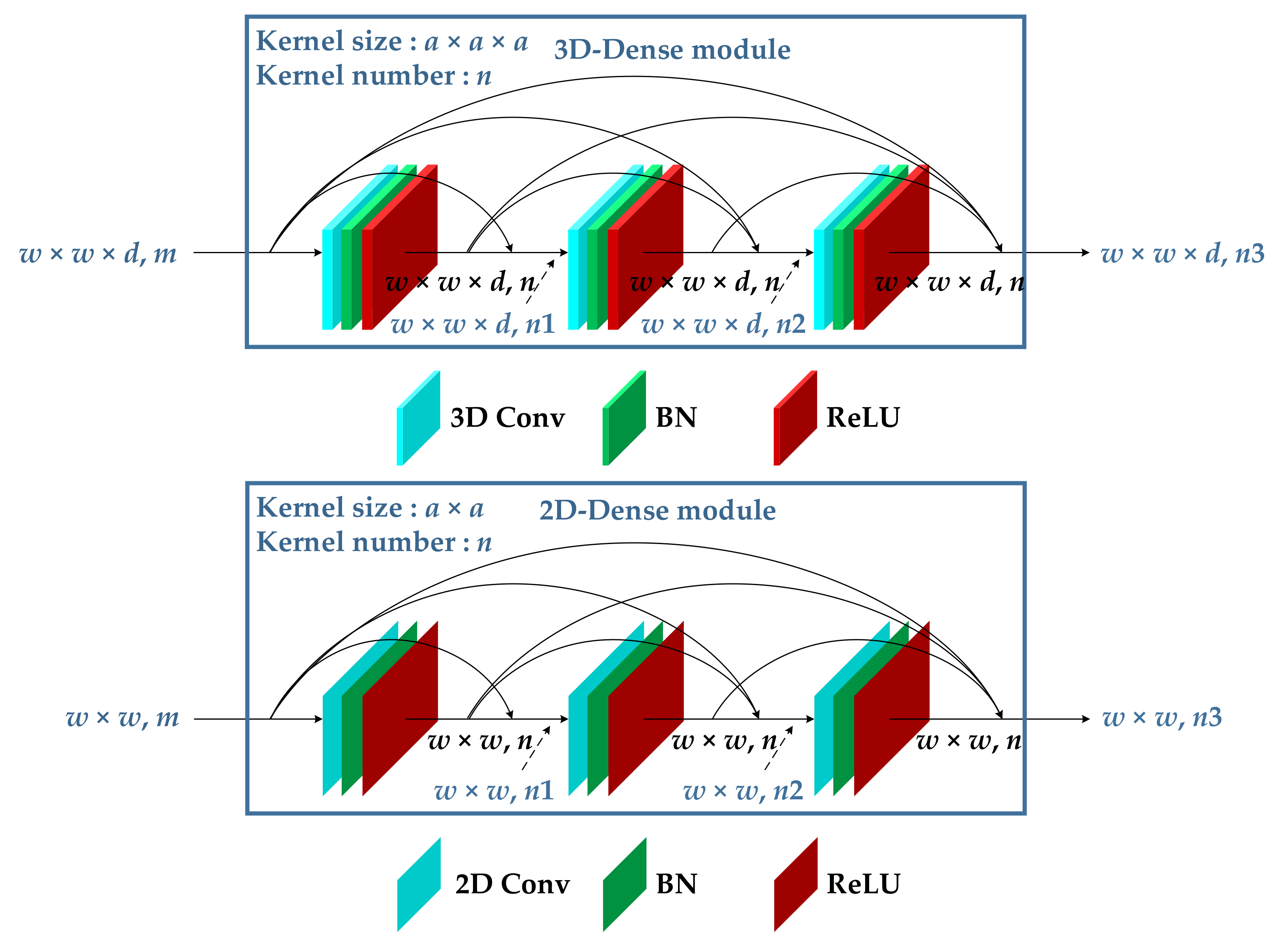
To make use of the attention mechanism and solve the problems of the SSRN and FDSSC, we proposed a hybrid dense network with dual attention (HDDA) for HSI classification. This framework contains two branches of 3D-DenseNet and 2D-DenseNet, which are used to extract spectral–spatial and spatial features, respectively, from dimension-reduced HSIs by the SAE. In addition, the residual channel attention and residual spatial attention are introduced for refining feature maps and avoiding unnecessary information. The enhanced spectral–spatial features are then obtained by connecting the outputs of two branches. Finally, classification results can be obtained using the softmax function. The main contributions of this work are listed as follows:

(1)

In order to deal with the nonlinear and high-dimensional problems of HSIs, a four-hidden-layer SAE network was built to effectively extract deep features and reduce the feature dimensions;

(2)

We proposed a hybrid dense network classifier with a dual-attention mechanism. The classification network has two independent feature-extraction paths, which continuously extract spectral–spatial features simultaneously in 3D and 2D spaces, respectively. The problem of feature conflict between the SSRN and FDSSC is avoided;

(3)

We constructed the residual dual-attention module. By integrating channel attention and spatial attention, the feature refinement was realized in the channel and spatial dimensions respectively. The results showed that spectral and spatial features had a better impact on the classification results, suppressing less useful features.

The rest of this study is arranged as follows: Three HSI datasets and evaluation factors for assessing the proposed network are described in Section 2. The background information is briefly introduced in Section 3. The proposed overall classification framework is presented in detail in Section 4. In Section 5, the experimental results are compared and discussed with reference to the ablation experiments. Finally, a summary and future directions are provided in Section 6.

2. Hyperspectral Datasets and Evaluation Factors

Three publicly available HSI datasets—namely, Indian Pines (IP), Pavia University (PU), and Salinas (SA)—were selected to verify the classification performance of the proposed HDDA method (

Table 1. Summary of three publicly available hyperspectral datasets: IP, PU, and SA *.

Dataset	Sensor	Wavelength Range (μm)	Pixel Size	Spatial Resolution (m)	Available Bands	Class Quantity
IP	Airborne visible/infrared imaging spectrometer (AVIRIS)	0.4~2.5	145 × 145	~20	200	16
PU	Reflective optics spectrographic imaging system (ROSIS-03)	0.43~0.86	610 × 340	1.3	103	9
SA	AVIRIS	0.4~2.5	512 × 217	3.7	204	16

* Denotes the data source: www.ehu.eus/ccwintco/index.php?title=Hyperspectral_Remote_Sensing_Scenes (accessed on 10 August 2021).

). The false-color composite images and ground-truth classes are shown in Figure 1, Figure 2 and Figure 3 and

Table 2. Number of training and test samples for the IP dataset.

Label	Class	Total	Training Set	Test Set
1	Alfalfa	46	2	44
2	Corn-notill	1428	71	1357
3	Corn-mintill	830	42	789
4	Corn	237	12	225
5	Grass-pasture	483	24	459
6	Grass-trees	730	37	694
7	Grass-pasture-mowed	28	1	27
8	Hay-windrowed	478	24	454
9	Oats	20	1	19
10	Soybean-notill	972	49	923
11	Soybean-mintill	2455	123	2332
12	Soybean-clean	593	30	563
13	Wheat	205	10	195
14	Woods	1265	63	1202
15	Buildings-Grass-Trees-Drives	386	19	367
16	Stone-Steel-Towers	93	5	88

,

Table 3. Number of training and test samples for the PU dataset.

Label	Class	Total	Training Set	Test Set
1	Asphalt	6631	66	6565
2	Meadows	18,649	186	18,463
3	Gravel	2099	21	2078
4	Trees	3064	31	3033
5	Painted metal sheets	1345	13	1332
6	Bare soil	5029	50	4979
7	Bitumen	1330	13	1317
8	Self-blocking bricks	3682	37	3645
9	Shadows	947	9	938

and

Table 4. Number of training and test samples for the SA dataset.

Label	Class	Total	Training Set	Test Set
1	Alfalfa	2009	20	1989
2	Corn-notill	3726	37	3689
3	Corn-mintill	1976	20	1956
4	Corn	1394	14	1380
5	Grass-pasture	2678	27	2651
6	Grass-trees	3959	40	3919
7	Grass-pasture-mowed	3579	36	3543
8	Hay-windrowed	11,271	113	11,158
9	Oats	6203	62	6141
10	Soybean-notill	3278	33	3245
11	Soybean-mintill	1068	11	1057
12	Soybean-clean	1927	19	1908
13	Wheat	916	9	907
14	Woods	1070	11	1059
15	Buildings-Grass-Trees-Drives	7268	73	7195
16	Stone-Steel-Towers	1807	18	1789

. For a general deep network, the more training samples, the better the classification performance. Unfortunately, it is usually time-consuming and laborious to collect enough label information from HSI data. It can be difficult or even impossible to provide sufficient training samples for most networks. Moreover, with the increase in the number of samples, the computational complexity and time consumption also increase correspondingly. Consequently, it is better to perform the classification using a small number of training samples. In our study, only 5%, 1%, and 1% of the samples from IP, UP, and SA, respectively, were selected as the training set, while the remaining samples were used to validate the classification performance.

The primary configuration of the computer included an Intel Corei5-7300HQ CPU (2.50 GHz), a GTX1050Ti GPU, and 8 GB RAM, with the Windows 10 64-bit operating system. The compiler was Spyder and the DL framework was PyTorch. To comparatively analyze the classification performance, the overall accuracy (OA), average accuracy (AA), and kappa coefficient (k) based on the confusion matrix were used as the evaluation factors [41]. OA is the ratio between the correctly classified samples and total samples. AA is the ratio between the sum of the classification accuracy for each category and the number of categories. k is generally used for checking consistency, and can be also used to measure the classification accuracy. The higher the three factors are, the better the classification performance.

3. Background Information

3.1. Stacked Autoencoder

An autoencoder (AE) is an unsupervised learning method, whose structure is similar to that of a general feedforward neural network; its function is to perform representation learning on the input information, which has been applied to dimension reduction and abnormal data detection [42,43]. In comparison with supervised learning methods, only the target data rather than labeled data are required to be input for the AE. In our study, a stacked AE (SAE) was built by stacking the basic autoencoders to extract the features from original HSIs and perform dimension reduction. An SAE is formed by stacking the basic AE network structure layer by layer according to the input layer and hidden layers (Figure 4).

The encoder is composed of one input layer and four hidden layers, and the decoder includes four hidden layers and one output layer. To ensure the same range of [0, 1] for the input layer and the output layer, the tanh nonlinear activation function is used for both the encoder and the decoder, while the sigmoid nonlinear activation function is adopted for the output layer. The mean squared error (MSE) loss function is used to measure the deviation between real and reconstructed data. The adaptive moment estimation (Adam) optimization algorithm is used to train the network parameters. With the increase in the number of layers, the features become more and more abstract. Meanwhile, the dimensions of the input data are continuously reduced, and the high-dimensional input data are transformed into low-dimensional features to reduce the original HSI data.

3.2. ResNet and DenseNet

With the increase in the number of network layers, the CNN model is prone to gradient disappearance during the training process. Conversely, the ResNet and DenseNet can solve the problem via skip connection and dense connection, respectively. As an essential part of ResNet, the residual connection is commonly used in ResNet, enabling the input data to be passed directly over the network to subsequent layers [44]. As a special form of ResNet, DenseNet, by connecting all of the layers directly, ensures the maximum information flow between the layers of the network [45]. Unlike the combined features obtained by summation for ResNet, the dense module is used to combine features by connecting them in the channel direction. The 3D- (Figure 5a) and 2D-Dense (Figure 5b) modules are jointly used to establish a hybrid dense network consisting of three convolutional layers (l = 3), where the ReLU activation function is adopted. The dense connection is used for each layer to connect the front and back layers, in order to build a deeper network structure.

3.3. Dual-Attention Mechanism

The basic idea of attention mechanisms in computer vision is to enable the network to ignore irrelevant information among numerous features and pay attention to the important features related to the current task [46,47]. Attention mechanisms can be divided into soft attention mechanisms and hard attention mechanisms. Hard attention mechanisms are non-differentiable, and need to be trained through strategies such as enhanced learning, while soft attention mechanisms are differentiable, wherein the network parameters can be updated during the training process by the gradient descent algorithm [48]. Therefore, the dual-attention mechanism combining channel attention and spatial attention was adopted in our study in order to strengthen the features with a large contribution to classification and suppress the features with only a small contribution (Figure 6).

3.3.1. Channel Attention Module

For the feature maps obtained by the CNN, different channels represent different types of features. The channel attention module reassigns the weight of channel dimensions according to the importance of different channels [49]. The detailed structure of the channel attention module is shown in Figure 6a. The feature map generated by the 3D convolutional layer is taken as an example. It is assumed that the input feature map is $F\in R^{w\times w\times c\times n^{\prime }}$, where w × w is the size, c is the spectral dimension, and n′ is the number of channels. Firstly, the 3D global average pooling and 3D global max pooling are each carried out on the whole input feature map F. Two different feature descriptors of $F_{avg}^c$ and $F_{max}^c$ are generated, and their dimensions are 1 × 1 × n′. The two descriptors are then input into the shared network (SN) consisting of a two-layer convolutional layer and an activation function layer, in order to generate feature maps with the dimensions of 1 × 1 × n′. Afterwards, the summation is used to merge the output feature vectors, and the channel attention map CA (F) is obtained via the sigmoid activation function. The channel attention map is a vector whose length is the same as the number of channels in the input feature map; its values are located within the range of (0, 1). The calculation process of channel attention is mathematically expressed as follows:

$$\begin{array}{cc}\hfill CA\left(F\right)& =\delta \left(SN\left(AvgPool\left(F\right)\right)+SN\left(MaxPool\left(F\right)\right)\right)\hfill \\ & =\delta \left(W_1{\delta }^{\prime }\left(W_0\left(F_{avg}^c\right)\right)+W_1{\delta }^{\prime }\left(W_0\left(F_{max}^c\right)\right)\right)\hfill \end{array}$$

(1)

where δ and δ′ represent the sigmoid and ReLU activation functions, respectively, and W₀ and W₁ are the weights of SN. Finally, the output feature map $F^{\prime }\in R^{w\times w\times c\times n^{\prime }}$ is obtained as shown in Equation (2):

$$F^{\prime }=CA\left(F\right)\otimes F$$

(2)

where CA (F) represents the channel attention map and F is the original input feature.

3.3.2. Spatial Attention Module

In comparison with channel attention, spatial attention focuses on the significant regions of the spatial dimension, which can further capture the contextual information of different regions [50,51]. The detailed structure of the spatial attention module is shown in Figure 6b. Similar to the channel attention module, two types of pooling operations are used to generate two feature descriptors of $F_{avg}^s$ and $F_{max}^s$, but the pooling operation is performed along the channel direction. Both of the two feature descriptors have the same dimensions of w × w × 1. Then, the joint operation results in an output feature descriptor of $\left[F_{avg}^s;F_{max}^s\right]$. A 3D convolutional layer with a sigmoid function is then used to generate a spatial attention map SA (F). The calculation process of channel attention is mathematically expressed as follows:

$$\begin{array}{cc}SA\left(F\right)& =\delta \left(f^{N\times N\times N}\left(\left[AvgPool\left(F\right);MaxPool\left(F\right)\right]\right)\right)\hfill \\ & =\delta \left(f^{N\times N\times N}\left[F_{avg}^s;F_{max}^s\right]\right)\hfill \end{array}$$

(3)

where δ represents the sigmoid activation function, while f^N×N×N represents the 3D convolution operation with a convolution kernel of N × N × N. The output feature map $F^{″}\in R^{w\times w\times c\times n^{\prime }}$ is obtained as shown in Equation (4):

$$F^{″}=SA\left(F\right)\otimes F$$

(4)

where SA (F) represents the spatial attention map and F is the original input feature.

3.3.3. Residual Dual-Attention Module

When the dual-channel attention module does not work, the original characteristic information of the entire network should not be reduced. The skip connection is introduced by referring to the ResNet. The high-level features revised by the channel attention and spatial attention are connected with the residual features to form the residual dual-attention module. The final output features of F_RDA are as shown in Equation (5). Through the residual connection structure, the information transfer in the model can be promoted; the gradient descent is alleviated and the stability of the model is enhanced. In addition, based on the hybrid CNN, the structures of the residual dual-attention module are slightly different for different input feature maps. More details can be found in Section 3.1.

$$F_{RDA}=\left[\left(F+F^{\prime }\right);\left(F+F^{″}\right)\right]$$

(5)

4. Methodology

4.1. Overall Workflow

To take advantage of 3D HSI data, we proposed a hybrid dense network framework with dual attention (HDDA) for HSI classification (Figure 7). Firstly, the dimensions of the original HSI data were reduced by the SAE, and then the center pixels with the neighborhood size of w × w and corresponding class labels were taken as the samples and randomly divided into training sets of X_train and Y_train and test sets of X_test and Y_test. Secondly, we constructed two independent feature-extraction paths. The residual dual-attention module was used to refine features, and then the training set was input into the HDDA network to be trained for obtaining the best network model. Finally, the test set was used to evaluate the performance of the trained model. As shown in Figure 7, two branches including 3D-Dense and 2D-Dense networks were jointly used to construct the feature-extraction network by introducing the dual-attention mechanism.

4.2. Hybrid Dense Network

The spatial–spectral features and spatially enhanced features of the HSI data were obtained by using the 3D-DenseNet and 2D-DenseNet with dual attention (Figure 8). Then, the fusion features obtained by merging the two networks were used to perform the classification. In our study, the addition operation was used to merge features through the full connection layer, and the dropout was used to prevent overfitting. Finally, the classification was carried out by the softmax. The IP dataset was taken as an example to describe the specific methodology.

4.2.1. 3D-DenseNet with Dual Attention

The 3D-DenseNet is composed of a 3D-Dense module and a 3D residual dual-attention module (Figure 8a and

Table 5. Details of the 3D-DenseNet with dual attention.

Layer Name	Kernel Size	Output	Number of Parameters
Input layer	-	(23 × 23 × 10, 1)	0
Conv3D	(3 × 3 × 3)	(23 × 23 × 10, 32)	896
Conv3D-BN-ReLU	(3 × 3 × 3)	(23 × 23 × 10, 16)	13,840
Concatenation	-	(23 × 23 × 10, 48)	0
Conv3D-BN-ReLU	(3 × 3 × 3)	(23 × 23 × 10, 16)	20,752
Concatenation	-	(23 × 23 × 10, 64)	0
Conv3D-BN-ReLU	(3 × 3 × 3)	(23 × 23 × 10, 16)	27,664
Concatenation	-	(23 × 23 × 10, 80)	0
Conv3D-BN-ReLU	(1 × 1 × 10)	(23 × 23 × 1, 80)	64,080
3D-Attention module	-	(23 × 23 × 1, 160)	25,975
BN-ReLU-Global Average Pooling	-	(1 × 160)	0

). The sample size of the input layer was set as 23 × 23 × 10 for the HDDA network. At first, a 3D convolution with a kernel size of 3 × 3 × 3 was used to increase the number of channels to 32. Then, the spatial–spectral features were extracted through the 3D-Dense module. There were 16 channels for each 3D convolution with the 3 × 3 × 3 convolution kernels. The size of the output feature map was (23 × 23 × 10, 80) through the dense module. To refine the spatial–spectral features, the 3D residual dual-attention mechanism was introduced to strengthen the space and channels that make a significant contribution to the classification. The joint dual-attention feature map can be generated with a size of (23 × 23 × 1, 160). Finally, the batch normalization (BN) layer was used to enhance the stability of the model, and a feature map of 1 × 160 was obtained through the global average pooling.

4.2.2. 2D-DenseNet with Dual Attention

In order to enhance the spatial information, the HSI cube with a sample size of 23 × 23 × 10 was reshaped and input into the 2D-DenseNet with dual attention, composed of a 2D-Dense module and a 2D residual dual-attention module (Figure 8b and

Table 6. Details of the 2D-DenseNet with dual attention.

Layer Name	Kernel Size	Output	Number of Parameters
Input Layer	-	(23 × 23, 10)	0
Conv2D	(3 × 3)	(23 × 23, 32)	2912
Conv2D-BN-ReLU	(3 × 3)	(23 × 23, 16)	4624
Concatenate	-	(23 × 23, 48)	0
Conv2D-BN-ReLU	(3 × 3)	(23 × 23, 16)	6928
Concatenate	-	(23 × 23, 64)	0
Conv2D-BN-ReLU	(3 × 3)	(23 × 23, 16)	9232
Concatenate	-	(23 × 23, 80)	0
Conv2D-BN-ReLU	(1 × 1)	(23 × 23, 80)	6480
2D-Attention module	-	(23 × 23, 160)	25,975
BN-ReLU-Global Average Pooling	-	(1 × 160)	0

). Firstly, the 2D convolution with a kernel size of 3 × 3 was adopted to increase the number of channels to 32 in order to obtain the feature map with dimensions of (23 × 23, 32). Then, the feature map was transferred into the 2D-Dense module. Three-layer 2D convolution with a convolution kernel size of 3 × 3 for each layer was produced. The size of the output feature map was (23 × 23, 80) through the 2D-Dense module. Subsequently, it was input into the 2D residual dual-attention module in order to obtain a dual-attention feature map with dimensions of (23 × 23, 160). Furthermore, the important spatial regions and channels were highlighted. After obtaining the dual-attention feature map, the BN layer and activation function were used to acquire a 1 × 160 feature map through global average pooling.

5. Results and Discussion

5.1. Configuration of Network Parameters

A hybrid dense network classification framework with a dual-attention mechanism was designed. The weight parameters of the SAE and dual-attention hybrid dense network were updated through the gradient backpropagation. This section focuses on analyzing several determinant factors affecting the classification effect of the HDDA, specifically including the window size (w) of the input sample, learning rate (lr), and dropout ratio (p). A total of 5%, 1%, and 1% of samples were randomly selected from each class of the IP, UP, and SA datasets, respectively, in order to train the model, while the remaining samples were used to verify the model. In addition, the reduced-dimension value (d) was set to 10, and the mean squared error (MSE) loss function and Adam optimization algorithm were used to train the HDDA. The batch size was set to 64 with 200 iterations, and the average value of 10 experiments was employed as the classification accuracy.

5.1.1. Window Size

The w affects the classification performance of a CNN to a great extent [52]. If the w value is small, the receptive field of feature extraction in the convolution kernel will be insufficient, and the local effect will not be good. A larger window size provides more spatial information, but more noises are also introduced, reducing the training speed. The short-term memory occupation increases, imposing higher requirements on the hardware platform. Consequently, an appropriate w can not only improve the training speed, but also improve the classification performance. To find the appropriate w for the three datasets, six window sizes were adopted (Figure 9). When the w of IP and SA is 15, and for PU is 19, their OA is the best.

5.1.2. Learning Rate

The lr plays an extremely important role in the classification performance for a DL-based network model [53]; it affects the training convergence speed of the model. If it is too small, the optimization efficiency may be too low to converge. When it is too large, the parameter adjustment changes quickly, and optimal values may be missing. Therefore, different lrs affect the classification performance for various datasets. Four lrs of 0.1, 0.01, 0.001, and 0.0001 were employed in order to compare the classification performance (Figure 10). It was found that, when the lr was 0.001, the HDDA had the best performance on the IP and SA datasets, with the highest OA values. Conversely, the HDDA performed best when the lr was 0.0001 for the PU dataset.

5.1.3. Dropout Ratio

Overfitting is one of the most common problems in neural network training, affecting the generalization performance of a model. Generally, the empirical error on the training samples is very small, while the generalization error on the test set is very large. Dropout is a regularization method in DL, which is beneficial to preventing overfitting and accelerates the training speed [54]. Five dropout ratios (ps) were set up to compare the classification performance for the three datasets (

Table 7. Comparison of OA with different dropout ratios for the three datasets.

p	OA
	IP	PU	SA
0.2	95.28	97.30	97.23
0.3	94.75	97.80	97.61
0.4	96.80	98.28	98.61
0.5	95.74	96.35	98.85
0.6	94.26	97.35	98.10

). When p was 0.4, HDDA had the best performance on the IP and PU datasets, with the highest OAs of 96.80% and 98.28%, respectively; when it was 0.5, the OA was highest for the SA dataset, reaching 98.85%. The accuracy and loss graphs for the three datasets also show similar results (Figure 11).

5.2. Experimental Results

To verify the effectiveness and robustness of the HDDA, the spectral-based REF-SVM [14] and four advanced HSI classification methods—3D-CNN [24], HybridSN [25], SSRN [30], and R-HybridSN [32]—were adopted. The parameter settings of the five comparative methods were consistent with those in the corresponding references.

5.2.1. IP Dataset

There are high similarities of different classes for the IP dataset, such as Corn (2–4), Grass (5–7) and Soybean (10–12). The sample size is small for certain classes, which makes it difficult to achieve a good classification performance. A total of 5% of the samples of the IP dataset were randomly selected as the training set, and the remainder were used as the test set. The classification results were derived from the mean and standard deviation (SD) of 10 experiments. A five-layer SAE structure was used to reduce the dimensions of the HSIs, and the number of nodes in each layer was set to 220-120-80-40-10. The reduced-dimension HSIs were then input into the HDDA, with a w of 15 × 15, a lr of 0.001, a p of 0.4, and an epoch of 200.

In comparison with the five other methods (

Table 8. Comparison of accuracy using the HDDA and five other methods for the IP dataset.

Label	Color	REF-SVM	3D-CNN	HybridSN	SSRN	R-HybridSN	HDDA
1		7.98	93.15	61.82	86.32	45.00	81.48
2		73.47	85.67	92.25	95.98	95.45	94.73
3		61.92	94.86	92.97	97.02	97.36	97.59
4		31.15	95.16	78.22	96.65	94.80	94.76
5		84.92	87.30	96.60	98.87	98.85	99.55
6		92.42	92.33	98.11	97.36	99.32	100.00
7		0.00	100.00	68.52	89.01	95.56	100.00
8		99.33	99.48	99.96	97.32	100.00	100.00
9		0.00	88.70	83.68	100.00	65.26	100.00
10		57.89	87.25	96.12	92.67	95.90	94.53
11		86.27	93.91	96.66	94.34	98.09	97.60
12		66.89	73.32	85.44	84.24	89.15	95.17
13		93.89	94.41	94.97	99.45	99.74	98.99
14		96.30	94.16	99.34	98.78	99.26	99.17
15		41.26	81.37	82.92	95.02	87.66	93.31
16		82.61	100.00	80.00	100.00	88.18	86.36
OA		77.66 ± 1.23	90.79 ± 0.31	94.24 ± 1.01	95.26 ± 0.18	96.46 ± 0.00	96.80 ± 0.10
AA		61.02 ± 1.37	91.32 ± 0.52	87.97 ± 1.93	95.19 ± 0.25	90.60 ± 0.33	95.83 ± 0.23
k		74.30 ± 0.72	89.68 ± 0.68	93.40 ± 0.01	94.55 ± 1.04	96.02 ± 1.53	96.34 ± 0.12

), the HDDA had the highest OA, AA, and k of 96.80%, 95.83%, and 96.34%, respectively. For those classes with fewer training samples, such as Grass-pasture-mowed (7) and Oats (9), their OA was not satisfactory when depending on the REF-SVM, which uses the spectral features to perform classification. Conversely, the other four DL-based classification methods—3D-CNN, HybridSN, SSRN, and R-HybridSN—showed advantages for processing small sample data, being able to extract the joint spatial–spectral features so as to achieve better classification. The OA of the two classes for the HDDA reached 100%. Due to the advantages of 3D convolution in extracting HSI cube data, the 3D-CNN can simultaneously extract spatial–spectral features, and its OA is improved by 13.13%. HybridSN improves the OA, AA, and k to 94.24%, 87.97%, and 93.40%, respectively, by combining a 3D-CNN and a 2D-CNN [25]. The HybridSN-based improved R-HybridSN introduces the residual module to deepen the network depth. A satisfactory classification performance can be obtained with an OA of 96.46% in the case of fewer training samples, which an improvement of 1.2% compared to the SSRN. In comparison with the SSRN, the OA, AA, and k of the HDDA were increased by 1.54%, 0.64%, and 1.79%, respectively, while they were increased by 0.34%, 5.23%, and 0.32%, respectively, compared with the R-HybridSN. In addition, the HDDA also achieved a good classification performance for those easily misclassified classes, such as the three kinds of Corn (2–4) and Soybeans (10–12), with OA of more than 94%. Consequently, there were fewer error points and better classification performance for the HDDA (Figure 12).

5.2.2. PU Dataset

Only 1% of the samples of the PU dataset were randomly selected as the training set, and the remainder were used as the test set. The number of nodes in each layer of the SAE was set to 103-80-60-40-10, and then the dataset was classified through the HDDA network. The w, lr, and p were set to 19 × 19, 0.0001, and 0.4, respectively, and a total of 200 epochs were recorded. The classification accuracy was obtained using the mean and SD of 10 experimental results.

As shown in

Table 9. Comparison of accuracy using the HDDA and five other methods for the PU dataset.

Label	Color	REF-SVM	3D-CNN	HybridSN	SSRN	R-HybridSN	HDDA
1		85.99	86.63	95.72	99.63	96.94	98.48
2		95.13	96.70	99.68	98.43	99.69	99.21
3		52.50	72.08	84.38	76.45	87.17	94.69
4		86.91	97.60	87.70	100.00	89.15	94.91
5		96.10	100.00	98.99	100.00	99.51	96.36
6		60.49	93.17	96.82	95.29	98.44	99.37
7		74.87	72.15	84.42	91.60	95.82	99.10
8		75.94	77.26	89.18	86.67	93.28	98.16
9		99.25	96.92	71.71	99.51	77.82	93.35
OA		84.80 ± 0.45	91.86 ± 0.36	95.09 ± 0.80	96.21 ± 0.22	96.59 ± 0.50	98.28 ± 0.01
AA		80.80 ± 0.60	88.06 ± 1.43	89.84 ± 1.93	94.18 ± 0.34	93.09 ± 1.20	97.07 ± 0.02
k		79.52 ± 0.98	89.14 ± 0.59	93.52 ± 0.01	94.69 ± 0.15	95.56 ± 0.00	97.72 ± 0.01

, the best classification performance was achieved by the HDDA, with OA, AA, and k of 98.28%, 97.07%, and 97.72%, respectively. Although the best classification could not be achieved for each class using our method, all of the classification accuracies were still more than 93%, indicating that it was able to capture distinguishing features among different classes. Due to the presence of sufficient samples for the UP dataset, the OA also reached 84.80% for the REF-SVM, but the accuracy was poor for the easily misclassified classes of Gravel (3) and Bitumen (7); conversely, the SSRN with a spatial–spectral residual model can extract deeper spatial–spectral features and, thus, increased the accuracy to 76.45% and 91.60%, respectively. In comparison with the SSRN, the R-HybridSN improved the accuracy of the two classes by 10.72% and 4.22%, respectively. Considering the performance of the HDDA, they were improved by 7.52% and 3.28%, respectively, compared with the R-HybridSN, while the OA, AA, and k increased by 1.69%, 3.98%, and 2.16% respectively. The classification map derived from the HDDA was smoother and more similar to the ground-truth map (Figure 13).

5.2.3. SA Dataset

Only 1% of the samples of each class were randomly selected as the training set, and the remainder were used as the test set. The number of nodes in each layer of the SAE was set to 224-120-80-40-10, and then input into the HDDA network for classification. The w, lr, and p were set to 15 × 15, 0.001, and 0.5, respectively, and the epochs were set to 200. The classification accuracy was also obtained based on the mean and SD of 10 experiments.

There are 16 classes and sufficient samples for each class of the SA dataset; it is relatively easy to distinguish various classes. As shown in

Table 10. Comparison of accuracy using the HDDA and five other methods for the SA dataset.

Label	Color	REF-SVM	3D-CNN	HybridSN	SSRN	R-HybridSN	HDDA
1		98.69	99.73	99.99	100.00	100.00	100.00
2		99.38	91.17	100.00	99.97	99.97	100.00
3		88.75	96.72	99.82	99.83	99.49	100.00
4		98.48	97.50	98.38	98.20	98.72	98.04
5		96.94	95.30	99.26	99.53	98.43	98.83
6		99.69	95.65	99.93	100.00	99.90	99.80
7		99.15	98.99	99.95	100.00	99.96	100.00
8		77.23	88.60	97.77	92.71	98.23	97.80
9		98.79	99.63	99.99	98.98	99.99	99.64
10		87.92	98.50	98.36	99.01	97.90	99.44
11		97.35	83.95	96.06	93.77	96.46	99.72
12		99.37	98.06	97.44	91.63	99.09	99.84
13		97.13	98.24	97.42	100.00	82.82	100.00
14		93.39	97.12	99.52	94.76	97.25	99.43
15		66.81	85.00	97.06	89.68	95.12	96.88
16		86.92	97.20	100.00	100.00	99.71	98.51
OA		88.47 ± 0.38	94.03 ± 0.17	98.72 ± 0.59	96.26 ± 0.12	98.25 ± 0.40	98.85 ± 0.01
AA		92.87 ± 0.42	95.09 ± 0.63	98.81 ± 0.50	97.38 ± 0.02	97.69 ± 0.69	99.25 ± 0.00
k		87.16 ± 0.78	93.14 ± 0.50	98.54 ± 0.00	96.02 ± 0.32	98.05 ± 0.00	98.72 ± 0.00

, the OA reached 88.47% for the RBF-SVM, but the classification accuracy of easily misclassified Vineyard_Untrained (15) was poor, at only 66.81%. It is easier to obtain a deeper knowledge of advanced features for the DL-based network models, which have more advantages to deal with the easily misclassified classes. The classification accuracy of Vineyard_Untrained was improved to 85% using the 3D-CNN—with OA, AA, and k values of 94.03%, 95.09%, and 93.14%, respectively—while it reached more than 97% for the HybridSN; in addition, compared with the SSRN and R-HybridSN, it was more competitive in terms of the classification performance for the SA dataset, with OA, AA, and k values of 98.72%, 98.81%, and 98.54%, respectively. By contrast, the classification accuracy of Vineyard_Untrained (15) for the HDDA was slightly lower than that of the HybridSN, but the OA, AA, and k were 0.13%, 0.44%, and 0.18% higher than for the HybridSN, respectively. Compared with the R-HybridSN, the OA, AA, and k were increased by 0.6%, 1.56% and 0.67%, respectively, indicating that the performance of the HDDA was the best. It is clear that there were fewer noise points on the classification map derived from the HDDA, with smoother visual effects (Figure 14).

5.3. Comparison of Training Percentages

In order to further verify the classification performance of the HDDA when using limited training samples, different proportions of the IP, PU, and SA datasets were set up. For the IP dataset, the proportions were 2%, 4%, 6%, 8%, and 10%, while for the UP and SA datasets, they were 0.2%, 0.4%, 0.6%, and 0.8%. The classification accuracy of the HDDA was comparatively analyzed by further reducing the number of training samples (Figure 15). It can be seen that the HDDA showed the best OA under different training proportions for all three datasets, reaching 88.57%, 86.93%, and 93.22% for the IP, PU, and SA datasets, respectively—even when using training percentages of 2% of IP, or 0.2% of PU and SA. Moreover, with the increase in the number of training samples, the HDDA showed better classification performance compared with the five other classification methods.

5.4. Ablation Experiments

In order to verify the effectiveness of the proposed hybrid network structure, SAE dimension-reduction method, and attention module, ablation experiments were conducted on the three hyperspectral datasets. The models used for comparison were consistent with the original network structure, except for the tested components.

5.4.1. Effectiveness of the Hybrid Dense Network

In this section, we performed the 3D branch and 2D branch without changing the other parameter settings. The OA was obtained based on the mean and SD of 10 experiments (

Table 11. Comparison of OA using three network structures for the three datasets.

Method	IP	PU	SA
2D branch	95.02 ± 1.40	95.37 ± 0.41	96.24 ± 0.26
3D branch	95.26 ± 0.12	97.01 ± 0.27	97.45 ± 0.07
HDDA (2D + 3D)	96.80 ± 0.10	98.28 ± 0.01	98.85 ± 0.01

). It was observed that the 3D branch is more suitable for processing HSIs than the 2D branch. In addition, because the HDDA method integrates the spatial–spectral features extracted by the 3D branch and the spatial features extracted by the 2D branch, it has higher and more stable classification accuracy.

5.4.2. Effectiveness of the SAE

In order to highlight the advantages of SAE dimensionality reduction, the PCA, locally linear embedding (LLE), and single-layer AE methods were used to reduce the dimensions of the original HSIs. The number of dimensions was set to 10, and the proposed HDDA network was used. As shown in Figure 16, in comparison with the three other methods, the OA for all three datasets was the highest when using the SAE. Specifically, the OA of the LLE method is slightly better than that of PCA, because LLE can deal with nonlinear problems to a certain extent. Conversely, the AE method performed the worst.

5.4.3. Effectiveness of the Dual-Attention Mechanism

To verify the effectiveness of the proposed dual-attention module, we conducted three experiments on the three datasets, i.e., without the attention mechanism (Model1), with only the spatial attention mechanism (Model2), and with only the channel attention mechanism (Model3). It is clear that the OA of the models using the attention mechanisms was higher than that of the model without the attention mechanisms, proving the effectiveness of the attention mechanisms (Figure 17). More specifically, the proposed HDDA method had the highest OA. Model2 performed better than Model3 on the IP and SA datasets, while Model3 performed better than Model2 on the PU dataset. This phenomenon shows that the spatial attention mechanism is superior to the channel attention mechanism for the three datasets.

6. Conclusions

Aiming at a limited sample size of HSI labeled data and the low classification accuracy of current neural network models, a hybrid dense network with a dual-attention mechanism was proposed from the perspective of network optimization. The network framework was established through a combination of two feature-extraction branches based on a 3D-CNN and a 2D-CNN. The use of dense modules deepened the network, reduced the problem of gradient disappearance, and extracted more robust spatial–spectral features. In addition, the dual-attention mechanism was introduced to the two feature-extraction branches, and corresponding weights were given in the spatial dimension and the channel dimension. The features in the HSIs were selectively learned, and different weights were assigned to corresponding features in order to further improve the feature-extraction capability of the network. Additionally, the BN layer and dropout layer were introduced, and the ReLU activation function was used to prevent the occurrence of overfitting and reduce the number of training parameters in order to achieve a faster convergence. Three publicly available hyperspectral datasets—IP, PU, and SA—were used to check the network. The results show that the HDDA has a superior classification performance compared with the five other methods. In the future, we will further study the attention mechanism and design more targeted attention modules in order to better solve the problem of small samples for HSIs.

References

1. He, L.; Li, J.; Liu, C.; Li, S. Recent advances on spectral-spatial hyperspectral image classification: An overview and new guidelines. IEEE Trans. Geosci. Remote Sens. 2018, 56, 1579–1597. [Google Scholar] [CrossRef]
2. Luo, F.; Du, B.; Zhang, L.; Zhang, L.; Tao, D. Feature learning using spatial-spectral hypergraph discriminant analysis for hyperspectral image. IEEE Trans. Cybern. 2019, 49, 2406–2419. [Google Scholar] [CrossRef]
3. Liu, B.; Yu, X.; Yu, A.; Wan, G. Deep convolutional recurrent neural network with transfer learning for hyperspectral image classification. J. Appl. Remote Sens. 2018, 12, 026028. [Google Scholar] [CrossRef]
4. Kumar, B.; Dikshit, O.; Gupta, A.; Singh, M.K. Feature extraction for hyperspectral image classification: A review. Int. J. Remote Sens. 2020, 41, 6248–6287. [Google Scholar] [CrossRef]
5. Zhang, H.; Li, Y.; Jiang, Y.; Wang, P.; Shen, Q.; Shen, C. Hyperspectral classification based on lightweight 3-D-CNN with transfer learning. IEEE Trans. Geosci. Remote Sens. 2019, 57, 5813–5828. [Google Scholar] [CrossRef] [Green Version]
6. Zhang, M.; Li, W.; Du, Q. Diverse region-based CNN for hyperspectral image classification. IEEE Trans. Image Process. 2018, 27, 2623–2634. [Google Scholar] [CrossRef]
7. Pan, B.; Shi, Z.; Xu, X. MugNet: Deep learning for hyperspectral image classification using limited samples. ISPRS J. Photogramm. Remote Sens. 2017, 145, 108–119. [Google Scholar] [CrossRef]
8. Fu, C.B.; Tian, A.H. Classification of hyperspectral images of small samples based on support vector machine and back propagation neural network. Sens. Mater. 2020, 32, 447–454. [Google Scholar] [CrossRef]
9. Abdi, H.; Williams, L.J. Principal component analysis. Wiley Interdiscip. Rev. Comput. Stat. 2010, 2, 433–459. [Google Scholar] [CrossRef]
10. Hou, Q.; Wang, Y.; Jing, L.; Chen, H. Linear discriminant analysis based on kernel-based possibilistic c-means for hyperspectral images. IEEE Geosci. Remote Sens. Lett. 2019, 16, 1259–1263. [Google Scholar] [CrossRef]
11. Jayaprakash, C.; Damodaran, B.B.; Viswanathan, S.; Soman, K.P. Randomized independent component analysis and linear discriminant analysis dimensionality reduction methods for hyperspectral image classification. J. Appl. Remote Sens. 2020, 14, 036507. [Google Scholar] [CrossRef]
12. Du, B.; Xiong, W.; Wu, J.; Zhang, L.; Zhang, L.; Tao, D. Stacked convolutional denoising auto-encoders for feature representation. IEEE Trans. Cybern. 2017, 47, 1017–1027. [Google Scholar] [CrossRef]
13. Khotimah, W.N.; Bennamoun, M.; Boussaid, F.; Sohel, F.; Edwards, D. A high-performance spectral-spatial residual network for hyperspectral image classification with small training data. Remote Sens. 2020, 12, 3137. [Google Scholar] [CrossRef]
14. Ji, Y.; Sun, L.; Li, Y.; Li, J.; Liu, S.; Xie, X.; Xu, Y. Non-destructive classification of defective potatoes based on hyperspectral imaging and support vector machine. Infrared Phys. Technol. 2019, 99, 71–79. [Google Scholar] [CrossRef]
15. Mario Haut, J.; Eugenia Paoletti, M.; Plaza, J.; Plaza, A. Fast dimensionality reduction and classification of hyperspectral images with extreme learning machines. J. Real-Time Image Process. 2018, 15, 439–462. [Google Scholar] [CrossRef]
16. Poona, N.K.; van Niekerk, A.; Nadel, R.L.; Ismail, R. Random Forest (RF) wrappers for waveband selection and classification of hyperspectral data. Appl. Spectrosc. 2016, 70, 322–333. [Google Scholar] [CrossRef] [PubMed]
17. Zhu, Z.; Wei, H.; Hu, G.; Li, Y.; Qi, G.; Mazur, N. A novel fast single image dehazing algorithm based on artificial multiexposure image fusion. IEEE Trans. Instrum. Meas. 2020, 70, 1–23. [Google Scholar] [CrossRef]
18. Han, Y.; Yin, M.; Duan, P.; Ghamisi, P. Edge-preserving filtering-based dehazing for remote sensing images. IEEE Geosci. Remote Sens. Lett. 2021, 1–5. [Google Scholar] [CrossRef]
19. Audebert, N.; Le Saux, B.; Lefevre, S. Deep learning for classification of hyperspectral data. IEEE Geosci. Remote Sens. Mag. 2019, 7, 159–173. [Google Scholar] [CrossRef] [Green Version]
20. Basha, S.H.S.; Dubey, S.R.; Pulabaigari, V.; Mukherjee, S. Impact of fully connected layers on performance of convolutional neural networks for image classification. Neurocomputing 2020, 378, 112–119. [Google Scholar] [CrossRef] [Green Version]
21. Yue, Q.; Ma, C. Hyperspectral data classification based on flexible momentum deep convolution neural network. Multimed. Tools Appl. 2018, 77, 4417–4429. [Google Scholar] [CrossRef]
22. Liu, Y.; Cao, G.; Sun, Q.; Siegel, M. Hyperspectral classification via deep networks and superpixel segmentation. Int. J. Remote Sens. 2015, 36, 3459–3482. [Google Scholar] [CrossRef]
23. Chen, Y.; Lin, Z.; Zhao, X.; Wang, G.; Gu, Y. Deep learning-based classification of hyperspectral data. IEEE J. Sel. Top. Appl. Earth Obs. Remote Sens. 2014, 7, 2094–2107. [Google Scholar] [CrossRef]
24. Chen, Y.; Zhao, X.; Jia, X. Spectral-spatial classification of hyperspectral data based on deep belief network. IEEE J. Sel. Top. Appl. Earth Obs. Remote Sens. 2015, 8, 2381–2392. [Google Scholar] [CrossRef]
25. Zhao, W.; Du, S. Spectral-spatial feature extraction for hyperspectral image classification: A dimension reduction and deep learning approach. IEEE Trans. Geosci. Remote Sens. 2016, 54, 4544–4554. [Google Scholar] [CrossRef]
26. Li, Y.; Zhang, H.; Shen, Q. Spectral–spatial classification of hyperspectral imagery with 3D convolutional neural network. Remote Sens. 2017, 9, 67. [Google Scholar] [CrossRef] [Green Version]
27. Roy, S.K.; Krishna, G.; Dubey, S.R.; Chaudhuri, B.B. HybridSN: Exploring 3-D-2-D CNN feature hierarchy for hyperspectral image classification. IEEE Geosci. Remote Sens. Lett. 2020, 17, 277–281. [Google Scholar] [CrossRef] [Green Version]
28. Kang, X.; Li, C.; Li, S.; Lin, H. Classification of hyperspectral images by Gabor filtering based deep network. IEEE J. Sel. Top. Appl. Earth Obs. Remote Sens. 2018, 11, 1166–1178. [Google Scholar] [CrossRef]
29. Chen, S.; Jin, M.; Ding, J. Hyperspectral remote sensing image classification based on dense residual three-dimensional convolutional neural network. Multimed. Tools Appl. 2021, 80, 1859–1882. [Google Scholar] [CrossRef]
30. Alotaibi, B.; Alotaibi, M. A hybrid deep ResNet and inception model for hyperspectral image classification. PFG J. Photogramm. Remote Sens. Geoinf. Sci. 2020, 88, 463–476. [Google Scholar] [CrossRef]
31. Li, G.; Zhang, C.; Lei, R.; Zhang, X.; Ye, Z.; Li, X. Hyperspectral remote sensing image classification using three-dimensional-squeeze-and-excitation-DenseNet (3D-SE-DenseNet). Remote Sens. Lett. 2020, 11, 195–203. [Google Scholar] [CrossRef]
32. Zhong, Z.; Li, J.; Luo, Z.; Chapman, M. Spectral-spatial residual network for hyperspectral image classification: A 3-D deep learning framework. IEEE Trans. Geosci. Remote Sens. 2018, 56, 847–858. [Google Scholar] [CrossRef]
33. Wang, W.; Dou, S.; Jiang, Z.; Sun, L. A fast dense spectral-spatial convolution network framework for hyperspectral images classification. Remote Sens. 2018, 10, 1068. [Google Scholar] [CrossRef] [Green Version]
34. Feng, F.; Wang, S.; Wang, C.; Zhang, J. Learning deep hierarchical spatial-spectral features for hyperspectral image classification based on residual 3D-2D CNN. Sensors 2019, 19, 5276. [Google Scholar] [CrossRef] [PubMed] [Green Version]
35. Liu, F.; Zheng, J.; Zheng, L.; Chen, C. Combining attention-based bidirectional gated recurrent neural network and two-dimensional convolutional neural network for document-level sentiment classification. Neurocomputing 2020, 371, 39–50. [Google Scholar] [CrossRef]
36. Haut, J.M.; Paoletti, M.E.; Plaza, J.; Plaza, A.; Li, J. Visual attention-driven hyperspectral image classification. IEEE Trans. Geosci. Remote Sens. 2019, 57, 8065–8080. [Google Scholar] [CrossRef]
37. Fang, B.; Li, Y.; Zhang, H.; Chan, J.C.-W. Hyperspectral images classification based on dense convolutional networks with spectral-wise attention mechanism. Remote Sens. 2019, 11, 159. [Google Scholar] [CrossRef] [Green Version]
38. Mei, X.; Pan, E.; Ma, Y.; Dai, X.; Huang, J.; Fan, F.; Du, Q.; Zheng, H.; Ma, J. Spectral-spatial attention networks for hyperspectral image classification. Remote Sens. 2019, 11, 963. [Google Scholar] [CrossRef] [Green Version]
39. Zhu, Z.; Luo, Y.; Qi, G.; Meng, J.; Li, Y.; Mazur, N. Remote sensing image defogging networks based on dual self-attention boost residual octave convolution. Remote Sens. 2021, 13, 3104. [Google Scholar] [CrossRef]
40. Sun, H.; Zheng, X.; Lu, X.; Wu, S. Spectral-spatial attention network for hyperspectral image classification. IEEE Trans. Geosci. Remote Sens. 2020, 58, 3232–3245. [Google Scholar] [CrossRef]
41. Lewis, H.G.; Brown, M. A generalized confusion matrix for assessing area estimates from remotely sensed data. Int. J. Remote Sens. 2001, 22, 3223–3235. [Google Scholar] [CrossRef]
42. Ghasrodashti, E.K.; Sharma, N. Hyperspectral image classification using an extended Auto-Encoder method. Signal Process. Image Commun. 2021, 92, 116111. [Google Scholar] [CrossRef]
43. Ramamurthy, M.; Robinson, Y.H.; Vimal, S.; Suresh, A. Auto encoder based dimensionality reduction and classification using convolutional neural networks for hyperspectral images. Microprocess. Microsyst. 2020, 79, 103280. [Google Scholar] [CrossRef]
44. He, K.; Zhang, X.; Ren, S.; Sun, J. Deep residual learning for image recognition. In Proceedings of the IEEE Conference on Computer Vision and Pattern Recognition, Las Vegas, NV, USA, 27–30 June 2016; pp. 770–778. Available online: https://doi.org/10.1109/CVPR.2016.90 (accessed on 10 September 2021).
45. Huang, G.; Liu, Z.; Weinberger, K.Q. Densely connected convolutional networks. In Proceedings of the IEEE Conference on Computer Vision and Pattern Recognition, Honolulu, HI, USA, 21–26 July 2017; pp. 2261–2269. Available online: https://doi.org/10.1109/CVPR.2017.243 (accessed on 9 October 2021).
46. Yang, J.; Sim, K.; Lu, W.; Jiang, B. Predicting stereoscopic image quality via stacked auto-encoders based on stereopsis formation. IEEE Trans. Multimed. 2019, 21, 1750–1761. [Google Scholar] [CrossRef]
47. Li, F.; Feng, R.; Han, W.; Wang, L. An augmentation attention mechanism for high-spatial-resolution remote sensing image scene classification. IEEE J. Sel. Top. Appl. Earth Obs. Remote Sens. 2020, 13, 3862–3878. [Google Scholar] [CrossRef]
48. Xu, R.; Tao, Y.; Lu, Z.; Zhong, Y. Attention-mechanism-containing neural networks for high-resolution remote sensing image classification. Remote Sens. 2018, 10, 1602. [Google Scholar] [CrossRef] [Green Version]
49. Zhao, X.; Zhang, J.; Tian, J.; Zhuo, L.; Zhang, J. Residual dense network based on channel-spatial attention for the scene classification of a high-resolution remote sensing image. Remote Sens. 2020, 12, 1887. [Google Scholar] [CrossRef]
50. Xu, Q.; Xiao, Y.; Wang, D.; Luo, B. CSA-MSO3DCNN: Multiscale octave 3D CNN with channel and spatial attention for hyperspectral image classification. Remote Sens. 2020, 12, 188. [Google Scholar] [CrossRef] [Green Version]
51. Xu, Y.; Zhang, L.; Du, B.; Zhang, F. Spectral-spatial unified networks for hyperspectral image classification. IEEE Trans. Geosci. Remote Sens. 2018, 56, 5893–5909. [Google Scholar] [CrossRef]
52. Zeng, H.; Edwards, M.D.; Liu, G.; Gifford, D.K. Convolutional neural network architectures for predicting DNA–protein binding. Bioinformatics 2016, 3, i121–i127. [Google Scholar] [CrossRef]
53. Wen, L.; Gao, L.; Li, X.; Zeng, B. Convolutional neural network with automatic learning rate scheduler for fault classification. IEEE Trans. Instrum. Meas. 2021, 70, 1–12. [Google Scholar] [CrossRef]
54. Garbin, C.; Zhu, X.; Marques, O. Dropout vs. batch normalization: An empirical study of their impact to deep learning. Multimed. Tools Appl. 2020, 79, 12777–12815. [Google Scholar] [CrossRef]
Figure 1. IP dataset: (a) false-color composite image; (b) ground-truth classes.
Remotesensing 13 04921 g001
Figure 2. PU dataset: (a) false-color composite image; (b) ground-truth classes.
Remotesensing 13 04921 g002
Figure 3. SA dataset: (a) false-color composite image; (b) ground-truth classes.
Remotesensing 13 04921 g003
Figure 4. Network structure of the proposed stacked autoencoder (SAE).
Remotesensing 13 04921 g004
Figure 5. Structures of the dense module used in our study (l = 3): (a) 3D-Dense module; (b) 2D-Dense module.
Remotesensing 13 04921 g005
Figure 6. Structure of the residual dual-attention module used in our framework: (a) channel attention module; (b) spatial attention module.
Remotesensing 13 04921 g006
Figure 7. The working procedure of our proposed HSI classification framework.
Remotesensing 13 04921 g007
Figure 8. Structure of the HDDA network: (a) 3D-DenseNet with dual attention; (b) 2D-DenseNet with dual attention.
Remotesensing 13 04921 g008
Figure 9. Comparison of OA using different w values for the three datasets.
Remotesensing 13 04921 g009
Figure 10. Comparison of OA using different lr values for the three datasets.
Remotesensing 13 04921 g010
Figure 11. Accuracy and loss graphs of the three datasets: (a) IP; (b) PU; (c) SA.
Remotesensing 13 04921 g011
Figure 12. Classification maps using only the training samples (5% of total samples) for the IP dataset. (a) False color image; (b) Ground truth; (c) REF-SVM; (d) 3D-CNN; (e) HybridSN; (f) SSRN; (g) R-HybridSN; (h) HDDA.
Remotesensing 13 04921 g012
Figure 13. Classification maps using only the training samples (1% of total samples) for the PU dataset. (a) False color image; (b) Ground truth; (c) REF-SVM; (d) 3D-CNN; (e) HybridSN; (f) SSRN; (g) R-HybridSN; (h) HDDA.
Remotesensing 13 04921 g013
Figure 14. Classification maps using only the training samples (1% of total samples) for the SA dataset. (a) False color image; (b) Ground truth; (c) REF-SVM; (d) 3D-CNN; (e) HybridSN; (f) SSRN; (g) R-HybridSN; (h) HDDA.
Remotesensing 13 04921 g014
Figure 15. Comparison of OA for six methods using different training percentages: (a) IP; (b) PU; (c) SA.
Remotesensing 13 04921 g015
Figure 16. Comparison of OA using four dimension-reduction methods for three datasets.
Remotesensing 13 04921 g016
Figure 17. Comparison of OA using four attention mechanisms for three datasets.
Remotesensing 13 04921 g017