
A Vehicle-Borne Mobile Mapping System Based Framework for Semantic Segmentation and Modeling on Overhead Catenary System Using Deep Learning


Abstract
:
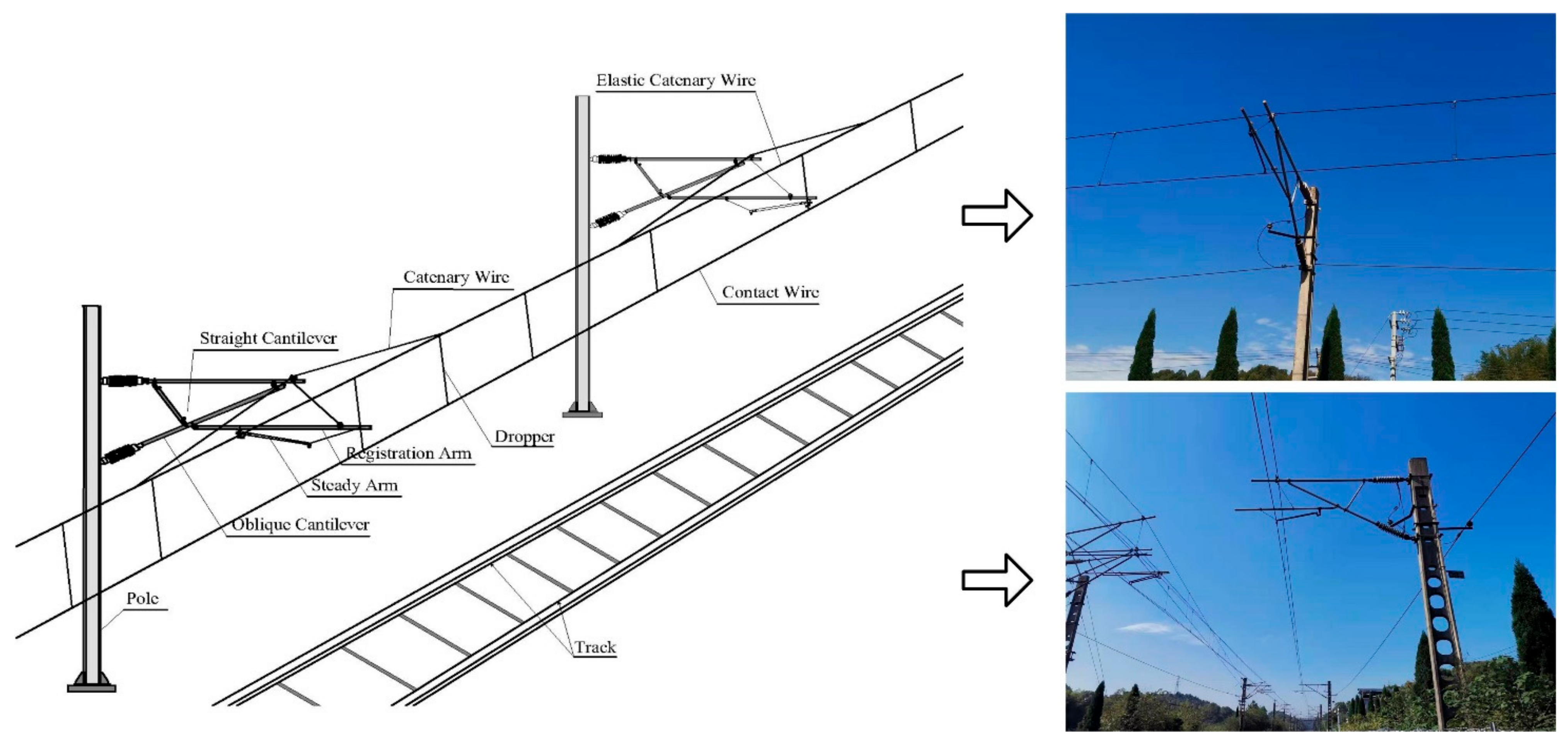
1. Introduction
2. Related Works
2.1. Statistics-Based Method
2.2. Deep-Learning-Based Method
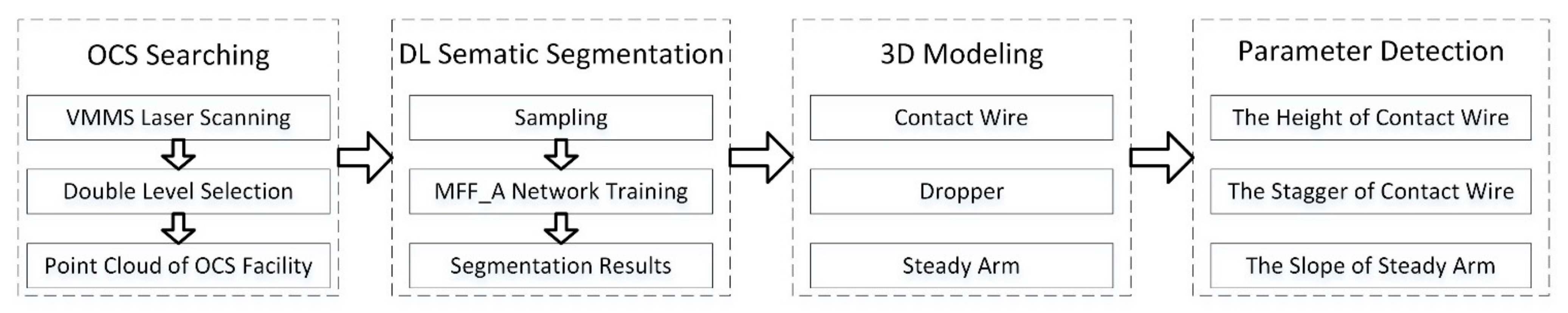
3. Material and Methodology
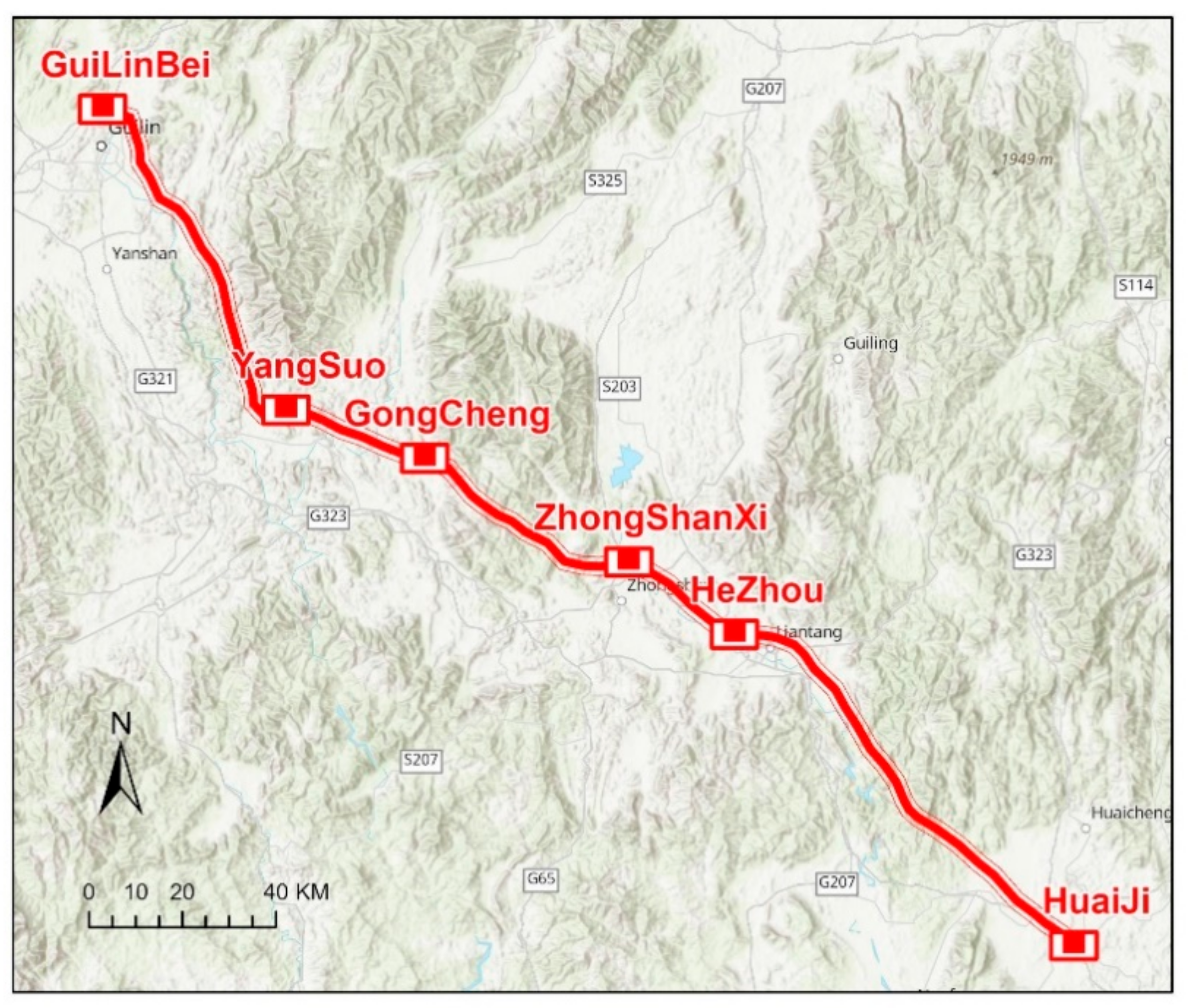
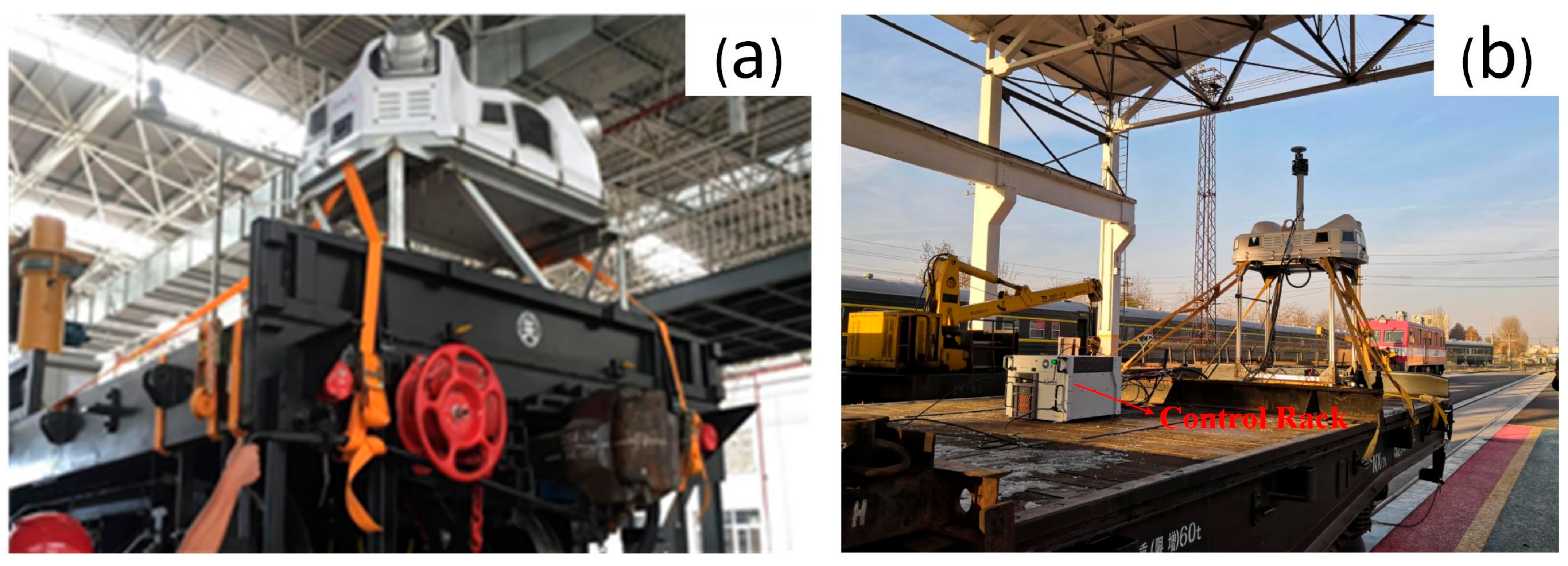
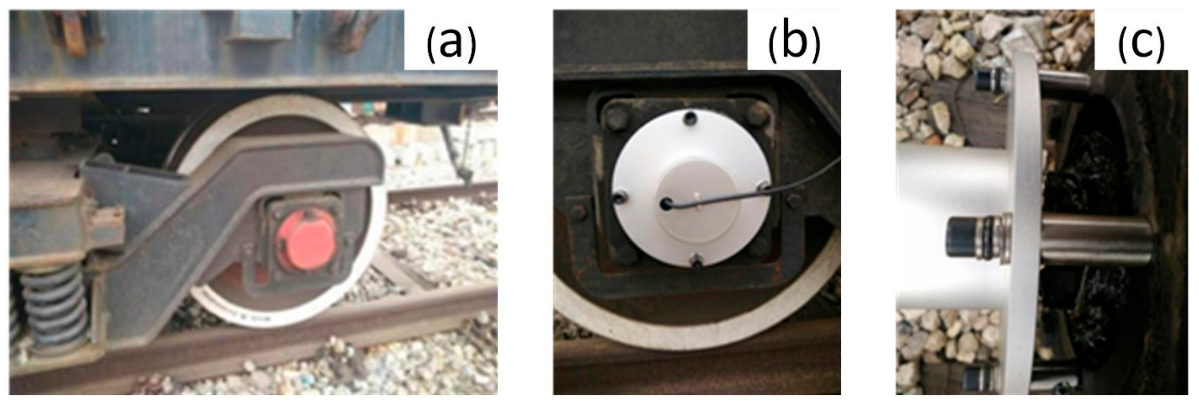
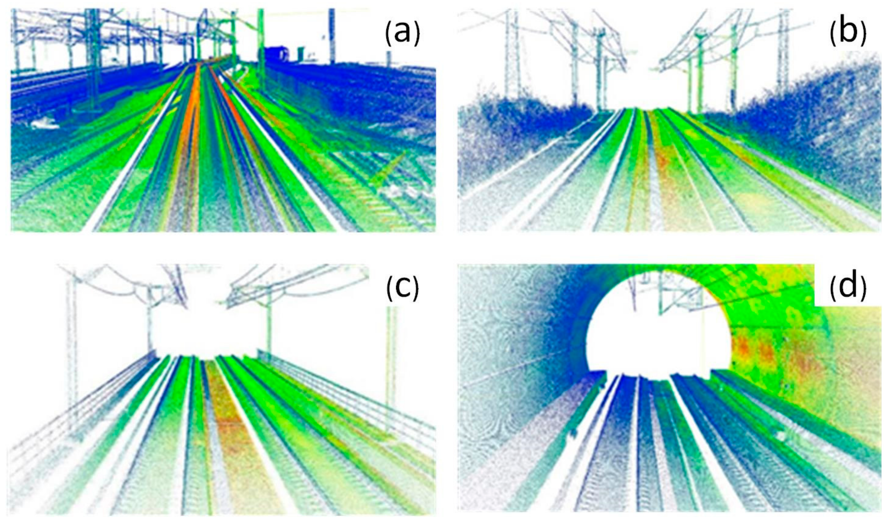
3.1. Study Area and VMMS Data Generation
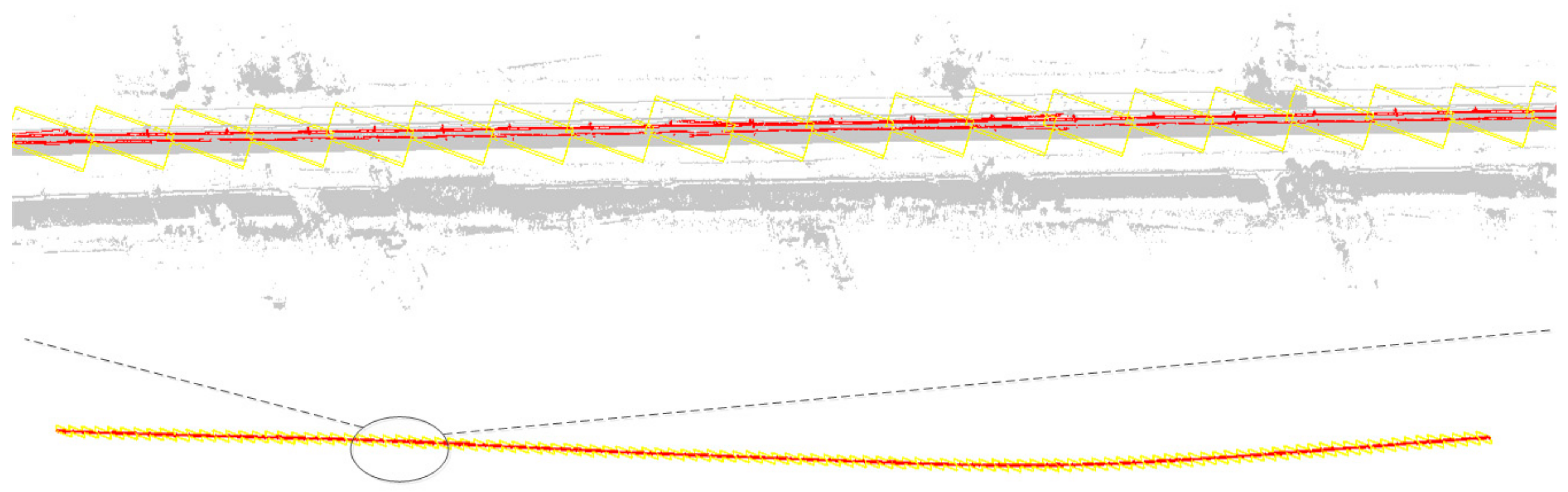
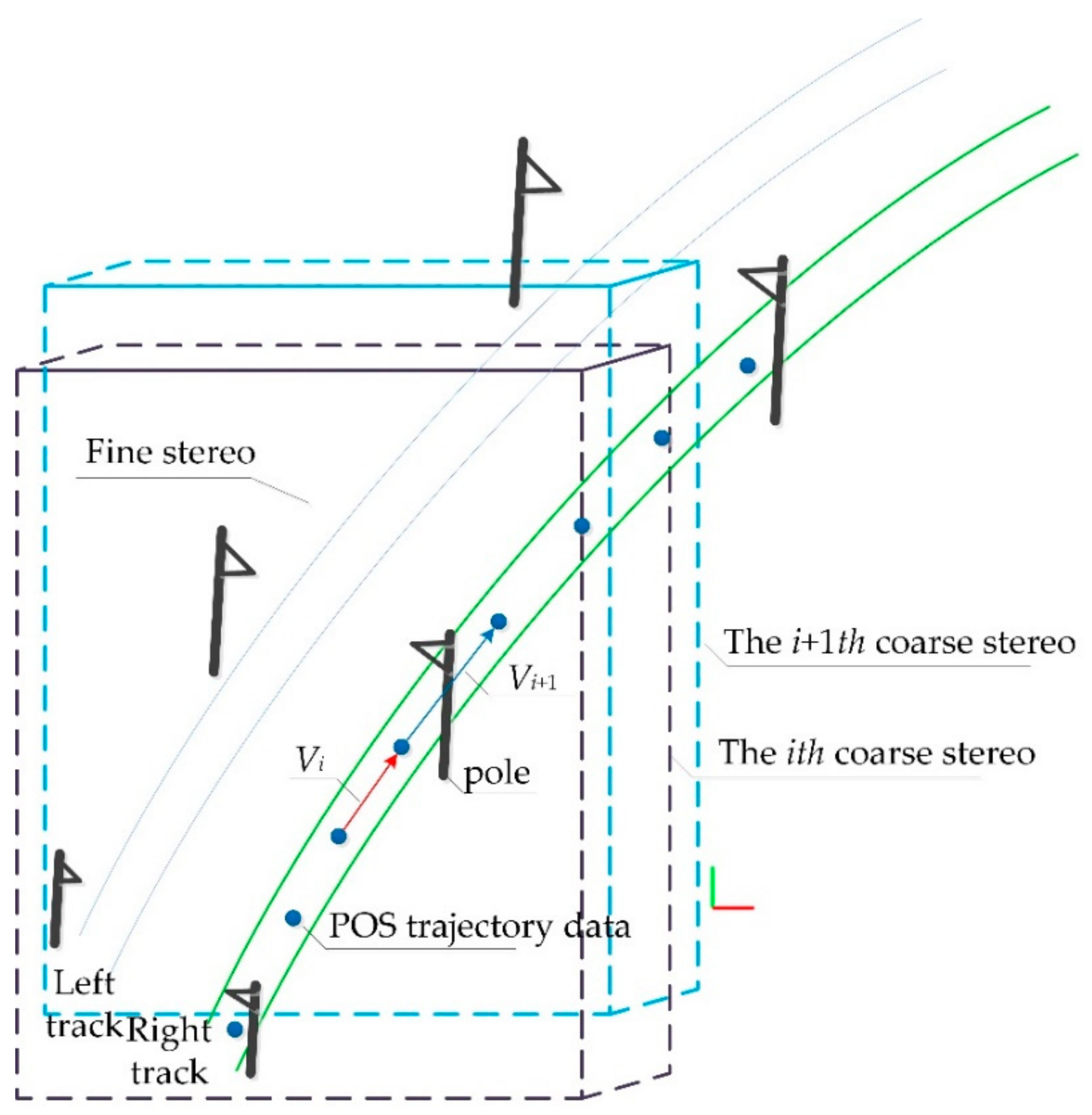
3.2. Double Selection Stereo Frame of OCS
| Algorithm 1. Automatic extraction algorithm of OCS facilities |
Input: Rail region point cloud: C = {Ck}, k = 1, 2, 3, …, M POS Trajectory lines L = {li}, I = 1, 2, 3, …, N An initial coarse selection of stereo frame
Output: Segmented and extracted rail region point cloud data CD = {CDj}, j = 1, 2, 3, …, H |
- Coarse selection of stereo frame posture and positioning
- Fine selection of stereo frame posture and positioning
- Determination of distance offset of dual selection stereo frame
- Track data-assisted posture auto-adjustment for selected stereo frame
- Clipping and extraction of contact network facilities
3.3. Deep Learning Based Semantic Segmentation
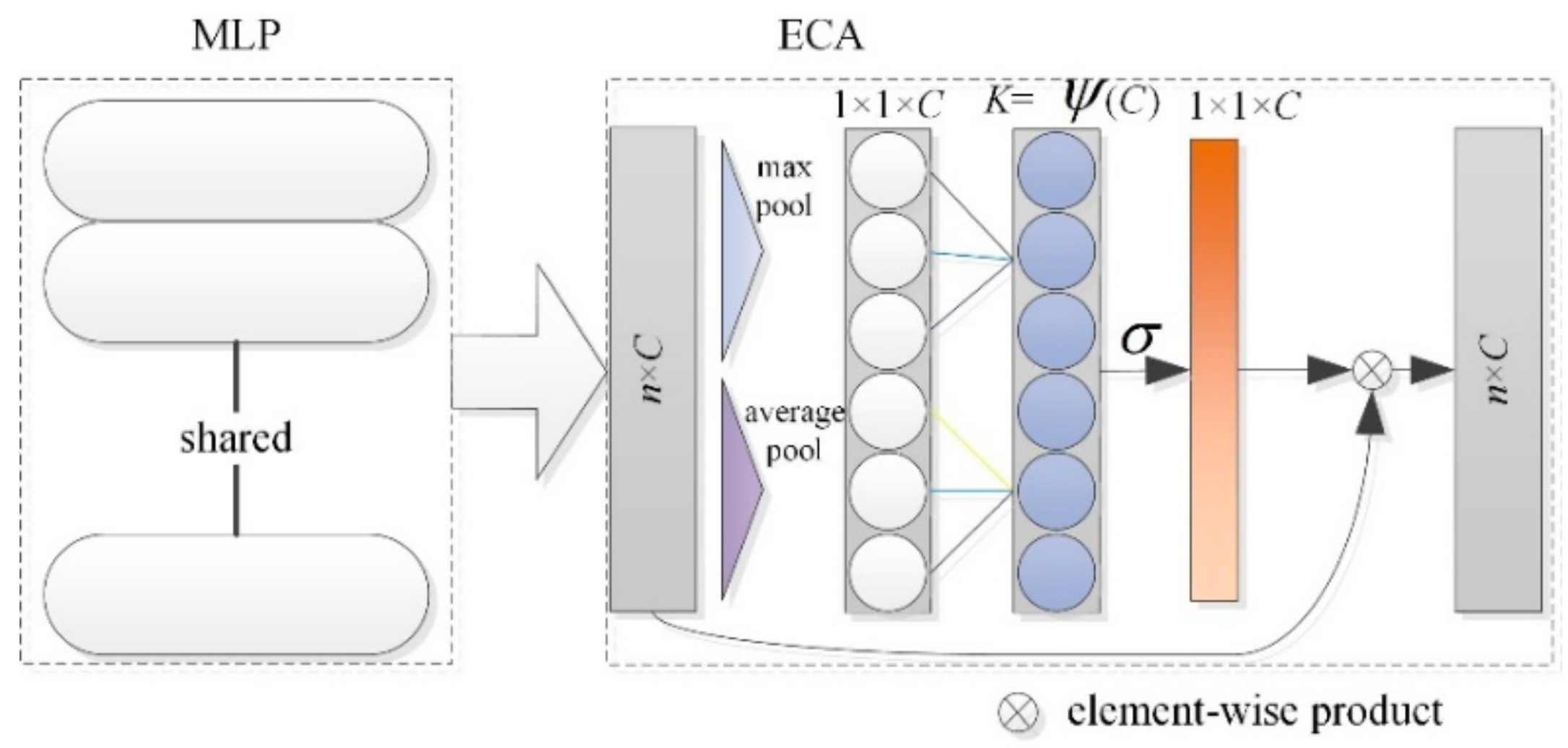
3.3.1. ECA
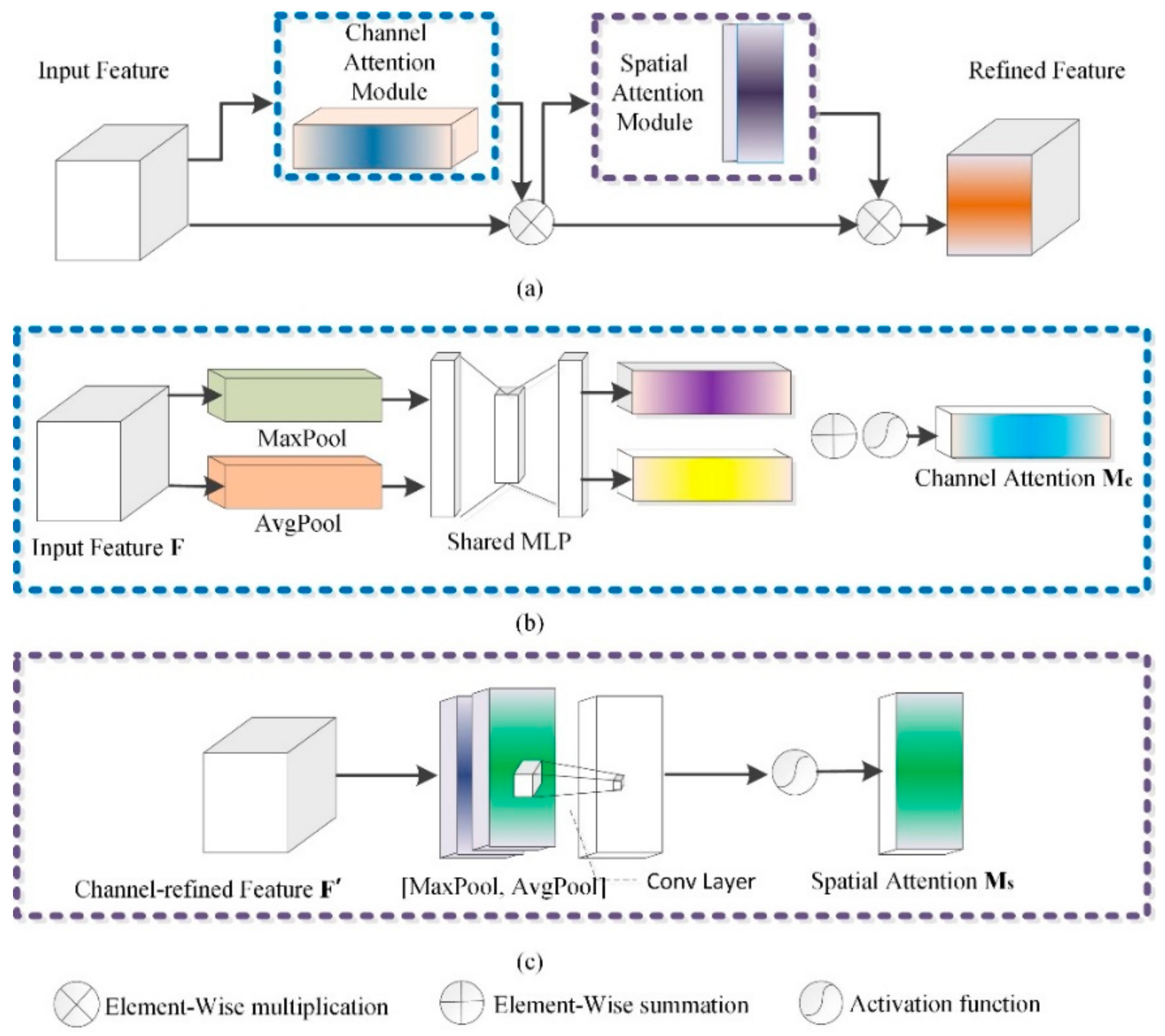
3.3.2. CBAM
- (1)
- Channel attention submodule in CBAM
- (2)
- Spatial attention submodule in CBAM
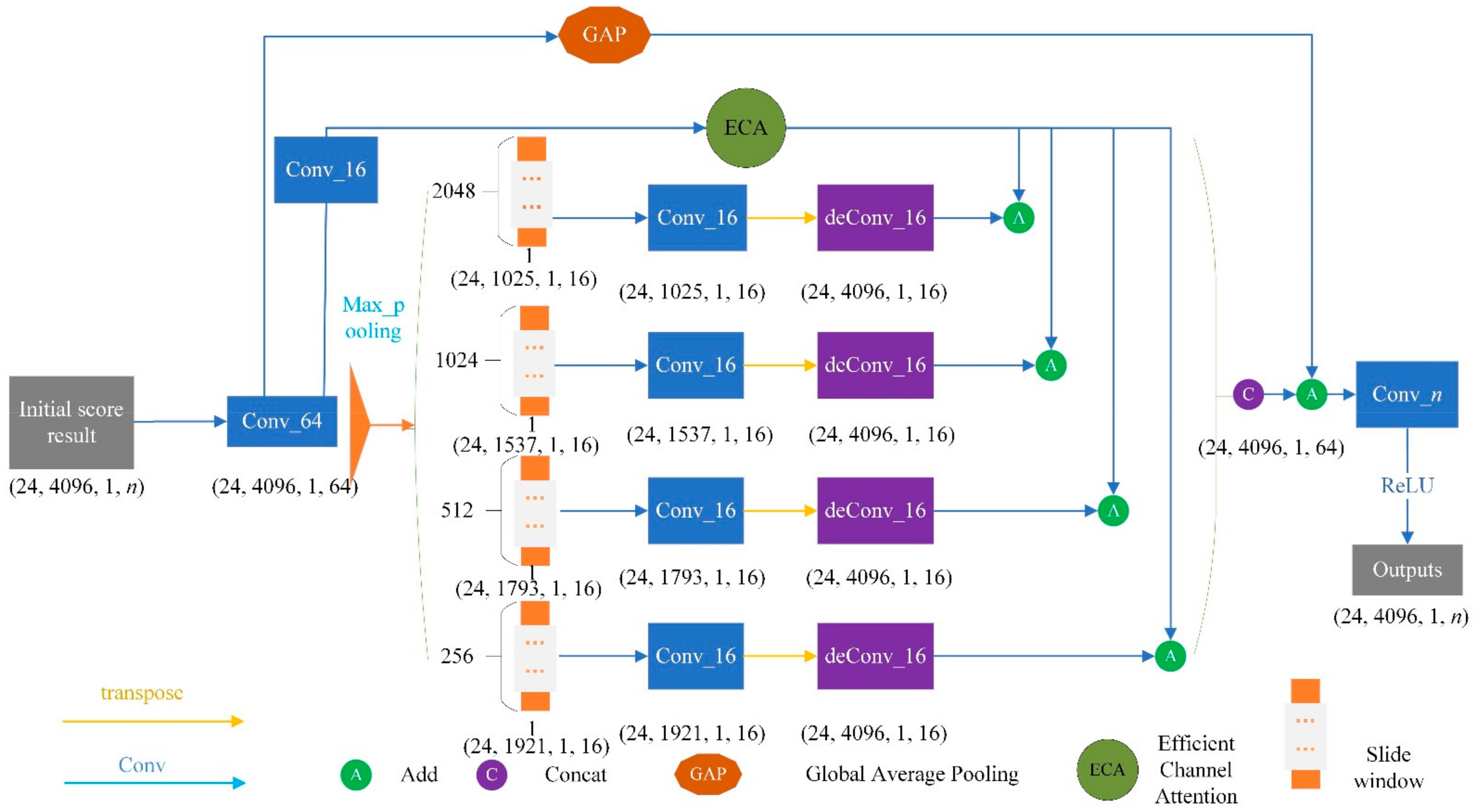
3.3.3. Refine Structure
3.3.4. Channel Feature Enhancement
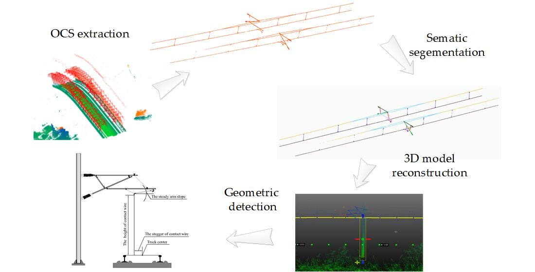
3.4. 3D Model Reconstruction and Parameter Detection of OCS
4. Results and Analysis
4.1. Search Result
4.2. MFF_A Segmentation
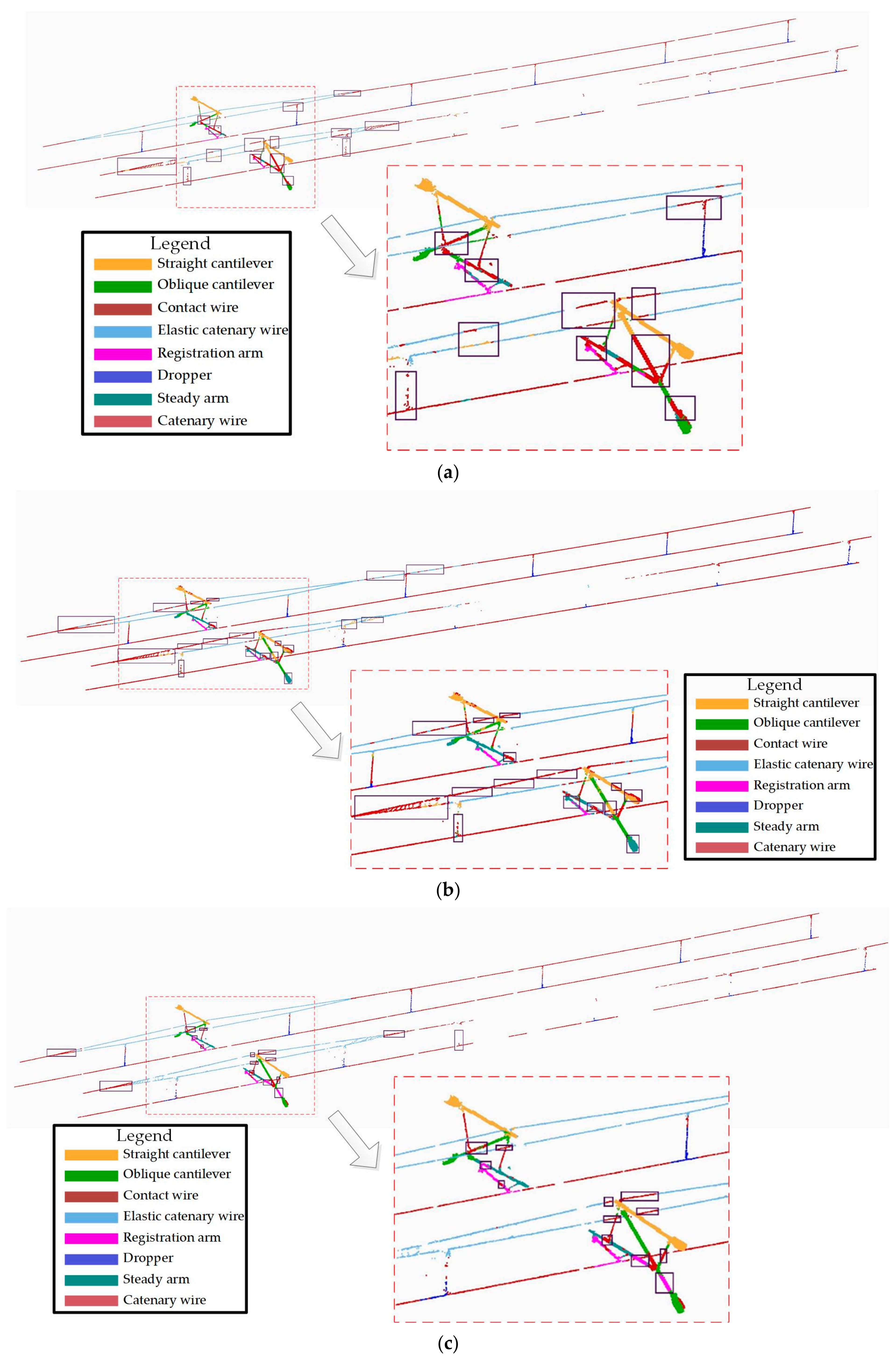
4.2.1. Segmentation Results
4.2.2. Quantitative Evaluation of the Segmentation Results
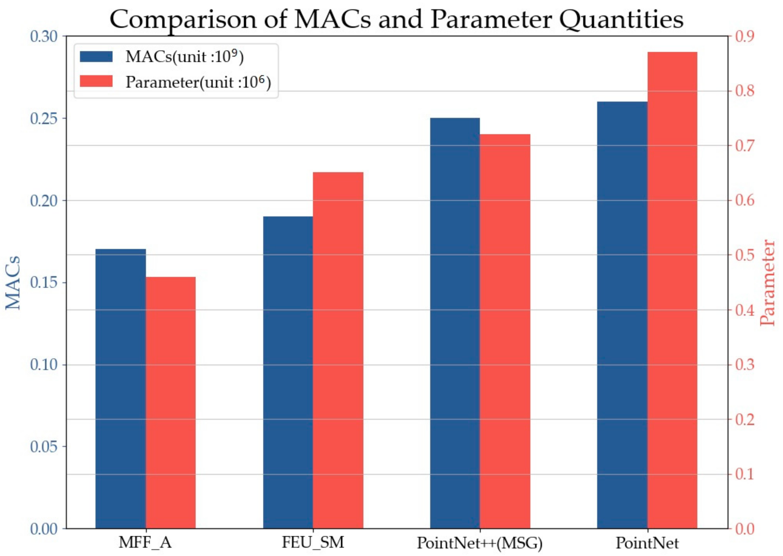
4.2.3. Parameter Complexity
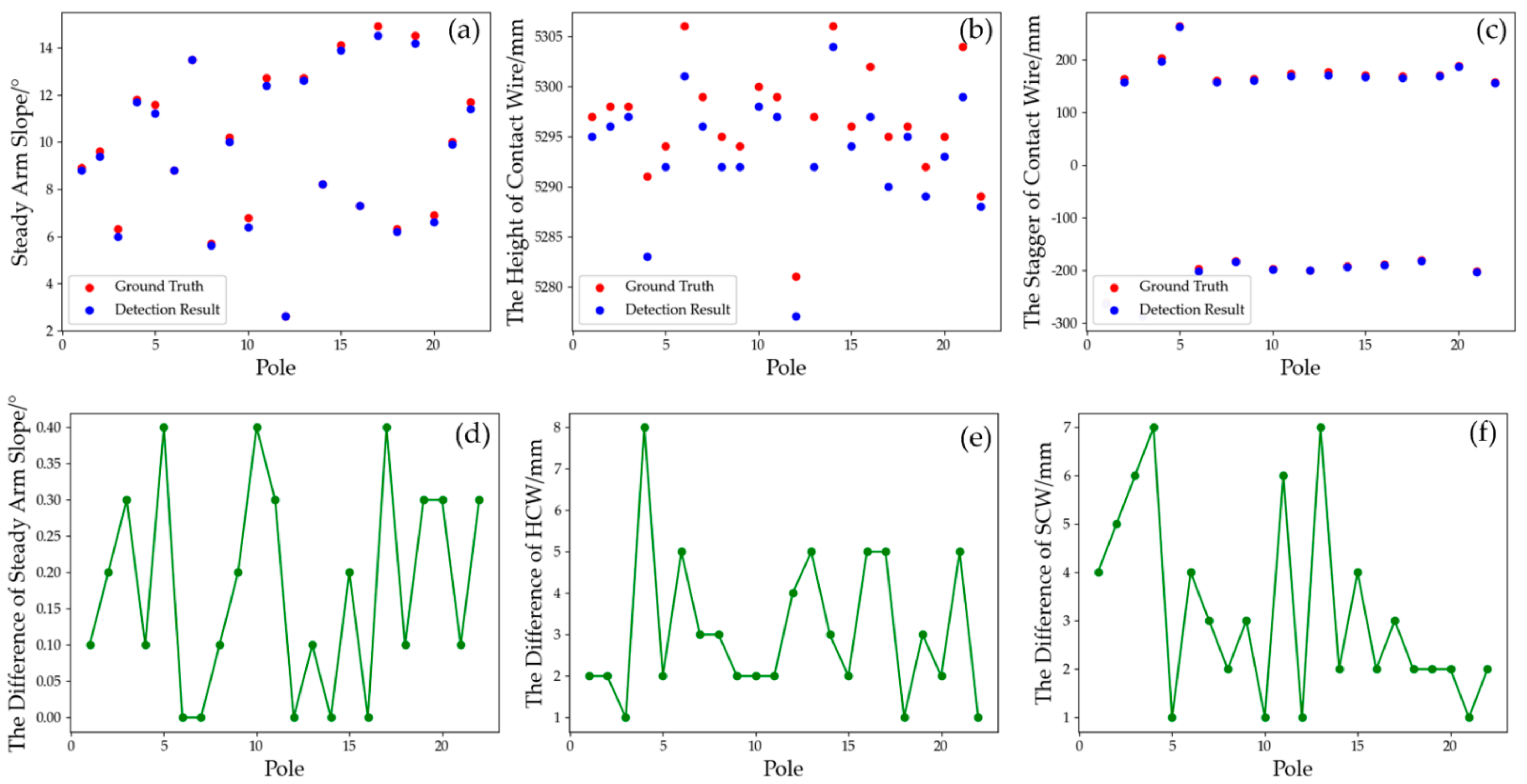
4.3. Geometric Evaluation of Reconstruction Results
5. Conclusions and Future Works
Author Contributions
Funding
Data Availability Statement
Acknowledgments
Conflicts of Interest
References
- Feng, X.; He, S.-W.; Li, Y.-B. Temporal characteristics and reliability analysis of railway transportation networks. Transp. A Transp. Sci. 2019, 15, 1825–1847. [Google Scholar] [CrossRef]
- Zhang, Q.; Liu, S.; Gong, D.; Zhang, H.; Tu, Q. An Improved multi-objective quantum-behaved particle swarm optimization for railway freight transportation routing design. IEEE Access 2019, 7, 157353–157362. [Google Scholar] [CrossRef]
- State Council Information Office of the People’s Republic of China. Sustainable Development of Transportation in China; People’s Publishing House: Beijing, China, 2020. [Google Scholar]
- Xiukun, W.; Da, S.; Dehua, W.; Xiaomeng, W.; Siyang, J.; Ziming, Y. A survey of the application of machine vision in rail transit system inspection. Control. Decis. 2021, 36, 257–282. [Google Scholar]
- Wanju, Y. High Speed Electrified Railway Catenary; Southwest Jiaotong University Press: Chengdu, China, 2003. [Google Scholar]
- Tan, P.; Li, X.; Wu, Z.; Ding, J.; Ma, J.; Chen, Y.; Fang, Y.; Ning, Y. Multialgorithm fusion image processing for high speed railway dropper failure–defect detection. IEEE Trans. Syst. Man Cybern. Syst. 2021, 51, 4466–4478. [Google Scholar] [CrossRef]
- Kang, G.; Gao, S.; Yu, L.; Zhang, D. Deep architecture for high-speed railway insulator surface defect detection: Denoising autoencoder with multitask learning. IEEE Trans. Instrum. Meas. 2019, 68, 2679–2690. [Google Scholar] [CrossRef]
- Lin, S.; Xu, C.; Chen, L.; Li, S.; Tu, X. LiDAR point cloud recognition of overhead catenary system with deep learning. Sensors 2020, 20, 2212. [Google Scholar] [CrossRef] [Green Version]
- Gutiérrez-Fernández, A.; Fernández-Llamas, C.; Matellán-Olivera, V.; Suárez-González, A. Automatic extraction of power cables location in railways using surface LiDAR systems. Sensors 2020, 20, 6222. [Google Scholar] [CrossRef]
- Zhong, J.; Liu, Z.; Han, Z.; Han, Y.; Zhang, W. A CNN-based defect inspection method for catenary split pins in high-speed railway. IEEE Trans. Instrum. Meas. 2019, 68, 2849–2860. [Google Scholar] [CrossRef]
- Han, Y.; Liu, Z.; Lyu, Y.; Liu, K.; Li, C.; Zhang, W. Deep learning-based visual ensemble method for high-speed railway catenary clevis fracture detection. Neurocomputing 2020, 396, 556–568. [Google Scholar] [CrossRef]
- Chen, L.; Xu, C.; Lin, S.; Li, S.; Tu, X. A deep learning-based method for overhead contact system component recognition using mobile 2D LiDAR. Sensors 2020, 20, 2224. [Google Scholar] [CrossRef] [Green Version]
- Dongxing, Z. Geometric parameter measurement of high-speed railroad OCS (Overhead Contact System) based on template matching image algorithm. Railw. Qual. Control. 2015, 43, 11–14. [Google Scholar]
- Liu, Y.; Han, T.; Liu, H. Study on OCS dynamic geometric parameters detection based on image processing. Railw. Locomot. Car 2012, 32, 86–91. [Google Scholar]
- Pastucha, E. Catenary system detection, localization and classification using mobile scanning data. Remote Sens. 2016, 8, 801. [Google Scholar] [CrossRef] [Green Version]
- Zou, R.; Fan, X.; Qian, C.; Ye, W.; Zhao, P.; Tang, J.; Liu, H. An efficient and accurate method for different configurations railway extraction based on mobile laser scanning. Remote Sens. 2019, 11, 2929. [Google Scholar] [CrossRef] [Green Version]
- Zhou, J.; Han, Z.; Wang, L. A steady arm slope detection method based on 3D point cloud segmentation. In Proceedings of the 2018 IEEE 3rd International Conference on Image, Vision and Computing (ICIVC), Chongqing, China, 27–29 June 2018; pp. 278–282. [Google Scholar]
- Lamas, D.; Soilán, M.; Grandío, J.; Riveiro, B. Automatic point cloud semantic segmentation of complex railway environments. Remote Sens. 2021, 13, 2332. [Google Scholar] [CrossRef]
- Jung, J.; Chen, L.; Sohn, G.; Luo, C.; Won, J.-U. Multi-range conditional random field for classifying railway electrification system objects using mobile laser scanning data. Remote Sens. 2016, 8, 1008. [Google Scholar] [CrossRef] [Green Version]
- Jingsong, Z.; Zhiwei, H.; Changjiang, Y. Catenary geometric parameters detection method based on 3D point cloud. Chin. J. Sci. Instrum. 2018, 39, 239–246. [Google Scholar]
- Chen, D.; Li, J.; Di, S.; Peethambaran, J.; Xiang, G.; Wan, L.; Li, X. Critical points extraction from building façades by analyzing gradient structure tensor. Remote Sens. 2021, 13, 3146. [Google Scholar] [CrossRef]
- Huang, R.; Xu, Y.; Stilla, U. GraNet: Global relation-aware attentional network for ALS point cloud classification. arXiv 2012, arXiv:13466 2020. [Google Scholar]
- Qi, C.R.; Su, H.; Mo, K.; Guibas, L.J. Pointnet: Deep learning on point sets for 3d classification and segmentation. In Proceedings of the IEEE Conference on Computer Vision and Pattern Recognition, Honolulu, HI, USA, 21–26 July 2017; pp. 652–660. [Google Scholar]
- Qi, C.R.; Yi, L.; Su, H.; Guibas, L.J. Pointnet++: Deep hierarchical feature learning on point sets in a metric space. arXiv 2017, arXiv:1706.02413. [Google Scholar]
- Li, Y.; Bu, R.; Sun, M.; Wu, W.; Di, X.; Chen, B. Pointcnn: Convolution on x-transformed points. Adv. Neural Inf. Process. Syst. 2018, 31, 820–830. [Google Scholar]
- Zhao, H.; Jiang, L.; Fu, C.-W.; Jia, J. PointWeb: Enhancing local neighborhood features for point cloud processing. In Proceedings of the 2019 IEEE/CVF Conference on Computer Vision and Pattern Recognition (CVPR), Long Beach, CA, USA, 15–20 June 2019; pp. 5560–5568. [Google Scholar]
- Thomas, H.; Qi, C.R.; Deschaud, J.-E.; Marcotegui, B.; Goulette, F.; Guibas, L. KPConv: Flexible and deformable convolution for point clouds. In Proceedings of the 2019 IEEE/CVF International Conference on Computer Vision (ICCV), Seoul, Korea, 27–28 October 2019; pp. 6411–6420. [Google Scholar]
- Wu, W.; Qi, Z.; Fuxin, L. PointConv: Deep convolutional networks on 3D point clouds. In Proceedings of the 2019 IEEE/CVF Conference on Computer Vision and Pattern Recognition (CVPR), Long Beach, CA, USA, 15–20 June 2019; pp. 9613–9622. [Google Scholar]
- Fu, J.; Liu, J.; Tian, H.; Li, Y.; Bao, Y.; Fang, Z.; Lu, H. Dual attention network for scene segmentation. In Proceedings of the IEEE/CVF Conference on Computer Vision and Pattern Recognition (CVPR), Long Beach, CA, USA, 15–20 June 2019; pp. 3141–3149. [Google Scholar]
- Hu, J.; Shen, L.; Sun, G. Squeeze-and-excitation networks. In Proceedings of the IEEE Conference on Computer Vision and Pattern Recognition (CVPR), Salt Lake City, UT, USA, 18–23 June 2018; pp. 7132–7141. [Google Scholar]
- Woo, S.; Park, J.; Lee, J.-Y.; Kweon, I.S. Cbam: Convolutional block attention module. In Proceedings of the European conference on computer vision (ECCV), Munich, Germany, 8–14 September 2018; pp. 3–19. [Google Scholar]
- Wang, Q.; Wu, B.; Zhu, P.; Li, P.; Zuo, W.; Hu, Q. ECA-Net: Efficient channel attention for deep convolutional neural networks. In Proceedings of the IEEE/CVF Conference on Computer Vision and Pattern Recognition (CVPR), Seattle, WA, USA, 14–19 June 2020; pp. 11531–11539. [Google Scholar] [CrossRef]
- Zhang, H.; Zu, K.; Lu, J.; Zou, Y.; Meng, D. Epsanet: An efficient pyramid split attention block on convolutional neural network. arXiv 2021, arXiv:2105.14447. [Google Scholar]
- Zhao, H.; Shi, J.; Qi, X.; Wang, X.; Jia, J. Pyramid scene parsing network. In Proceedings of the 2017 IEEE Conference on Computer Vision and Pattern Recognition (CVPR), Honolulu, HI, USA, 21–26 July 2017; pp. 6230–6245. [Google Scholar]
- Fang, H.; Lafarge, F. Pyramid scene parsing network in 3D: Improving semantic segmentation of point clouds with multi-scale contextual information. ISPRS J. Photogramm. Remote Sens. 2019, 154, 246–258. [Google Scholar] [CrossRef] [Green Version]
- Zhan, D.; Jing, D.; Wu, M.; Zhang, D. Study on dynamic vision measurement for locator slope gradient of electrified railway overhead catenary. J. Electron. Meas. Instrum. 2018, 32, 50–58. (In Chinese) [Google Scholar]
- TJ/GD006-2014. Provisional Technical Conditions for Catenary Suspension Condition Detection and Monitoring Device (4C); China Railway Publishing House Co., Ltd.: Beijing, China, 2014. [Google Scholar]


| OCS Type Classification | Proposed MFF_A | FEU_SM | PointNet++ (MSG) | PointNet | ||||
|---|---|---|---|---|---|---|---|---|
| P | IoU | P | IoU | P | IoU | P | IoU | |
| Steady arm | 96.34 | 86.21 | 95.69 | 87.60 | 90.38 | 85.31 | 92.46 | 81.65 |
| Straight cantilever | 93.64 | 88.63 | 90.65 | 87.46 | 91.86 | 85.76 | 86.49 | 78.91 |
| Oblique cantilever | 92.95 | 89.40 | 91.21 | 84.65 | 91.46 | 86.94 | 87.61 | 76.59 |
| Registration arm | 94.51 | 92.65 | 95.39 | 93.08 | 95.60 | 91.74 | 93.12 | 88.32 |
| Elastic catenary wire | 98.61 | 96.48 | 99.42 | 99.03 | 98.06 | 97.59 | 98.64 | 98.16 |
| Dropper | 95.65 | 92.32 | 96.44 | 91.36 | 95.25 | 93.17 | 90.78 | 75.49 |
| Contact wire | 99.87 | 99.69 | 99.39 | 99.14 | 99.68 | 98.33 | 99.28 | 98.75 |
| Catenary wire | 99.39 | 99.29 | 99.35 | 99.26 | 98.23 | 98.01 | 97.04 | 96.49 |
| Average | 96.37 | 93.08 | 95.94 | 92.70 | 95.07 | 92.11 | 93.18 | 86.80 |
Publisher’s Note: MDPI stays neutral with regard to jurisdictional claims in published maps and institutional affiliations. |
© 2021 by the authors. Licensee MDPI, Basel, Switzerland. This article is an open access article distributed under the terms and conditions of the Creative Commons Attribution (CC BY) license (https://creativecommons.org/licenses/by/4.0/).
Share and Cite
Xu, L.; Zheng, S.; Na, J.; Yang, Y.; Mu, C.; Shi, D. A Vehicle-Borne Mobile Mapping System Based Framework for Semantic Segmentation and Modeling on Overhead Catenary System Using Deep Learning. Remote Sens. 2021, 13, 4939. https://doi.org/10.3390/rs13234939
Xu L, Zheng S, Na J, Yang Y, Mu C, Shi D. A Vehicle-Borne Mobile Mapping System Based Framework for Semantic Segmentation and Modeling on Overhead Catenary System Using Deep Learning. Remote Sensing. 2021; 13(23):4939. https://doi.org/10.3390/rs13234939
Chicago/Turabian StyleXu, Lei, Shunyi Zheng, Jiaming Na, Yuanwei Yang, Chunlin Mu, and Debin Shi. 2021. "A Vehicle-Borne Mobile Mapping System Based Framework for Semantic Segmentation and Modeling on Overhead Catenary System Using Deep Learning" Remote Sensing 13, no. 23: 4939. https://doi.org/10.3390/rs13234939
APA StyleXu, L., Zheng, S., Na, J., Yang, Y., Mu, C., & Shi, D. (2021). A Vehicle-Borne Mobile Mapping System Based Framework for Semantic Segmentation and Modeling on Overhead Catenary System Using Deep Learning. Remote Sensing, 13(23), 4939. https://doi.org/10.3390/rs13234939