A Convolutional Neural Network Algorithm for Soil Moisture Prediction from Sentinel-1 SAR Images

Abstract

Achieving the rational, optimal, and sustainable use of resources (water and soil) is vital to drink and feed 9.725 billion by 2050. Agriculture is the first source of food production, the biggest consumer of freshwater, and the natural filter of air purification. Hence, smart agriculture is a “ray of hope” in regard to food, water, and environmental security. Satellites and artificial intelligence have the potential to help agriculture flourish. This research is an essential step towards achieving smart agriculture. Prediction of soil moisture is important for determining when to irrigate and how much water to apply, to avoid problems associated with over- and under-watering. This also contributes to an increase in the number of areas being cultivated and, hence, agricultural productivity and air purification. Soil moisture measurement techniques, in situ, are point measurements, tedious, time-consuming, expensive, and labor-intensive. Therefore, we aim to provide a new approach to detect moisture content in soil without actually being in contact with it. In this paper, we propose a convolutional neural network (CNN) architecture that can predict soil moisture content over agricultural areas from Sentinel-1 images. The dual-pol (VV–VH) Sentinel-1 SAR data have being utilized (V = vertical, H = horizontal). The CNN model is composed of six convolutional layers, one max-pooling layer, one flatten layer, and one fully connected layer. The total number of Sentinel-1 images used for running CNN is 17,325 images. The best values of the performance metrics (coefficient of determination ($R^2=0.8664$), mean absolute error ($MAE=0.0144$), and root mean square error ($RMSE=0.0274$)) have been achieved due to the use of Sigma naught VH and Sigma naught VV as input data to the CNN architecture (C). Results show that VV polarization is better than VH polarization for soil moisture retrieval, and that Sigma naught, Gamma naught, and Beta naught have the same influence on soil moisture estimation.

1. Introduction

Water is the “mainspring” that determines the survival and development of life on Earth. Arable land continues to be lost due to urbanization and desertification [1]. The world population is projected to reach 9.725 billion by 2050 [2]. Accordingly, work should be done to increase agricultural production and improve water management, to absorb population growth and its requirements for food and water.

Soil moisture content is generally defined as the temporary storage of water within the upper layer of soil [3]. Knowledge of soil water content plays a pivotal role in improving efficient water management [4]. Irrigation scheduling is an important water management strategy, which refers to the perfect amount of irrigation to apply to the field and the perfect timing for application [5]. Irrigation scheduling depends on the estimate of the soil moisture content [6]. The measurement of soil moisture content in situ is hard and expensive because it necessitates a repeated sampling process to analyze the periodical changes in soil moisture [7]. All soil moisture content measurement methods are divided into two broad categories—direct and indirect monitoring [8]. The most common techniques used for estimating soil moisture content in situ are gravimetric, neutron probe, time domain reflectometry (TDR), frequency domain reflectometry (FDR), and tensiometer techniques [9].

Research in the retrieval of soil moisture from satellite imagery has been vital in the past three decades, and we expect this trend to continue into the following decades. Surface soil moisture (SSM) is the water content available in the upper 0–5 cm of the soil layer, whereas the water that is available to plants is called root zone soil moisture, which is generally considered to be in the upper 0–200 cm of soil layer [9]. Therefore, estimating the amount of soil moisture in the root zone is more valuable and effective than surface soil moisture in agricultural and hydrological applications [10]. Direct determination of soil moisture in the root zone by remote sensing satellites is a laborious task and a serious challenge [11]. Direct soil observations are only possible in the case of bare soil (i.e., absence of vegetation) and, therefore, detecting soil moisture using remote sensing is suitable for a few days per year [12]. Compared to the visible and infrared, microwaves have many special qualities and advantages that are important for remote sensing [13]. Microwaves have long wavelengths—radiations can penetrate cloud cover, haze, and dust [14]. This characteristic enables detection of microwave energy in all environmental and weather conditions; hence, the ability to collect and capture data anytime [15]. Microwave remote sensing methods are suited for the detection and determination of soil moisture in the upper centimeters of the soil [16]. Synthetic aperture radar (SAR) satellite imaging is a promising method for soil moisture monitoring [17]. SAR systems can be used to investigate and retrieve soil moisture (0–5 cm depth) over agricultural areas [18]. The Sentinel-1 (S1) satellite characteristics include high spatial resolution and high revisit time; hence, Sentinel-1 is suitable for mapping and monitoring soil moisture over agricultural areas [19]. Sentinel-1 images can be used to retrieve soil moisture over wheat-covered areas [20]. VV polarization was more sensitive for soil moisture retrieval from Sentinel-1 data as compared to VH polarization [21,22,23]. Several studies have indicated that the accuracy of the soil moisture estimates improved when using both VV and VH polarization, instead of only VV or VH polarization [24,25,26].

Artificial intelligence is an integrated environment of various scientific fields [27]. Artificial intelligence is the simulation of human intelligence in machines [28]. Machine learning is one of the most important branches of artificial intelligence [29]. Machine learning aims to develop algorithms that are capable of learning, improving, and generalizing from a given collection of examples [30] without being explicitly programmed [31]. Deep learning is a specialized subset of machine learning [32]. In deep learning, a convolutional neural network (CNN) is a special class of artificial neural networks [33]. CNN is famous for its accurate and computationally efficient, powerful learning ability, and automatic high-level feature extraction [34]. CNN is one of the best available techniques for unstructured data types [35]. CNN has showed impressive achievements across a wide variety of domains, especially in computer vision related fields [36]. CNN is most commonly applied to analyze images [37], and feature extraction from images [38]. CNN can achieve a better performance than the linear regression model [39], and the support vector regression [40].

From the above, we conclude that all soil moisture measurement methods under field conditions are accurate with varying degrees. Common challenges and problems that exist in soil moisture measurement methods under field conditions are (1) point measurement methods (meaning, these techniques can only express soil moisture at specific points, and not at the entire cultivated area). (2) Regular periodic maintenance, thus require intensive labor. (3) The need for site-specific calibration. (4) The actual contact with the soil; and (5) the costs. We, therefore, intend to provide a new approach to knowing moisture content in soil without actually being in contact with it. In this paper, we propose a convolutional neural network (CNN) architecture that can predict soil moisture content from Sentinel-1 images.

2. Material and Methods

Soil moisture detection is the first step in the practical implementation of water management. This paper proposes an algorithm for automatically detecting soil moisture in the root zone (0–20 cm) by using CNN and satellite imagery. We focused on the soil moisture retrieval from Sentinel-1 images. This study was conducted from 15 June 2014 to 1 November 2020.

2.1. Study Area and Data Acquisition

To achieve the soil moisture content estimation algorithm, two networks were selected. The two networks are OZNET and WEGENERNET. These networks are part of the International Soil Moisture Network (ISMN). ISMN is an important source for soil moisture data, it is a set of networks distributed globally [41,42]. Access to the data are freely available at (https://ismn.geo.tuwien.ac.at/en/ (accessed on 13 November 2020)). The ISMN database is a necessary and crucial means for validating and improving satellite soil moisture products [43].

The OZNET network is located in Murrumbidgee catchment, South Eastern Australia. This is a suitable place for assessing the skills and abilities of each satellite to remotely sense the soil moisture. In this region, the climate ranges from semiarid to humid. Moreover, soil texture ranges from sand to clay. The Murrumbidgee catchment contains 38 soil moisture-monitoring stations on three subareas. These areas are Adelong Creek catchment, Kyeamba Creek catchment, and the Yanco region. In this study, only 17 stations were selected (6 stations in Kyeamba Creek catchment and 11 stations in Yanco region). Kyeamba Creek catchment is about 600 km² with gentle slopes; land use is mainly for grazing for sheep and beef, with some dairy. The Yanco Region is flat with an area of 2500 km²; land use comprises dryland farming (in the north of the region), native pasture (southeast), and irrigation with barley and rice as the main rotation crops (west). Within each station, Campbell Scientific (CS615 or CS616 or Stevens Hydra Probe) water content reflectometers were used to measure soil moisture content. In addition, time domain reflectometry (TDR) probes were installed for calibrating the reflectometers. Site measured soil moisture data are recorded every 20 min and at three depths on the soil. Additionally, each station measures soil temperature, precipitation, soil suction, wind speed, air temperature, relative humidity, and ancillary data. More information and a detailed explanation of this network are provided in [44,45]. OZNET network data are freely available in (http://www.oznet.org.au/ (accessed on 13 November 2020)). Primary information about stations used is summarized in (

Table 1. Coordinates for each station of the OZNET network together with the number of Sentinel-1 images available for the location of each station.

Station Name	Latitude Degree	Longitude Degree	Start of Study	End of Study	No. of Sentinel−1 Images
Kyeamba 06	−35.3898	147.4572	15 June 2014	1 November 2020	154
Kyeamba 07	−35.3939	147.5662			154
Kyeamba 10	−35.324	147.5348			154
Kyeamba 11	−35.272	147.429			154
Kyeamba 12	−35.2275	147.485			154
Kyeamba 14	−35.1249	147.4974			154
Yanco 01	−34.6289	145.849			198
Yanco 04	−34.7194	146.02			195
Yanco 05	−34.7284	146.2932			195
Yanco 06	−34.8426	145.8669			196
Yanco 07	−34.8518	146.1153			197
Yanco 08	−34.847	146.414			197
Yanco 09	−34.9678	146.0163			191
Yanco 10	−35.0054	146.3099			191
Yanco 11	−35.1098	145.9355			191
Yanco 12	−35.0696	146.1689			191
Yanco 13	−35.0903	146.3065			191

).

The WegenerNet network is located in the Feldbach region, southeastern Styria, Austria. This location is good and suitable for satellite product calibration and validation. Feldbach region is affected by continental and Mediterranean climates. This region is characterized by hot and rainy summers, and cold winters [46]. WegenerNet network is a pioneering meteorological station network. It covers an area of approximately 22 × 16 km and contains 155 stations including 12 soil moisture-monitoring stations, which were numbered 6, 15, 19, 27, 34, 50, 54, 77, 78, 84, 85, and 99. The land where the stations are located is used for many different purposes: the land of the stations 6, 19, 50, 77, 78, 84, and 85 for grassland; the land of the stations 15, 34, 54, and 99 for meadow; and the land of the station 27 for fruit trees. The dominant soil texture is sandy loam in all station sites, except station 19, soil texture is silty clay. Inside each station, Stevens Hydra Probe II was used to measure soil moisture at a depth of 0–20 cm. In this study, level 2 half-hourly data from version 7 were used. Furthermore, each station measures soil conductivity, soil temperature, diode temperature, air temperature, relative humidity, pF-value, precipitation, and ancillary data. For additional information, a detailed description of the location and network design can be found in [47,48,49]. The data generated by the WegenerNet network are freely available for everyone at (http://www.wegenernet.org/ (accessed on 13 November 2020)). A brief description of the location of the stations already used is contained in (

Table 2. Coordinates for each station of the WegenerNet network together with the number of Sentinel-1 images available for the location of each station.

Station Name	Latitude Degree	Longitude Degree	Start of Study	End of Study	No. of Sentinel-1 Images
06	46.9973	15.8551	15 June 2014	1 November 2020	1189
15	46.9826	15.8705
19	46.9797	15.9412
27	46.9723	15.8150
34	46.9712	15.9436
50	46.9595	15.9658
54	46.9433	15.7596
77	46.9329	15.9071
78	46.9329	15.9246
84	46.9343	16.0406
85	46.9169	15.7811
99	46.9213	16.0334

).

2.2. Sentinel-1 Data Pre-Processing

In this paper, we aimed to retrieve soil moisture from Sentinel-1 imagery. The Sentinel-1 radar mission was composed of a constellation of two satellites, Sentinel-1A (launched on 3 April 2014) and Sentinel-1B (launched on 25 April 2016) [50]. A revisit time improved from 12 to 6 days, by using both Sentinel-1A and Sentinel-1B [51,52,53]. Sentinel-1 provides data at high spatial resolution (10 × 10 m) [54,55,56]. Sentinel-1 carries a dual-polarization C-band synthetic aperture radar sensor [57]. Dual-polarization acquisitions are VV and VH or HH and HV (V = vertical, H = horizontal) [58]. Sentinel-1 data are freely available, accessible, and downloadable for everyone.

The Level-1 Ground-Range Detected High-Res Dual-Pol (GRD-HD) products in the interferometric wide swath (IW) mode were used in this research. Sentinel-1 data used in this study are available in dual-polarization, VV and VH. We downloaded all available Sentinel-1 data between 15 June 2014 and 1 November 2020 (see Table 1 and Table 2) from the Alaska Satellite Facility (ASF) (https://search.asf.alaska.edu (accessed on 17 November 2020)). The data obtained from ASF needed to be pre-processed before they were used. Pre-processing of Sentinel-1 images were performed with the open-source processing software SNAP (version 7.0), provided by the European Space Agency, which contains a collection of tools for processing Sentinel-1 data. Batch processing is one of the most useful tools in SNAP that can save manual effort, reduce processing time, and easily automate repetitive tasks. Use the graph builder of SNAP to create a processing chain first, and then use the batch-processing tool.

In this paper, the processing chain consists of eight steps: subset, apply orbit file, thermal noise removal, border noise removal, calibration, multi-looking, speckle filtering, and terrain correction. Soil moisture monitoring station covers a small area of land, while the satellite image covers a very large area. The first step should therefore be to determine and create a subset of a Sentinel-1 product (5 × 5 km) this part is much larger than is required in this study), which facilitates and speeds up the following pre-processing steps. The following three steps were: apply orbit file, thermal noise removal, and border noise removal, respectively, all run using the default settings. Then, the radiometric calibration was performed by selecting the Sigma naught (Sigma0), Gamma naught (Gamma0), and Beta naught (Beta0) as output bands. Multi-looking was then implemented without changing the default settings. The next step was to conduct speckle filtering. The Lee filter was implemented using kernel size (3 × 3). Terrain correction (Using SRTM 1Sec HGT (Auto-Download)) was the final pre-processing step during this study. We just finished the pre-processing of Sentinel-1 data and we have images (5 × 5 km). Afterward, shapefiles were created in ArcGIS for the areas covered by each station, so that each region (station) has a shapefile. The shapefile was square and the center of a shapefile is where the soil moisture sensor was installed. Then, we used SNAP to subset the images using shapefile. We can now say that all images had the same size, the center of all images was the soil moisture sensor, and they were fully ready to be trained and tested. Every Sentinel-1 image consists of six bands: Sigma0_VH, Gamma0_VH, Beta0_VH, Sigma0_VV, Gamma0_VV, and Beta0_VV.

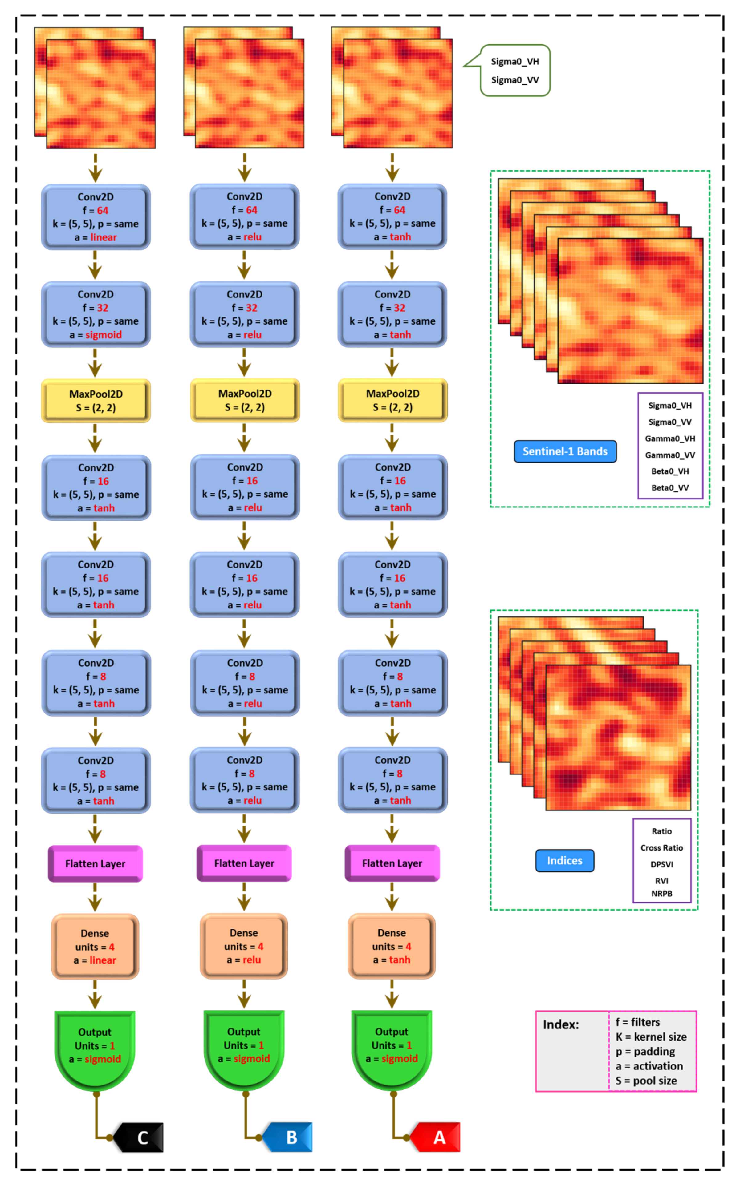
2.3. Model Establishment

A convolutional neural network (CNN) is useful for researchers. CNN is an invaluable and indispensable tool to deal with satellite images. In general, the CNN structure mainly consists of an input layer, one or more hidden layers, and an output layer. The hidden layers of a CNN are typically comprised of convolutional layers, nonlinearity layers, pooling layers, and fully connected layers. A convolution layer is responsible for feature extraction. A nonlinearity layer mainly consists of an activation function (activation functions used tanh, sigmoid, ReLU, and linear). Activation functions are a critical part of the design of the network. In the hidden layer, the activation function type controls how well the model learns the training dataset. In the output layer, the activation function type defines the type of predictions the model can make. The pooling layer works to reduce the size of the input images by keeping the most important features only. The output of convolution layers and pooling layers is the input to the fully connected layers to get the final output (prediction of soil moisture content). For more information on designing CNN structures, see [59,60].

The overarching goal was to create a CNN model capable of predicting or retrieving soil moisture from satellite imagery with high efficiency and accuracy. The harder, more important step involves identifying the best-performing architecture. Figure 1 illustrates the perfect design in terms of the number of layers used (this is a result of many attempts and tests), which are appropriate for this type of data. One of the most useful features of CNN is the possibility of using different activation functions for each layer. Based on this feature, we used three CNN architectures exactly alike (A, B, and C), except for the activation function, as shown in Figure 1.

No one can deny that there is a strong positive correlation between inputs, feature extraction processes, and outputs. CNN has tremendous potential to extract complex features. Accordingly, the next critical step was to select and determine the best inputs, which is done from Sentinel bands. The choice of the most suitable and appropriate activation functions for CNN will help to achieve better performance and the maximum score regression. We need to first identify the impact of each band on soil moisture retrieval. Many indices were used extensively with Sentinel-1 data. The most common are: cross-ratio ($CR={\sigma }_{VH}^0/{\sigma }_{VV}^0$) [61], Ratio ($Ratio={\sigma }_{VV}^0/{\sigma }_{VH}^0$) [62,63,64], radar vegetation index ($RVI=4{\sigma }_{VH}^0/\left({\sigma }_{VV}^0+{\sigma }_{VH}^0\right)$) [65,66], dual polarization SAR vegetation index ($DPSVI=\left({\sigma }_{VV}^0+{\sigma }_{VH}^0\right)/{\sigma }_{VV}^0$) [67,68,69], and normalized ratio procedure between bands ($NRPB=\left({\sigma }_{VH}^0-{\sigma }_{VV}^0\right)/\left({\sigma }_{VH}^0+{\sigma }_{VV}^0\right)$) [70,71,72]. We therefore need to know the impact of the use of these indices as input data to the CNN model on the soil moisture retrieval.

The total number of Sentinel-1 images used for running CNN is 17,325 images. During the fitting of the model, we split our dataset randomly into two parts: 80% for training and 20% for testing. Finally, coefficient of determination ($R^2$), mean absolute error ($MAE$), and root mean square error ($RMSE$) were used to estimate how good the performance of the prediction model was designed.

$$\begin{gathered} R^2=1-\frac{{{\displaystyle \sum }}_{i=1}^n{\left(y_i-{\widehat{y}}_i\right)}^2}{{{\displaystyle \sum }}_{i=1}^n{\left(y_i-\overline{y}\right)}^2} \\ MAE=\frac{1}{n}{\displaystyle \sum }_{i=1}^n\left|y_i-{\widehat{y}}_i\right| \\ RMSE=\sqrt{\frac{1}{n}{\displaystyle \sum }_{i=1}^n{\left(y_i-{\widehat{y}}_i\right)}^2} \end{gathered}$$

where ($y_i$) is the actual value, (${\widehat{y}}_i$) is the predicted value of ($y_i$), (${\overline{y}}_i$) is the mean of the ($y$) values, and ($n$) is the number of data points.

The modeling process was performed on a Windows workstation (Windows 10) with an Intel Xeon Gold 5218 Processors (16-Cores, 16M Cache), 128 GB of RAM, and an NVIDIA Quadro P4000 graphics cards (8 GB of RAM). CNN model building was implemented by using the python programming language. Python is an integrated, powerful, and flexible language. Moreover, it is easy to learn, write, and understand.

3. Results and Discussion

3.1. Influence of VH and VV Polarization as Input Data to the CNN Model on the Soil Moisture Retrieval

With this study, we found that the most appropriate CNN architecture for Sentinel-1 data are CNN architecture (C), as elaborated later in this paper. Therefore, we suffice with presenting its findings. Figure 2 summarizes the results obtained on Sentinel-1 bands, which were achieved by using the CNN model (CNN architecture (C)) proposed in this study. This figure illustrates the relationship between in-situ soil moisture and predicted soil moisture, clarifying R², MAE, and RMSE metrics, for (1) each band separately; (2) Sigma0_VH and Sigma0_VV; (3) Gamma0_VH and Gamma0_VV; (4) Beta0_VH and Beta0_VV; (5) all VH bands together; (6) all VV bands together; and (7) all VH and VV bands (6 bands).

In all, we noticed that VV bands were better than VH bands for soil moisture retrieval, but the best way is to use both at the same time (e.g., Sigma0_VH and Sigma0_VV). The coefficients of determination (R²) for Sigma0_VH, Gamma0_VH, and Beta0_VH are 0.8078, 0.8023, and 0.8002, respectively. Similarly, R² for Sigma0_VV, Gamma0_VV, and Beta0_VV are 0.8399, 0.8337, and 0.8323, respectively. With the use of both VH and VV bands, R² values have improved to 0.8664, 0.8554, and 0.8527 for Sigma0_VH and Sigma0_VV, Gamma0_VH and Gamma0_VV, and Beta0_VH and Beta0_VV, respectively. In the light of the current findings: Arguably, Sigma0, Gamma0, and Beta0 have the same influence on soil moisture estimation. In essence, Sigma0, Gamma0, or Beta0 can be used to predict soil moisture content, but the best is to use Sigma0. When comparing the result obtained from the use of all VH bands together with the result obtained from the use of each VH band separately, and between use of all VV bands together with the use of each VV band separately, we will find that (1) use of three bands (VH or VV) together causes a decrease in soil moisture retrieval efficiency; (2) the R² value has reduced to 0.777 with use all VH bands together; and (3) the R² value has reduced to 0.8152 with use all VV bands together. By using all VH and VV bands, the value of R² has amounted to 0.8277.

From the above, it will be clear that (1) soil moisture retrieval efficiency was good with 1 input channels (Sigma0_VH or Sigma0_VV or Gamma0_VH or Gamma0_VV or Beta0_VH or Beta0_VV); (2) it was further improved with 2 input channels (Sigma0_VH and Sigma0_VV or Gamma0_VH and Gamma0_VV or Beta0_VH and Beta0_VV); and (3) it was worsened with three input channels (all VH or VV bands) and with six input channels (all VH and VV bands).

To explain that, we must be fully aware that the machine learning algorithm’s accuracy depends on the quality of the input data [73,74]. Multiple studies reveal a positive correlation between the number of features and accuracy; that is until it peaks, but then it will turn to a negative correlation. The proper features can certainly increase the accuracy [75]. Redundant and irrelevant features may lead to confusion in the learning system [76]. Removing these features can help avoid degradation of learning performance [77].

We can convert from Beta naught (${\beta }^0$) to Sigma naught (${\sigma }^0$) or Gamma naught (${\gamma }^0$) by multiplying Beta naught by a specific number, as follows: (${\sigma }^0={\beta }^0\times \sin \theta$) and (${\gamma }^0={\beta }^0\times \tan \theta$), where ($\theta$) is the incidence angle [78,79]. We can therefore consider Sigma naught, Gamma naught, and Beta naught as mirror bands or mirror images or redundant images. The only differences are the minimum and maximum values of the backscattering coefficient. As a result, we notice that the values of the performance metrics for Sigma0_VH, Gamma0_VH, and Beta0_VH look the same. Moreover, the values of the performance metrics for Sigma0_VV, Gamma0_VV, and Beta0_VV look the same.

When we use all VH bands together as input data, the Gamma and Beta could be regarded as redundant features of Sigma. Similarly, this also applies to the use of all VV bands together as input data. Hence, we believe that redundant features were the main reason for the degradation of the performance metrics (R², MAE, and RMSE) with the use of all VH bands together, all VV bands together, and both VH and VV bands; in comparison with the values of the performance metrics for each band separately, Sigma0_VH and Sigma0_VV, Gamma0_VH and Gamma0_VV, and Beta0_VH and Beta0_VV.

3.2. Influence of Cross-Ratio, Ratio, RVI, NRPB and DPSVI as Input Data to the CNN Model on the Soil Moisture Retrieval

Figure 3 summarizes the findings obtained from the use of indicators as input data to the CNN. The best indicators for soil moisture retrieval is Cross-Ratio ($R^2=0.7436$), followed by Ratio ($R^2=0.743$), then DPSVI ($R^2=0.741$), followed by RVI ($R^2=0.7351$), and finally NRPB ($R^2=0.7346$). The values of the coefficients of determination for indicators ranging from 0.7436 to 0.7346. One explanation for this tiny range of the difference is that all the indicators depended only on Sigma0, as illustrated earlier by the equations.

As shown in Figure 3, there are substantial declines in the values of the performance metrics ($R^2=0.6965, MAE=0.025, RMSE=0.0414$), due to using all indicators as input to the CNN. Moreover, the use of all Sentinel-1 bands and indicators together (six bands and five indicators) as input data to the CNN instead of using all Sentinel-1 bands, led to a decline in the values of the performance metrics from ($R^2=0.8277, MAE=0.0194, RMSE=0.0312$) to ($R^2=0.7973, MAE=0.0238, RMSE=0.0338$). All of this confirms what has been interpreted regarding the impact of redundant features on learning performance.

According to these results, the use of indicators instead of original Sentinel-1 bands as input data to the CNN to retrieve soil moisture from Sentinel-1 images is not recommended. We can now say that the top three inputs to CNN are Sigma0_VH and Sigma0_VV, Gamma0_VH and Gamma0_VV, and Beta0_VH and Beta0_VV. However, the best of all is Sigma0_VH and Sigma0_VV.

3.3. The Impact of the Activation Function

As mentioned earlier, we will be using the three CNN architectures, and the only difference between them is the activation function, as seen in Figure 1. Now we will use the top three inputs with three CNN architectures, to select the best CNN architecture (or more specifically, the best activation function).

Figure 4 summarizes and illustrates the effect of changing the activation function on learning performance. The best results had already been achieved by CNN architecture (C). While CNN architecture (B) had produced bad or modest results. The main drawback is that it is insensitive to high moisture. The maximum value of soil moisture, which CNN architecture (B) can sense or predict it is ($0.603 {\mathrm{m}}^3/{\mathrm{m}}^3$). With using the CNN architecture (B), the values of the performance metrics have decreased to ($R^2=0.8381, MAE=0.0164, RMSE=0.0302$), ($R^2=0.8311, MAE=0.0169, RMSE=0.0309$), and ($R^2=0.8288, MAE=0.0164, RMSE=0.0311$) for Sigma0_VH and Sigma0_VV, Gamma0_VH and Gamma0_VV, and Beta0_VH and Beta0_VV, respectively. Concerning the CNN architecture (A), it provided good results, slightly better than the results of the CNN architecture (B). However, we do not recommend the use of this architecture at all. His sensitivity to low moisture is fairly weak. CNN architecture (A) cannot sense or predict soil moisture less than ($0.1509 {\mathrm{m}}^3/{\mathrm{m}}^3$). The weird stuff, which we encountered during the use of the CNN architecture (A), is that this architecture is sometimes unable to learn anything. When this happened, we noticed that the loss value had always been the same (immutable value), as of epoch 3 during training. Then we re-trained the model again from the beginning. Amazingly, we already have these results: ($R^2=0.8454, MAE=0.0161, RMSE=0.0295$), ($R^2=0.8427, MAE=0.0168, RMSE=0.0298$), and ($R^2=0.836, MAE=0.0172, RMSE=0.0304$) for Sigma0_VH and Sigma0_VV, Gamma0_VH and Gamma0_VV, and Beta0_VH and Beta0_VV, respectively. To be honest, we do not have any explanation for this. Ultimately, the best architecture that fits these kinds of data is CNN architecture (C).

3.4. Comparison between CNN Architecture ($C\left(II\right)$) and CNN Architecture ($C\left(III\right)$)

However, after knowing the best inputs to the CNN and the most appropriate activation functions, we will try to illustrate the impact of change in the number of convolutional layers as well as the number of filters in a convolution layer, while taking into account the need to preserve the same pattern of activation functions for CNN architecture (C). Accordingly, two new architectures were presented, called CNN architecture ($\mathrm{C}\left(\mathrm{II}\right)$) and CNN architecture ($\mathrm{C}\left(\mathrm{III}\right)$), as shown in Figure 5.

Figure 6 displays the magnitude of the influence of these two new architectures on the values of the performance metrics. Decreasing the number of convolutional layers, as well as the number of filters in a convolution layer, has harmed the efficiency of the CNN model. There is a significant reduction in performance metrics as a result of the use of the CNN architecture ($\mathrm{C}\left(\mathrm{III}\right)$): from ($R^2=0.8664, MAE=0.0144, RMSE=0.0274$), ($R^2=0.8554, MAE=0.0159, RMSE=0.0285$), and ($R^2=0.8527, MAE=0.017, RMSE=0.0288$) to ($R^2=0.8037, MAE=0.0205, RMSE=0.0333$), ($R^2=0.7995, MAE=0.0214, RMSE=0.0336$), and ($R^2=0.7952, MAE=0.022, RMSE=0.034$) for Sigma0_VH and Sigma0_VV, Gamma0_VH and Gamma0_VV, and Beta0_VH and Beta0_VV, respectively. Due to the usage of the CNN architecture ($\mathrm{C}\left(\mathrm{II}\right)$), plunged further to about ($R^2=0.5465, MAE=0.0392, RMSE=0.0506$), ($R^2=0.5384, MAE=0.0394, RMSE=0.051$), and ($R^2=0.5307, MAE=0.0396, RMSE=0.0514$) for Sigma0_VH and Sigma0_VV, Gamma0_VH and Gamma0_VV, and Beta0_VH and Beta0_VV, respectively.

We can now say with high confidence that: (1) VV polarization is more sensitive than VH polarization for soil moisture retrieval; similar results have been found by [19,20,21,22,23]. (2) The combination of VV and VH polarization has resulted in improvement in the prediction of soil moisture from Sentinel-1 images, our result agree with [24,25,26]. (3) The best inputs to the CNN to retrieve soil moisture from Sentinel-1 images are Sigma0_VH and Sigma0_VV, or Gamma0_VH and Gamma0_VV, or Beta0_VH and Beta0_VV. (4) The most appropriate CNN architecture for Sentinel-1 data are CNN architecture (C) (especially, the activation function style). (5) We need to use twice or three times the number of Sentinel-1 images used in this paper, to improve this model and make it more precise as the precision of field measurements. We will attempt to demonstrate and prove this in future research.

4. Conclusions

Agriculture is closely linked to food, water, and air. Smart agriculture is a “ray of hope” for food, water, and environmental security. Satellites and artificial intelligence are necessary tools to achieve smart agriculture. Due to rapid technological development in our time and an increase in the number of satellites, we will soon be able to obtain high spatial resolution images of the Earth once or twice a day. Artificial intelligence can analyze and understand a large amount of data effectively and efficiently.

Soil moisture content is one of the decisive conditions required for crop growth and development and its precise prediction is important for determining when to irrigate and how much water to apply; this helps avoid problems associated with over- and under-watering. This also contributes to an increase in areas cultivated and, hence, agricultural productivity and air purification. Gravimetric, neutron probe, TDR probe, FDR probe, tensiometer probe technique are the most common techniques used for estimating soil moisture content in situ. All of these techniques under field conditions are accurate with varying degrees. However, the most common challenges and problems that still exist with these techniques under field conditions are (1) point measurement methods; (2) regular periodic maintenance, thus require intensive labor; (3) the need for site-specific calibration; (4) the actual contact with the soil; (5) the costs.

Therefore, in this paper, we proposed a new approach to detect moisture content in soil without actually being in contact with it. We propose a convolutional neural network (CNN) architecture that can predict soil moisture content over agricultural areas from Sentinel-1 images. The best values of the performance metrics ($R^2=0.8664, MAE=0.0144, RMSE=0.0274$) were achieved as a result of using Sigma0_VH and Sigma0_VV as input to the CNN architecture (C). The pre-processing steps have a strong, effective, and direct influence on soil moisture retrieval from Sentinel-1 images. Using VV bands as input data to the CNN is better than using VH bands for soil moisture retrieval. The use of indicators instead of original Sentinel-1 bands as input data to the CNN to retrieve soil moisture from Sentinel-1 images is not recommended. We recommend using Sigma0_VH and Sigma0_VV or Gamma0_VH and Gamma0_VV or Beta0_VH and Beta0_VV as input data to the CNN to predict soil moisture content from Sentinel-1 images.

References

1. Fedoroff, N.V.J.A.; Security, F. Food in a future of 10 billion. Agric. Food Secur. 2015, 4, 1–10. [Google Scholar] [CrossRef] [Green Version]
2. Department of Economic and Social Affairs, United Nations. Population Division. World Population Prospects: The 2015 Revision, Key Findings and Advance Tables. In Working Paper No. ESA/P/WP.241; Department of Economic and Social Affairs, United Nations: New York, NY, USA, 2015; pp. 1–66. [Google Scholar]
3. Shukla, A.; Panchal, H.; Mishra, M.; Patel, P.; Srivastava, H.; Patel, P.; Shukla, A. Soil moisture estimation using gravimetric technique and FDR probe technique: A comparative analysis. Am. Int. J. Res. Formal Appl. Nat. Sci. 2014, 8, 89–92. [Google Scholar]
4. Maltese, A.; Capodici, F.; Ciraolo, G.; Loggia, G.L. Soil water content assessment: Critical issues concerning the operational application of the triangle method. Sensors 2015, 15, 6699–6718. [Google Scholar] [CrossRef]
5. Aguilar, J.; Rogers, D.; Kisekka, I. Irrigation scheduling based on soil moisture sensors and evapotranspiration. Kans. Agric. Exp. Stn. Res. Rep. 2015, 1, 20. [Google Scholar] [CrossRef] [Green Version]
6. Jones, H.G. Irrigation scheduling: Advantages and pitfalls of plant-based methods. J. Exp. Bot. 2004, 55, 2427–2436. [Google Scholar] [CrossRef] [Green Version]
7. Ahmed, A.; Zhang, Y.; Nichols, S. Review and evaluation of remote sensing methods for soil-moisture estimation. SPIE Rev. 2011, 2, 028001. [Google Scholar]
8. Yoder, R.; Johnson, D.; Wilkerson, J.; Yoder, D. Soilwater sensor performance. Appl. Eng. Agric. 1998, 14, 121–133. [Google Scholar] [CrossRef]
9. Liang, S.; Wang, J. Advanced Remote Sensing: Terrestrial Information Extraction and Applications; Academic Press: Cambridge, MA, USA, 2019. [Google Scholar]
10. Zeng, L.; Hu, S.; Xiang, D.; Zhang, X.; Li, D.; Li, L.; Zhang, T. Multilayer soil moisture mapping at a regional scale from multisource data via a machine learning method. Remote Sens. 2019, 11, 284. [Google Scholar] [CrossRef] [Green Version]
11. Ford, T.; Harris, E.; Quiring, S. Estimating root zone soil moisture using near-surface observations from SMOS. Hydrol. Earth Syst. Sci. 2014, 18, 139–154. [Google Scholar] [CrossRef] [Green Version]
12. Muller, E.; Decamps, H. Modeling soil moisture–reflectance. Remote Sens. Environ. 2001, 76, 173–180. [Google Scholar] [CrossRef] [Green Version]
13. Ulaby, F.; Long, D. Microwave Radar and Radiometric Remote Sensing; Artech House: Norwood, MA, USA, 2015. [Google Scholar]
14. Woodhouse, I.H. Introduction to Microwave Remote Sensing; CRC Press: Boca Raton, FL, USA, 2017. [Google Scholar]
15. Singh, V.P.; Singh, P.; Haritashya, U.K. Encyclopedia of Snow, Ice and Glaciers; Springer: Dordrecht, The Netherlands, 2011. [Google Scholar]
16. Njoku, E.G.; Kong, J.A. Theory for passive microwave remote sensing of near-surface soil moisture. J. Geophys. Res. 1977, 82, 3108–3118. [Google Scholar] [CrossRef]
17. Bourgeau-Chavez, L.L.; Kasischke, E.S.; Riordan, K.; Brunzell, S.; Nolan, M.; Hyer, E.; Slawski, J.; Medvecz, M.; Walters, T.; Ames, S. Remote monitoring of spatial and temporal surface soil moisture in fire disturbed boreal forest ecosystems with ERS SAR imagery. Int. J. Remote Sens. 2007, 28, 2133–2162. [Google Scholar] [CrossRef]
18. Dobson, M.C.; Ulaby, F.T. Active microwave soil moisture research. IEEE Trans. Geosci. Remote Sens. 1986, GE-24, 23–36. [Google Scholar] [CrossRef]
19. El Hajj, M.; Baghdadi, N.; Zribi, M.; Bazzi, H. Synergic use of Sentinel-1 and Sentinel-2 images for operational soil moisture mapping at high spatial resolution over agricultural areas. Remote Sens. 2017, 9, 1292. [Google Scholar] [CrossRef] [Green Version]
20. Li, Y.; Zhang, C.; Heng, W. Retrieving Surface Soil Moisture over Wheat-Covered Areas Using Data from Sentinel-1 and Sentinel-2. Water 2021, 13, 1981. [Google Scholar] [CrossRef]
21. Bousbih, S.; Zribi, M.; Lili-Chabaane, Z.; Baghdadi, N.; El Hajj, M.; Gao, Q.; Mougenot, B.J.S. Potential of Sentinel-1 radar data for the assessment of soil and cereal cover parameters. Sensors 2017, 17, 2617. [Google Scholar] [CrossRef] [PubMed] [Green Version]
22. Ezzahar, J.; Ouaadi, N.; Zribi, M.; Elfarkh, J.; Aouade, G.; Khabba, S.; Er-Raki, S.; Chehbouni, A.; Jarlan, L.J.R.S. Evaluation of backscattering models and support vector machine for the retrieval of bare soil moisture from Sentinel-1 data. Remote Sens. 2020, 12, 72. [Google Scholar] [CrossRef] [Green Version]
23. Sutariya, S.; Hirapara, A.; Meherbanali, M.; Tiwari, M.; Singh, V.; Kalubarme, M. Soil Moisture Estimation using Sentinel-1 SAR data and Land Surface Temperature in Panchmahal district, Gujarat State. Int. J. Environ. Geoinform. 2021, 8, 65–77. [Google Scholar] [CrossRef]
24. Ayehu, G.; Tadesse, T.; Gessesse, B.; Yigrem, Y.J.R.S. Soil moisture monitoring using remote sensing data and a stepwise-cluster prediction model: The case of Upper Blue Nile Basin, Ethiopia. Remote Sens. 2019, 11, 125. [Google Scholar] [CrossRef] [Green Version]
25. Hoskera, A.K.; Nico, G.; Irshad Ahmed, M.; Whitbread, A.J.R.S. Accuracies of soil moisture estimations using a semi-empirical model over bare soil agricultural croplands from sentinel-1 SAR data. Remote Sens. 2020, 12, 1664. [Google Scholar] [CrossRef]
26. Liu, C. Analysis of Sentinel-1 SAR Data for Mapping Standing Water in the Twente Region. Master’s Thesis, University of Twente, Enschede, The Netherlands, 2016. [Google Scholar]
27. Hu, Y.; Li, W.; Wright, D.; Aydin, O.; Wilson, D.; Maher, O.; Raad, M. Artificial intelligence approaches. arXiv 2019, arXiv:1908.10345. (preprint). [Google Scholar] [CrossRef] [Green Version]
28. Grewal, D.S. A critical conceptual analysis of definitions of artificial intelligence as applicable to computer engineering. IOSR J. Comput. Eng. 2014, 16, 9–13. [Google Scholar] [CrossRef]
29. Hardian, R.; Liang, Z.; Zhang, X.; Szekely, G. Artificial intelligence: The silver bullet for sustainable materials development. Green Chem. 2020, 22, 7521–7528. [Google Scholar] [CrossRef]
30. Schmidt-Erfurth, U.; Sadeghipour, A.; Gerendas, B.S.; Waldstein, S.M.; Bogunović, H. Artificial intelligence in retina. Prog. Retin. Eye Res. 2018, 67, 1–29. [Google Scholar] [CrossRef] [PubMed]
31. Robert, N. How artificial intelligence is changing nursing. Nurs. Manag. 2019, 50, 30. [Google Scholar] [CrossRef]
32. LeCun, Y.; Bengio, Y.; Hinton, G. Deep learning. Nature 2015, 521, 436–444. [Google Scholar] [CrossRef]
33. Yamashita, R.; Nishio, M.; Do, R.K.G.; Togashi, K. Convolutional neural networks: An overview and application in radiology. Insights Imaging 2018, 9, 611–629. [Google Scholar] [CrossRef] [Green Version]
34. Shaheen, F.; Verma, B.; Asafuddoula, M. Impact of automatic feature extraction in deep learning architecture. In Proceedings of the 2016 International Conference on Digital Image Computing: Techniques and Applications (DICTA), Gold Coast, Australia, 30 November–2 December 2016; pp. 1–8. [Google Scholar]
35. Galib, S.M. Applications of Machine Learning in Nuclear Imaging and Radiation Detection; Missouri University of Science and Technology: Rolla, MO, USA, 2019. [Google Scholar]
36. Zhu, X.X.; Tuia, D.; Mou, L.; Xia, G.-S.; Zhang, L.; Xu, F.; Fraundorfer, F. Deep learning in remote sensing: A comprehensive review and list of resources. IEEE Geosci. Remote. Sens. Mag. 2017, 5, 8–36. [Google Scholar] [CrossRef] [Green Version]
37. Andrearczyk, V.; Whelan, P.F. Deep learning in texture analysis and its application to tissue image classification. In Biomedical Texture Analysis; Elsevier: Amsterdam, The Netherlands, 2017; pp. 95–129. [Google Scholar]
38. Mahmood, A.; Bennamoun, M.; An, S.; Sohel, F.; Boussaid, F.; Hovey, R.; Kendrick, G.; Fisher, R.B. Deep learning for coral classification. In Handbook of Neural Computation; Elsevier: Amsterdam, The Netherlands, 2017; pp. 383–401. [Google Scholar]
39. Perez, D.; Islam, K.; Hill, V.; Zimmerman, R.; Schaeffer, B.; Shen, Y.; Li, J. Quantifying seagrass distribution in coastal water with deep learning models. Remote Sens. 2020, 12, 1581. [Google Scholar] [CrossRef]
40. Hu, Z.; Xu, L.; Yu, B. Soil Moisture Retrieval Using Convolutional Neural Networks: Application to Passive Microwave Remote Sensing. Int. Arch. Photogramm. Remote Sens. Spat. Inf. Sci. 2018, 42. [Google Scholar] [CrossRef] [Green Version]
41. Dorigo, W.; Wagner, W.; Hohensinn, R.; Hahn, S.; Paulik, C.; Xaver, A.; Gruber, A.; Drusch, M.; Mecklenburg, S.; van Oevelen, P. International Soil Moisture Network: A Data Hosting Facility for Global in Situ Soil Moisture Measurements. Hydrol. Earth Syst. Sci. 2011, 15, 1675–1698. [Google Scholar] [CrossRef] [Green Version]
42. Dorigo, W.; Xaver, A.; Vreugdenhil, M.; Gruber, A.; Hegyiova, A.; Sanchis-Dufau, A.; Zamojski, D.; Cordes, C.; Wagner, W.; Drusch, M. Global automated quality control of in situ soil moisture data from the International Soil Moisture Network. Vadose Zone J. 2013, 12, 1–21. [Google Scholar] [CrossRef]
43. Aberer, D.; Himmelbauer, I.; Schremmer, L.; Petrakovic, I.; Dorigo, W.; Goryl, P.; Sabia, R. The International Soil Moisture Network in assistance of EO soil moisture validation products, services and models. In Proceedings of the EGU General Assembly Conference Abstracts, Vienna, Austria, 4–8 May 2020; p. 16493. [Google Scholar]
44. Smith, A.B.; Walker, J.P.; Western, A.W.; Young, R.; Ellett, K.; Pipunic, R.; Grayson, R.; Siriwardena, L.; Chiew, F.H.; Richter, H. The Murrumbidgee soil moisture monitoring network data set. Water Resour. Res. 2012, 48, 1–6. [Google Scholar] [CrossRef]
45. Young, R.; Walker, J.; Yeoh, N.; Smith, A.; Ellett, K.; Merlin, O.; Western, A. Soil Moisture and Meteorological Observations from the Murrumbidgee Catchment; Department of Civil and Environmental Engineering, The University of Melbourne: Melbourne, Australia, 2008. [Google Scholar]
46. Foelsche, U. Assessment of spatial uncertainty of heavy rainfall at catchment scale using a dense gauge network. Hydrol. Earth Syst. Sci. 2019, 23, 2863–2875. [Google Scholar]
47. Fuchsberger, J.; Kirchengast, G.; Kabas, T. Release Notes for Version 7 of the WegenerNet Processing System (WPS Level-2 Data v7); Wegener Center for Climate and Global Change, University of Graz: Graz, Austria, 2018. [Google Scholar]
48. Kabas, T. WegenerNet Klimastationsnetz Region Feldbach: Experimenteller Aufbau und Hochauflösende Daten für die Klima-und Umweltforschung. Ph.D. Thesis, University of Graz, Graz, Austria, 2011. [Google Scholar]
49. Kirchengast, G.; Kabas, T.; Leuprecht, A.; Bichler, C.; Truhetz, H. Wegenernet: A pioneering high-resolution network for monitoring weather and climate. Bull. Am. Meteorol. Soc. 2014, 95, 227–242. [Google Scholar] [CrossRef]
50. Potin, P.; Rosich, B.; Miranda, N.; Grimont, P.; Shurmer, I.; O’Connell, A.; Krassenburg, M.; Gratadour, J.-B. Copernicus Sentinel-1 Constellation Mission Operations Status. In Proceedings of the IGARSS 2019-2019 IEEE International Geoscience and Remote Sensing Symposium, Yokohama, Japan, 28 July–2 August 2019; pp. 5385–5388. [Google Scholar]
51. Abdikan, S.; Sanli, F.B.; Ustuner, M.; Calò, F. Land cover mapping using sentinel-1 SAR data. Int. Arch. Photogramm. Remote Sens. Spat. Inf. Sci. 2016, 41, 757. [Google Scholar] [CrossRef] [Green Version]
52. Bovenga, F.; Belmonte, A.; Refice, A.; Pasquariello, G.; Nutricato, R.; Nitti, D.O.; Chiaradia, M.T. Performance analysis of satellite missions for multi-temporal SAR interferometry. Sensors 2018, 18, 1359. [Google Scholar] [CrossRef] [PubMed] [Green Version]
53. Van Tricht, K.; Gobin, A.; Gilliams, S.; Piccard, I. Synergistic use of radar Sentinel-1 and optical Sentinel-2 imagery for crop mapping: A case study for Belgium. Remote Sens. 2018, 10, 1642. [Google Scholar] [CrossRef] [Green Version]
54. Baghdadi, N.; El Hajj, M.; Zribi, M. An operational high resolution soil moisture retrieval algorithm using sentinel-1 images. In Proceedings of the 2019 PhotonIcs & Electromagnetics Research Symposium-Spring (PIERS-Spring), Rome, Italy, 17–20 June 2019; pp. 4086–4092. [Google Scholar]
55. Carreiras, J.M.; Quegan, S.; Tansey, K.; Page, S. Sentinel-1 observation frequency significantly increases burnt area detectability in tropical SE Asia. Environ. Res. Lett. 2020, 15, 054008. [Google Scholar] [CrossRef]
56. Gao, Q.; Zribi, M.; Escorihuela, M.J.; Baghdadi, N. Synergetic use of Sentinel-1 and Sentinel-2 data for soil moisture mapping at 100 m resolution. Sensors 2017, 17, 1966. [Google Scholar] [CrossRef] [PubMed] [Green Version]
57. Ticehurst, C.; Zhou, Z.-S.; Lehmann, E.; Yuan, F.; Thankappan, M.; Rosenqvist, A.; Lewis, B.; Paget, M. Building a SAR-Enabled Data Cube Capability in Australia Using SAR Analysis Ready Data. Data 2019, 4, 100. [Google Scholar] [CrossRef] [Green Version]
58. Mouche, A.; Chapron, B. Global C-B and E nvisat, RADARSAT-2 and S entinel-1 SAR measurements in copolarization and cross-polarization. J. Geophys. Res. Ocean. 2015, 120, 7195–7207. [Google Scholar] [CrossRef] [Green Version]
59. Khan, S.; Rahmani, H.; Shah, S.A.A.; Bennamoun, M.; Medioni, G.; Dickinson, S. A Guide to Convolutional Neural Networks for Computer Vision. In Synthesis Lectures on Computer Vision; Morgan & Claypool: San Rafael, CA, USA, 2018; Volume 8, pp. 1–207. [Google Scholar]
60. Sewak, M.; Karim, M.R.; Pujari, P. Practical Convolutional Neural Networks: Implement. Advanced Deep Learning Models Using Python; Packt Publishing Ltd.: Birmingham, UK, 2018. [Google Scholar]
61. Vreugdenhil, M.; Wagner, W.; Bauer-Marschallinger, B.; Pfeil, I.; Teubner, I.; Rüdiger, C.; Strauss, P. Sensitivity of Sentinel-1 backscatter to vegetation dynamics: An Austrian case study. Remote Sens. 2018, 10, 1396. [Google Scholar] [CrossRef] [Green Version]
62. Dabrowska-Zielinska, K.; Musial, J.; Malinska, A.; Budzynska, M.; Gurdak, R.; Kiryla, W.; Bartold, M.; Grzybowski, P. Soil moisture in the Biebrza Wetlands retrieved from Sentinel-1 imagery. Remote Sens. 2018, 10, 1979. [Google Scholar] [CrossRef] [Green Version]
63. Frison, P.-L.; Fruneau, B.; Kmiha, S.; Soudani, K.; Dufrene, E.; Le Toan, T.; Koleck, T.; Villard, L.; Mougin, E.; Rudant, J.-P. Potential of Sentinel-1 data for monitoring temperate mixed forest phenology. Remote Sens. 2018, 10, 2049. [Google Scholar] [CrossRef] [Green Version]
64. Hardy, A.; Ettritch, G.; Cross, D.E.; Bunting, P.; Liywalii, F.; Sakala, J.; Silumesii, A.; Singini, D.; Smith, M.; Willis, T. Automatic detection of open and vegetated water bodies using Sentinel 1 to map African malaria vector mosquito breeding habitats. Remote Sens. 2019, 11, 593. [Google Scholar] [CrossRef] [Green Version]
65. Holtgrave, A.-K.; Röder, N.; Ackermann, A.; Erasmi, S.; Kleinschmit, B. Comparing Sentinel-1 and-2 Data and Indices for Agricultural Land Use Monitoring. Remote Sens. 2020, 12, 2919. [Google Scholar] [CrossRef]
66. Kim, Y.; van Zyl, J.J. A time-series approach to estimate soil moisture using polarimetric radar data. IEEE Trans. Geosci. Remote Sens. 2009, 47, 2519–2527. [Google Scholar]
67. Mandal, D.; Kumar, V.; Ratha, D.; Dey, S.; Bhattacharya, A.; Lopez-Sanchez, J.M.; McNairn, H.; Rao, Y.S. Dual polarimetric radar vegetation index for crop growth monitoring using sentinel-1 SAR data. Remote Sens. Environ. 2020, 247, 111954. [Google Scholar] [CrossRef]
68. Periasamy, S. Significance of dual polarimetric synthetic aperture radar in biomass retrieval: An attempt on Sentinel-1. Remote Sens. Environ. 2018, 217, 537–549. [Google Scholar] [CrossRef]
69. Periasamy, S.; Senthil, D.; Shanmugam, R.S. A Modified Triangle with SAR Target Parameters for Soil Texture Categorization Mapping. In Proceedings of the Conference of the Arabian Journal of Geosciences, Sousse, Tunisia, 12–15 November 2018; pp. 97–99. [Google Scholar]
70. Filgueiras, R.; Mantovani, E.C.; Althoff, D.; Fernandes Filho, E.I.; da Cunha, F.F. Crop NDVI monitoring based on sentinel 1. Remote Sens. 2019, 11, 1441. [Google Scholar] [CrossRef] [Green Version]
71. Mohite, J.; Sawant, S.; Pandit, A.; Pappula, S. Investigating the Performance of Random Forest and Support Vector Regression for Estimation of Cloud-Free Ndvi Using SENTINEL-1 SAR Data. Int. Arch. Photogramm. Remote Sens. Spat. Inf. Sci. 2020, 43, 1379–1383. [Google Scholar] [CrossRef]
72. Sun, L.; Chen, J.; Guo, S.; Deng, X.; Han, Y. Integration of Time Series Sentinel-1 and Sentinel-2 Imagery for Crop Type Mapping over Oasis Agricultural Areas. Remote Sens. 2020, 12, 158. [Google Scholar] [CrossRef] [Green Version]
73. Sessions, V.; Valtorta, M. The Effects of Data Quality on Machine Learning Algorithms. ICIQ 2006, 6, 485–498. [Google Scholar]
74. Varma Rudraraju, N.; Boyanapally, V. Data Quality Model for Machine Learning. Master Thesis, Faculty of Computing, Blekinge Institute of Technology, Karlskrona, Sweden, 2019. [Google Scholar]
75. Pristyanto, Y.; Adi, S.; Sunyoto, A. The effect of feature selection on classification algorithms in credit approval. In Proceedings of the 2019 International Conference on Information and Communications Technology (ICOIACT), Yogyakarta, Indonesia, 24–25 July 2019; pp. 451–456. [Google Scholar]
76. Wang, S.; Tang, J.; Liu, H. Feature Selection. In Encyclopedia of Machine Learning and Data Mining; Springer Science & Business Media: New York, NY, USA, 2017. [Google Scholar]
77. Li, J.; Cheng, K.; Wang, S.; Morstatter, F.; Trevino, R.P.; Tang, J.; Liu, H. Feature selection: A data perspective. ACM Comput. Surv. (CSUR) 2017, 50, 1–45. [Google Scholar] [CrossRef] [Green Version]
78. Small, D. Flattening gamma: Radiometric terrain correction for SAR imagery. IEEE Trans. Geosci. Remote Sens. 2011, 49, 3081–3093. [Google Scholar] [CrossRef]
79. Ulander, L.M. Radiometric slope correction of synthetic-aperture radar images. IEEE Trans. Geosci. Remote Sens. 1996, 34, 1115–1122. [Google Scholar] [CrossRef]
Figure 1. An overview of a convolutional neural network (CNN) architecture.
Remotesensing 13 04964 g001
Figure 2. An illustration of the effect of Sentinel-1 bands on the soil moisture retrieval accuracy over agricultural areas.
Remotesensing 13 04964 g002
Figure 3. An illustration of the effect of indices used on the soil moisture retrieval accuracy over agricultural areas.
Remotesensing 13 04964 g003
Figure 4. The prediction performance of the CNN architecture (A), CNN architecture (B), and CNN architecture (C).
Remotesensing 13 04964 g004
Figure 5. Design ( C ( II ) ) and design ( C ( III ) ) of convolutional neural network.
Remotesensing 13 04964 g005
Figure 6. Validation accuracy for CNN architecture ( C ( II ) ) vs. validation accuracy for CNN architecture ( C ( III ) ).
Remotesensing 13 04964 g006