A Semi-Automatic Workflow to Extract Irregularly Aligned Plots and Sub-Plots: A Case Study on Lentil Breeding Populations

Abstract

Plant breeding experiments typically contain a large number of plots, and obtaining phenotypic data is an integral part of most studies. Image-based plot-level measurements may not always produce adequate precision and will require sub-plot measurements. To perform image analysis on individual sub-plots, they must be segmented from plots, other sub-plots, and surrounding soil or vegetation. This study aims to introduce a semi-automatic workflow to segment irregularly aligned plots and sub-plots in breeding populations. Imagery from a replicated lentil diversity panel phenotyping experiment with 324 populations was used for this study. Image-based techniques using a convolution filter on an excess green index (ExG) were used to enhance and highlight plot rows and, thus, locate the plot center. Multi-threshold and watershed segmentation were then combined to separate plants, ground, and sub-plot within plots. Algorithms of local maxima and pixel resizing with surface tension parameters were used to detect the centers of sub-plots. A total of 3489 reference data points was collected on 30 random plots for accuracy assessment. It was found that all plots and sub-plots were successfully extracted with an overall plot extraction accuracy of 92%. Our methodology addressed some common issues related to plot segmentation, such as plot alignment and overlapping canopies in the field experiments. The ability to segment and extract phenometric information at the sub-plot level provides opportunities to improve the precision of image-based phenotypic measurements at field-scale.

1. Introduction

Breeding programs screen thousands of progeny from parental crosses to select the desired phenotypic traits in new crop varieties. Phenometric information collected manually during the growing season is costly, labor-intensive, and subject to observer bias and error. Image-based plant phenotyping using unpiloted aerial vehicles (UAVs) offers a new opportunity for monitoring and extracting plant phenotypic information over time [1,2].

Image-based plant phenotyping requires that images be segmented into plots and sub-plots to analyze individual genotypes within a given experiment. Early generation breeding plots are often small and variable in size and location because of seed availability and seeder design limitations. Under field conditions, irregular patterns of plant growth caused by certain crops, genotype, and environment variation make the plot segmentation more challenging. Furthermore, sub-plot segmentation may be needed when higher phenotypic precision is required to avoid weed growth interference within the plots. Boundary extraction is an initial step to separate sub-plots within a plot. The plot extraction techniques include manual digitizing, field map-based, machine learning, and image-based. Among those, plot extraction using manual head-up digitizing [3,4] and field map-based techniques are common [5,6]. Although these approaches are accurate, manual adjustments are required, which is laborious. In the field map-based approach, plots are located based on a fixed distance between plots or ranges [6]. This is not always the case for large breeding experiments, where plot locations might be altered by seeding equipment and image distortions in the mosaicking process [7]. Region-based convolutional neural network (CNN) detection algorithm or simple CNN [8] shows high potential for large and closely packed trees, such as citrus or palm trees [9,10]. However, this method does not perform well on small plants with low ground cover and minimum distance between them [11]. Image-based methods relying on object-based or pixel-based classification [12,13] use vegetation indices or image pattern enhancements and require post-processing (after classification) to refine detected objects [8,14]. Although this method requires a low number of samples to conduct classification, post-processing is required to refine the result [6] and has high potential for delineation of irregularly spaced plots in a field [15]. Gaussian blob detection and random walker image segmentation have been proposed to segment lentil plots within a python-based workflow. This automatic process allows one to locate lentil blobs or plots automatically, but it is limited in merging plots which have grown together, and sub-plot separation [16].

This paper aimed to introduce a semi-automatic workflow to segment irregularly spaced plots and sub-plots in breeding populations. A lentil (Lens culinaris L.) plant breeding experiment was used to develop and demonstrate the applicability of this method to automatically segment irregularly spaced plots and sub-plots of a small crop.

2. Material and Methods

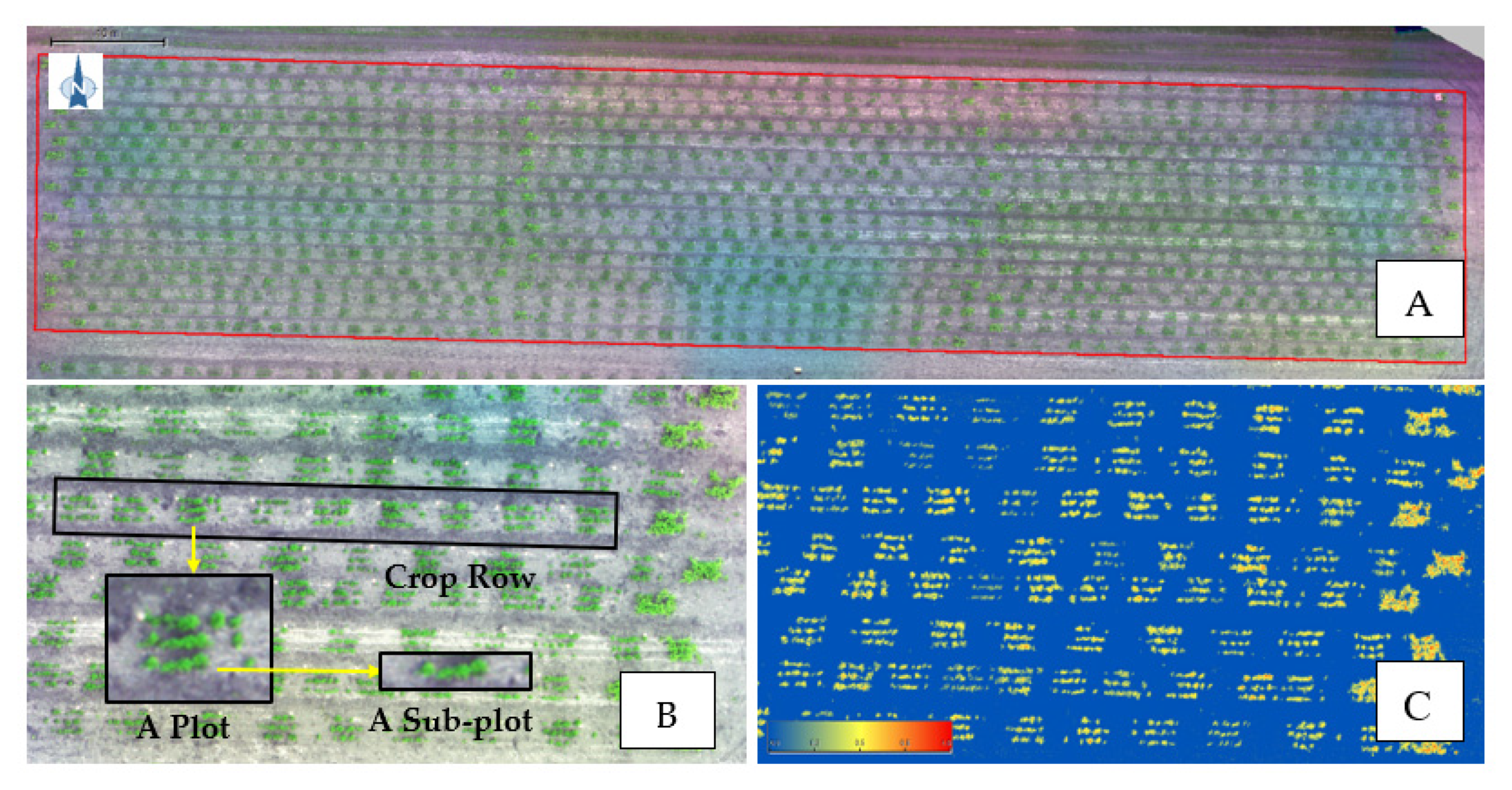
2.1. Field Study

The imagery for the study was obtained from a lentil diversity panel phenotyping experiment conducted at the Sutherland location of Kernen Crop Research Farm, Saskatoon, SK in 2018. A total of 324 lentil genotypes were distributed in a randomized lattice square (18 × 18) design with three replications. Each replicate was separated by a row of pea plots. The trial was seeded on 9 May 2018, with individual genotypes planted in 1 × 1 m plots following a seed rate of 60 seeds/plot and with a row spacing of 30 cm, resulting in three crop rows per plot. Each of the three rows constituting a plot was considered a sub-plot. The plots were sown using a tractor and seeder equipped with a GPS-guided auto-steering mechanism to align the crop rows. The inter-plot distance in the direction of seeder travel was inconsistent as the operator manually tripped the seeder to approximate the desired inter-plot distance of approximately 50 cm.

2.2. Image Acquisition and Processing

The imagery was captured on 3 July 2018 using a DJI M600 hexacopter UAV (SZ DJI Technology Co., Ltd, Shenzhen, China) mounted with a 100MP IXU 1000 Phase One camera (Phase One, Denmark). The UAV was programmed to fly at 30 AGL with a nadir view following an 80% frontal and 80% side image overlap for image acquisition. The imagery was processed using Agisoft Metashape, version 1.6.3 (Agisoft LLC., St. Petersburg, Russia) for orthomosaic generation (Figure 1).

2.3. Plot and Sub-Plot Extraction

The eCognition software (Trimble GeoSpatial, Munich Germany) was used for data processing. The overall workflow to pursue research objectives is presented in Figure 2. The RGB image (*.tif) and a field boundary map (*.shp) were used as input layers. Data processing was compiled in two modules: (1) plot detection and (2) sub-plot detection. Output maps include plot and sub-plot boundaries with attribute data.

2.4. Vegetation Index Calculation

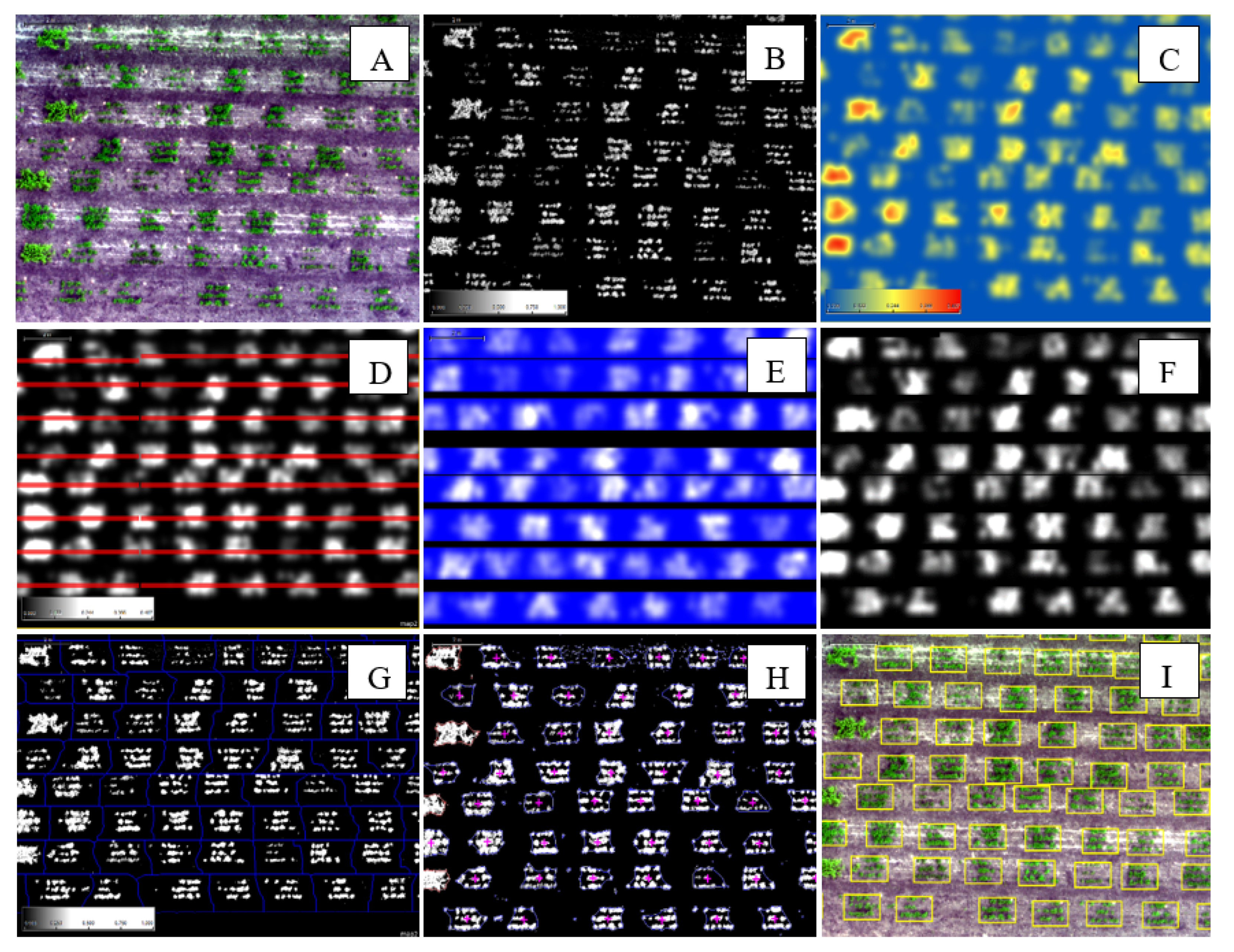
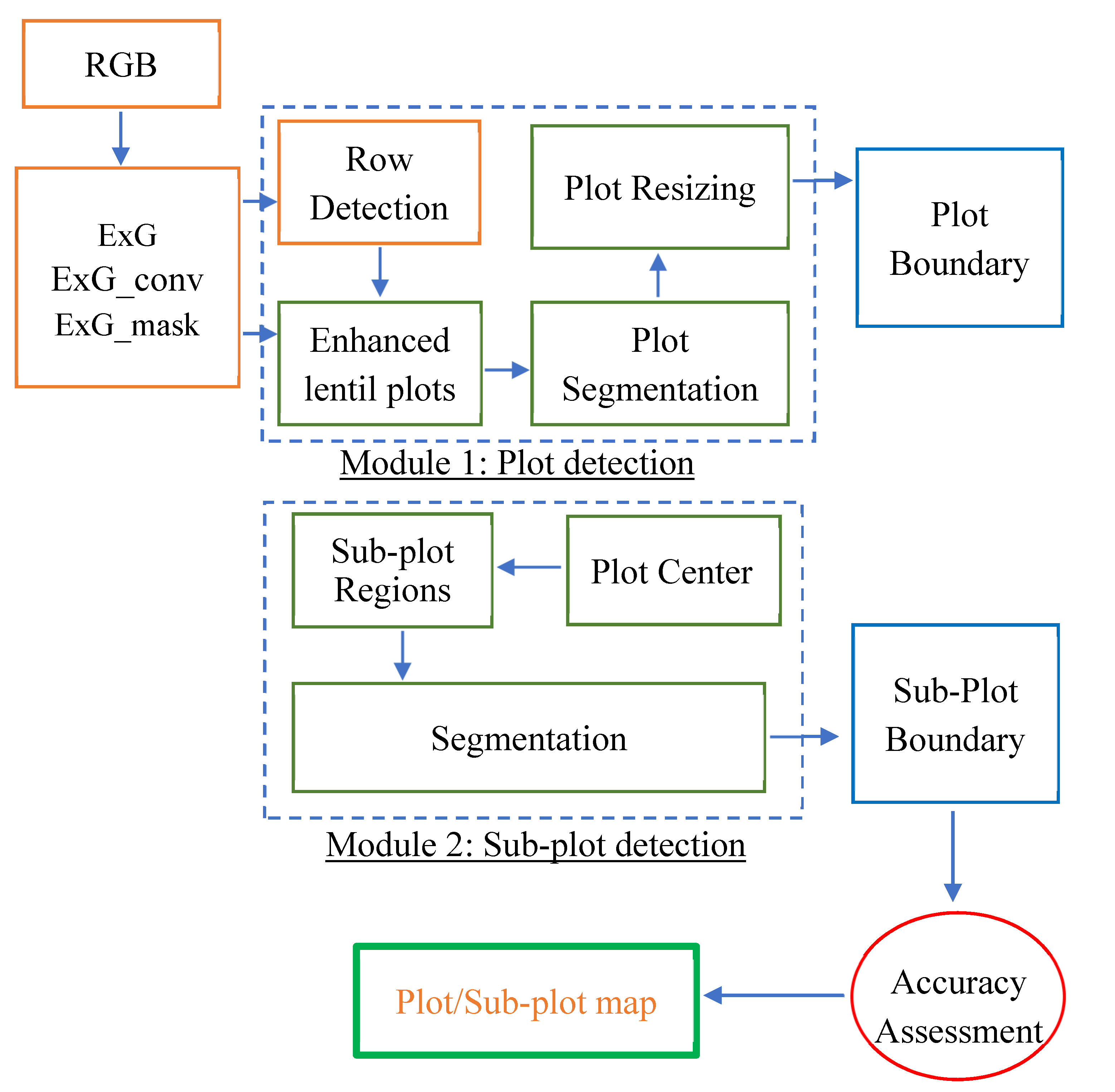
As lentils have low ground cover in early growth stages, the band math involves vegetation index calculation and image filter highlighting lentil plots. In this study, Excess Green Index (ExG) was calculated following equation [17]:

ExG = 2 × R_g − R_r − R_b

(1)

where R_g, R_r, and R_b are the reflectance values of green, red, and blue image bands, respectively.

RGB imagery (Figure 3A) is used to generate the ExG map (Figure 3B). Convolution filter (Gaussian) in window sizes range from 5 × 5 to 50 × 50 with the accumulative step of 5 × 5 pixels was conducted in a loop on ExG map. The output of the ExG convolution filter map (hereafter ExG_convo) is a raster layer map, as in Figure 3C. A greenness area mask (ExG_mask) was also created using a multi-thresholding algorithm on ExG, with a threshold value greater than 0 (ExG > 0). Map rotation was conducted (−1.45°) to align the crop rows horizontally and to facilitate the next steps.

2.5. Plot Detection

Four major steps were used to extract lentil plot boundary: (1) row detection, (2) plot enhancement, (3) plot segmentation, and (4) plot resizing.

In row detection, the ExG_convo image was used as an input. The major purpose of this step was to separate plots that have canopy overlapping from plots from one row to plots in the adjacent row. Chessboard segmentation and multiple object difference conditions-based fusion algorithm (Y center parameter = 0) were used to form horizontal row features. A local maxima algorithm with a searching range of 25 pixels was applied to locate row centers (Figure 3D). The algorithm located the object with the highest ExG_convo mean value within a certain searching distance. Once row centers were detected, pixel resizing (buffering) was used to form row boundaries to separate all lentil rows. The output was saved in a binary raster layer (row_mask; row = 1, row gab = 0, Figure 3E).

To enhance the lentil plot, band math of ExG_convo x row_mask was computed to mask out the gaps between rows. In the resultant map, all plots were highlighted on the ExG convolution map while all gaps between rows were defined (ExG_enhanced, Figure 3F). A watershed segmentation algorithm was then executed on ExG_enhanced (Figure 3G) with an object size parameter of 800 pixels. Watershed segmentation allows one to separate objects that are close together or where their edges touch. Pixel-based object resizing was applied with the following parameters.

The outcome of this process is depicted in Figure 3H. Centers of the object were then extracted and buffered into rectangular shapes, forming plot boundaries (Figure 3I).

In each plot, three sub-plots were aligned in rows (Figure 3A). The main purpose of this step was to separate the three rows in each plot. From the plot boundary map, a middle line was created from the plot center derived from the previous section (Figure 4A). Pixel resizing to the top and bottom was executed separately to form a unique region (Figure 4B). Multi-threshold and watershed segmentation algorithms were again used to classify the region’s objects into canopy and ground. In the canopy class, objects in top or bottom classes shared borders with the middle line and were re-classified into the middle class. Thus, the object relationship was considered to classify objects (Figure 4C). This process was applied to all plots. Pixel resizing was also used to refine the object, and the final sub-plot boundary is depicted in Figure 4D.

2.6. Accuracy Assessment

The plot and sub-plot extractions evaluation included quantifying the number of plots that were detected correctly and point-based accuracy assessment at the sub-plot level. At the sub-plot level, the confusion matrix was constructed to assess the accuracy of the classification result. There were 35 random plots selected for sub-plot accuracy assessment (AC) purposes. In the plots chosen, sub-plots were digitized and assigned manually to top, middle, and bottom classes. Additionally, 100 random points were generated within each plot. Information on classification and ground-truth was then collected on 3500 data points for the whole study area. A confusion matrix was constructed and calculated using a tool in ArcGIS Pro 2.4. The accuracy assessment indices include overall accuracy (OA), producer accuracy (PA), user accuracy (UA), and Kappa coefficient (K) [18].

3. Results and Discussion

3.1. Plot Boundary Map

A precise plot boundary map for all the plots (972) was generated, given the distance between plots and the ground cover inconsistencies. The precision of the plot boundary map generated was examined based on visual assessment. The plot boundary map of the entire field experiment is presented in Figure 5A, with a magnified sub-set (red box) showing irregularities in plot alignment and the output plot boundary map in detail.

As the input image was acquired during the mid-growing season, the ground cover percentage of most plots was at its peak. This facilitated the plot location through watershed segmentation. The segmentation algorithm presented here may need to be improved further to consider other issues relating to ground cover, especially for sub-plot segmentation. Images from the different growing stages are required to enhance the capability of the workflow, especially for sub-plot canopy overlap. In later stages of crop growth, where canopy overlapping is high, plot/sub-plot segmentation is particularly challenging [16]. However, as demonstrated in the sub-plot extraction, we believe our methodology can solve this issue.

Row detection using the local maxima algorithm (before plot detection) was critical to separate merging plots between rows. All lentil plots were highlighted by using a convolution filter in a loop (~10×, kernel sizes of 5 × 5 to 50 × 50) on a vegetation index (ExG), which facilitated the watershed segmentation process. Additionally, the pixel resizing algorithm with surface tension parameters (

Table 1. Pixel resizing parameters for lentil plot locating.

Mode	Pixel Constraint	Surface Tension Parameter
Shrink	ExG_enhanced < 0	Reference	object
		Operation	<=
		Value	0.55
		Box size X and Y	11
		Min. object size	2000

) allows us to detect the plot center precisely, and it was particularly useful in assigning the middle sub-plot (row).

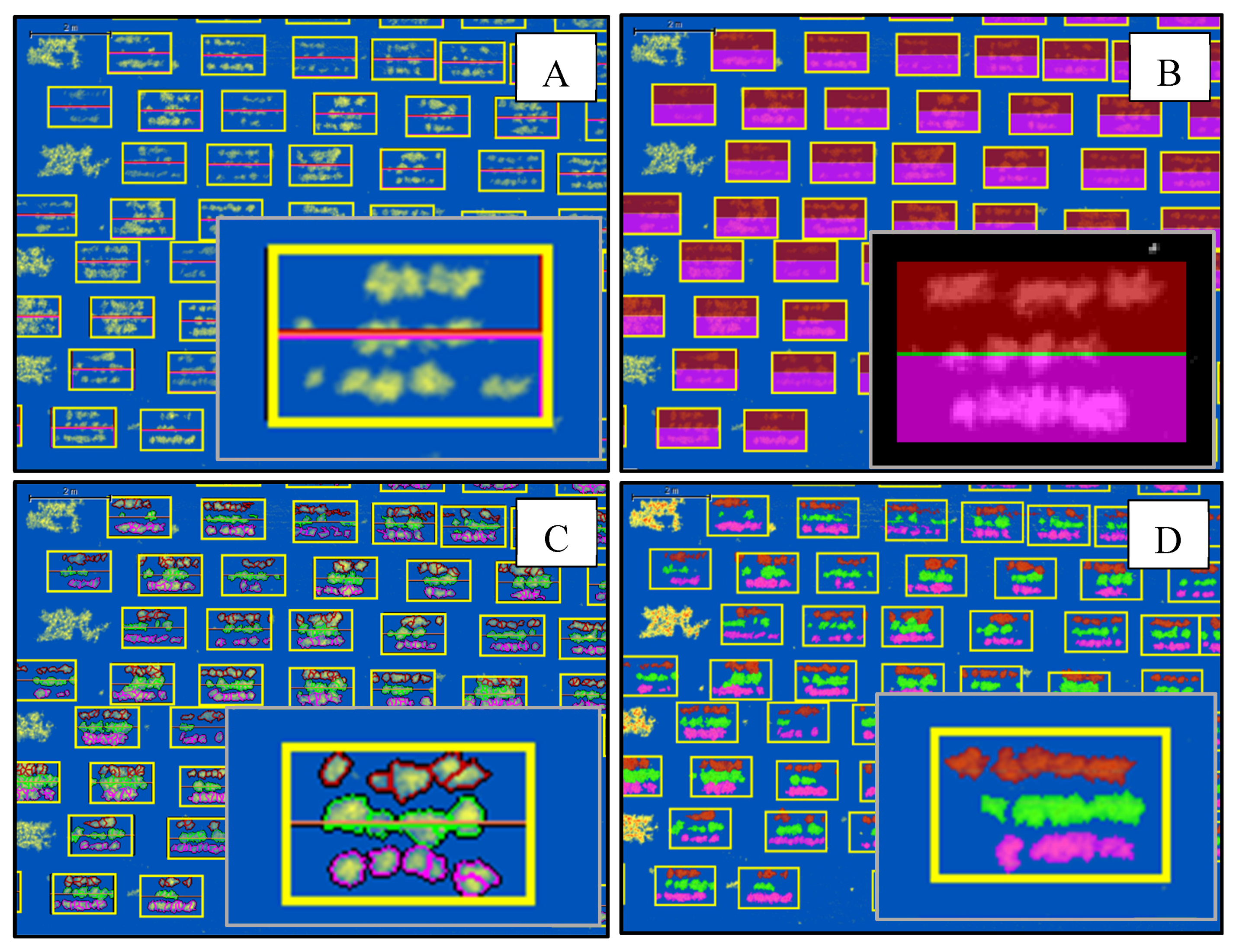
3.2. Sub-Plot Boundary Map

All the sub-plots (2916) were successfully extracted using a watershed segmentation algorithm and feature relation on each plot. The output map is presented in Figure 5B, with a magnified subset (red box) showing individual rows separated by color. It is important to note that rows within the plot were separated even in high plant covers where rows are merging, and individual rows were indistinct. The watershed segmentation algorithm was key to allowing this row separation. Within a sub-plot, the lentil blob can be approximately separated, as illustrated in Figure 5C, and the sub-plots were named using relative position inside plots, which are top, middle, and bottom. This information can be linked to field data, and information from plots, such as plot ID, can be transferred into a sub-plot as well.

3.3. Accuracy Assessment

Overall, the accuracy of the proposed methodology for plot and sub-plot extraction is high. The user and producer accuracies were greater than 85% across all sub-plot classes (

Table 2. Point-based accuracy assessment of sub-plot classification (three classes) error matrix using ground truth data (N = 3489) across lentil trials. Kappa value: 0.85; overall accuracy: 92%.

		Reference Data
	Classes	Top	Middle	Bottom	Ground	Total	User’s Accuracy
Classification	Top	345	0	0	46	391	0.88
	Middle	0	350	0	62	412	0.85
	Bottom	7	0	354	43	404	0.88
	Ground	45	29	53	2155	2282	0.94
	Total	397	379	407	2306	3489
	Producer’s Accuracy	0.87	0.92	0.87	0.93

). The corrected classified percentage was 92%, and the kappa coefficient (ranges from 0 to 1), measuring the agreement between the classified image and the reference image, is 0.85. The accuracy assessment suggests a strong agreement between the sub-plots generated by the workflow (classification) and the sub-plot digitized manually (ground truth data).

4. Conclusions

The workflow produced precise boundary maps for plots and sub-plots of the lentil breeding populations. Our methodology addressed some common issues such as plot alignment and overlapping canopies in the field experiments. In breeding studies, sub-plot measurements are important to attain greater precision in phenotypic data that can be linked back to genomic information. In continuation of this study, we extracted sub-plot level lentil flower number, plant height, and canopy volume over a growing season with greater precision than the plot-level measurements (data not shown).

The current workflow is considered semi-automatic as parameters such as map rotation, pixel resizing, or searching distance in the local maxima algorithm may need to be updated when the field conditions change. The ability to extract phenometric information at the sub-plot level provides opportunities to improve the precision of image-based phenotypic measurements at field-scale.

References

1. Liu, H.; Zhang, J.; Pan, Y.; Shuai, G.; Zhu, X.; Zhu, S. An Efficient Approach Based on UAV Orthographic Imagery to Map Paddy with Support of Field-Level Canopy Height from Point Cloud Data. IEEE J. Sel. Top. Appl. Earth Obs. Remote Sens. 2018, 11, 2034–2046. [Google Scholar] [CrossRef]
2. Niu, Y.; Zhang, L.; Zhang, H.; Han, W.; Peng, X. Estimating Above-Ground Biomass of Maize Using Features Derived from UAV-Based RGB Imagery. Remote Sens. 2019, 11, 1261. [Google Scholar] [CrossRef] [Green Version]
3. Makanza, R.; Zaman-Allah, M.; Cairns, J.E.; Magorokosho, C.; Tarekegne, A.; Olsen, M.; Prasanna, B.M. High-Throughput Phenotyping of Canopy Cover and Senescence in Maize Field Trials Using Aerial Digital Canopy Imaging. Remote Sens. 2018, 10, 330. [Google Scholar] [CrossRef] [PubMed] [Green Version]
4. Ubukawa, T.; De Sherbinin, A.; Onsrud, H.; Nelson, A.; Payne, K.; Cottray, O.; Maron, M. A Review of Roads Data Development Methodologies. Data Sci. J. 2014, 13, 45–66. [Google Scholar] [CrossRef]
5. Drover, D.; Nederend, J.; Reiche, B.; Deen, B.; Lee, L.; Taylor, G.W. The Guelph plot analyzer: Semi-automatic extraction of small-plot research data from aerial imagery. In Proceedings of the 14th International Conference on Precision Agriculture, Montreal, QC, Canada, 24–26 June 2018. [Google Scholar]
6. Haghighattalab, A.; Pérez, L.G.; Mondal, S.; Singh, D.; Schinstock, D.; Rutkoski, J.; Ortiz-Monasterio, I.; Singh, R.P.; Goodin, D.; Poland, J. Application of unmanned aerial systems for high throughput phenotyping of large wheat breeding nurseries. Plant Method. 2016, 12, 1–15. [Google Scholar] [CrossRef] [PubMed] [Green Version]
7. Anderson, S.L.; Murray, S.C.; Malambo, L.; Ratcliff, C.; Popescu, S.; Cope, D.; Chang, A.; Jung, J.; Thomasson, J.A. Prediction of Maize Grain Yield before Maturity Using Improved Temporal Height Estimates of Unmanned Aerial Systems. Plant Phenom. J. 2019, 2, 1–15. [Google Scholar] [CrossRef] [Green Version]
8. Csillik, O.; Cherbini, J.; Johnson, R.; Lyons, A.; Kelly, M. Identification of Citrus Trees from Unmanned Aerial Vehicle Imagery Using Convolutional Neural Networks. Drones 2018, 2, 39. [Google Scholar] [CrossRef] [Green Version]
9. Li, W.; Fu, H.; Yu, L.; Cracknell, A. Deep Learning Based Oil Palm Tree Detection and Counting for High-Resolution Remote Sensing Images. Remote Sens. 2016, 9, 22. [Google Scholar] [CrossRef] [Green Version]
10. Mubin, N.A.; Nadarajoo, E.; Shafri, H.Z.M.; Hamedianfar, A. Young and mature oil palm tree detection and counting using convolutional neural network deep learning method. Int. J. Remote Sens. 2019, 40, 7500–7515. [Google Scholar] [CrossRef]
11. Ampatzidis, Y.; Partel, V. UAV-Based High Throughput Phenotyping in Citrus Utilizing Multispectral Imaging and Artificial Intelligence. Remote Sens. 2019, 11, 410. [Google Scholar] [CrossRef] [Green Version]
12. Fareed, N.; Rehman, K. Integration of Remote Sensing and GIS to Extract Plantation Rows from A Drone-Based Image Point Cloud Digital Surface Model. ISPRS Int. J. Geo-Inf. 2020, 9, 151. [Google Scholar] [CrossRef] [Green Version]
13. Hassanein, M.; Khedr, M.; El-Sheimy, N. Crop row detection procedure using low-cost UAV imagery system. Int. Arch. Photogramm. Remote Sens. Spat. Inf. Sci. 2019, XLII-2/W13, 349–356. [Google Scholar] [CrossRef] [Green Version]
14. Torres-Sánchez, J.; Lopez-Granados, F.; Peña-Barragan, J.M. An automatic object-based method for optimal thresholding in UAV images: Application for vegetation detection in herbaceous crops. Comput. Electron. Agric. 2015, 114, 43–52. [Google Scholar] [CrossRef]
15. Khan, Z.; Miklavcic, S.J. An Automatic Field Plot Extraction Method from Aerial Orthomosaic Images. Front. Plant Sci. 2019, 10, 683. [Google Scholar] [CrossRef] [PubMed]
16. Ahmed, I.; Eramian, M.; Ovsyannikov, I.; van der Kamp, W.; Nielsen, K.; Duddu, H.S.; Rumali, A.; Shirtliffe, S.; Bett, K. Automatic Detection and Segmentation of Lentil Crop Breeding Plots from Multi-Spectral Images Captured by UAV-Mounted Camera. In Proceedings of the 2019 IEEE Winter Conference on Applications of Computer Vision (WACV), Waikoloa Village, HI, USA, 7–11 January 2018; pp. 1673–1681. [Google Scholar] [CrossRef]
17. Woebbecke, D.M.; Meyer, G.E.; Von Bargen, K.; Mortensen, D.A. Color Indices for Weed Identification Under Various Soil, Residue, and Lighting Conditions. Trans. ASAE 1995, 38, 259–269. [Google Scholar] [CrossRef]
18. Congalton, R.G. A review of assessing the accuracy of classifications of remotely sensed data. Remote Sens. Environ. 1991, 37, 35–46. [Google Scholar] [CrossRef]
Figure 1. (A) The lentil breeding trial within field boundary (red) in RGB color. (B) Subset of the orthomosaic showing sample crop row, plot, and sub-plot. (C) Excess green vegetation index (ExG) map of the subset.
Remotesensing 13 04997 g001
Figure 2. The overall workflow for plot and sub-plot extraction from UAV color (RGB) imagery. ExG: Excess Green Index; ExG_mask: ExG > 0; ExG_conv: ExG enhanced using convolution filter; RGB: image in red, green, and blue composite.
Remotesensing 13 04997 g002
Figure 3. Example subsets illustrate plot extraction process. (A) RGB image of the plots. (B) ExG index. (C) ExG after convolution filter (ExG_convo). (D) Center row detection (in red). (E) Row mask (row_mask). (F) ExG_convo after mask out row gap to enhance lentil plot (ExG_enhanced). (G) Plot segmentation boundary (in blue line). (H) Plot boundary formation using pixel-based object resizing and plot center (purple point). (I) Final plot boundary 2.6. Sub-plot detection.
Remotesensing 13 04997 g003
Figure 4. Example to illustrate sub-plot extraction from plot boundary and ExG index. (A) Plot center and middle line. (B) Plot regions—middle, top, and bottom. (C) Watershed segmentation output. (D) Final sub-plot boundary map layer.
Remotesensing 13 04997 g004
Figure 5. The output maps of (A) plot boundary (yellow boxes). (B) Sub-plot map showing individual rows separated by color. (C) Vector maps (plot and sub-plot) of the whole experiment. The magnified regions are in the red boxes.
Remotesensing 13 04997 g005