Article

Non-Destructive Monitoring of Maize Nitrogen Concentration Using a Hyperspectral LiDAR: An Evaluation from Leaf-Level to Plant-Level

1
The State Key Laboratory of Remote Sensing Science, Aerospace Information Research Institute, Chinese Academy of Sciences, Beijing 100101, China
2
University of Chinese Academy of Sciences, Beijing 100049, China
3
College of Land Science and Technology, China Agricultural University, Beijing 100193, China
4
State Environment Protection Key Laboratory of Satellite Remote Sensing, Aerospace Information Research Institute, Chinese Academy of Sciences, Beijing 100094, China
*
Author to whom correspondence should be addressed.
Remote Sens. 2021, 13(24), 5025; https://doi.org/10.3390/rs13245025
Submission received: 27 October 2021 / Revised: 7 December 2021 / Accepted: 8 December 2021 / Published: 10 December 2021

Abstract

:
Advanced remote sensing techniques for estimating crop nitrogen (N) are crucial for optimizing N fertilizer management. Hyperspectral LiDAR (HSL) data, with both spectral and spatial information of the targets, can extract more plant properties than traditional LiDAR and hyperspectral imaging systems. In this study, we tested the ability of HSL in terms of estimating maize N concentration at the leaf-level by using spectral indices and partial least squares regression (PLSR) methods. Subsequently, the N estimation was scaled up to the plant-level based on HSL point clouds. Biomass, extracted with structural proxies, was utilized to exhibit its supplemental effect on N concentration. The results show that HSL has the ability to extract N concentrations at both the leaf-level and the canopy-level, and PLSR showed better performance (R2 > 0.6) than the single spectral index (R2 > 0.4). In comparison to the stem height and maximum canopy width, the plant height had the strongest ability (R2 = 0.88) to estimate biomass. Future research should utilize larger datasets to test the viability of using HSL to monitor the N concentration of crops, which is beneficial for precision agriculture.

Graphical Abstract

1. Introduction

Nitrogen (N) is a crucial element in agriculture, since N significantly affects the physiological processes of plants and, thus, affects their growth and yield [1,2]. Crops generally receive N through chemical fertilizers; N deficiency results in a decline in the quantity and quality of crop yield, while an oversupply of N could lead to plant disease and environmental damage [3,4]. Given the important role N plays in plant growth, improving the N-use efficiency (NUE) is helpful for agronomic and breeding research [5]. Thus, the dynamic monitoring of crop N helps optimize N fertilizer management.
The distribution of N within a plant canopy is spatially heterogeneous, since plant canopies are three-dimensional (3D) structures [6,7]. This vertical distribution pattern matches the available radiation along the plant height to achieve the maximum canopy photosynthesis [8], since about 75% of leaf nitrogen is involved in the plant photosynthesis process [2], and previous studies have shown that shaded leaves in the canopy bottom have lower N than upper leaves that are exposed to sunlight [9,10]. In addition, the N distribution is a dynamic process (instead of a static one), which is related to the growth stages and environmental conditions [1]. The plant N concentration is closely related to plant structural proxies, whereas the N concentration decreases with increases in the biomass [5,11,12,13], and is proportional to the leaf area index (LAI) [14]. Thus, understanding the N spatial distribution pattern, as well as the simultaneous extraction of both N content and plant structural parameters, are imperative for precise N estimations.
Destructive sampling methods, such as the Kjeldahl method [15], are time-consuming and labor intensive, although they have high accuracies. The optical remote sensing technique, based on the strong correlation between plant biochemical parameters and reflected spectral properties, has been widely used in N estimation in several fields of research [16,17,18,19]. However, the heterogeneous nature of N distributions affects the monitored reflectance spectra and, thus, the accuracy of N estimation [7,20,21]. Despite both the top view [6,7,22] and multi-angle observations [23,24] having been used for detecting the vertical properties of biochemical parameters, these indirect methods have limited effectiveness and still lack plant structural information. The structure from motion (SFM) method, building plant point clouds with multi-angle two-dimensional (2D) images, has been used to characterize plant three-dimensional (3D) biochemical properties [25]; however, its data-collection process is laborious, and the spectral information of the constructed point cloud was limited.
Light detection and ranging (LiDAR) actively emits laser pulses and records the backscattered intensity of the targets. This kind of active remote sensing technique has certain advantages in comparison to passive remote sensors. First, the data collection of LiDAR is independent of illumination conditions; therefore, it can operate both day and night, achieving continuous observation over a long period [26]. Second, LiDAR observation is less affected by viewing angles and background noise, since it records signals at a ‘hot-spot’ and its instantaneous field of view is relatively small [27,28]. Third, LiDAR can penetrate plant canopies; it has been widely used to extract plant structural parameters based on its recorded ranging information [29,30,31,32]. Despite traditional LiDAR systems having limited wavelength bands, previous studies have tested the possibility of using the LiDAR backscattered intensity for estimating plant biochemical properties. For example, Zhu et al. [33] characterized the 3D distribution of plant water using a LiDAR system employing an SWIR (1550 nm) laser. Eitel et al. [34] used a LiDAR employing a green laser (532 nm) to determine leaf chlorophyll levels, and Gaulton et al. [28] utilized a LiDAR with two wavelength bands (1063 nm and 1545 nm) to estimate vegetation moisture content. To further combine the advantages of spectral imaging and LiDAR, certain approaches have been developed. One involves the fusion of passive remote-sensing data and LiDAR data [35], where the acquisition of passive data still relies on lighting conditions and the 2D spectral imaging contains less spectral information regarding the canopy bottom [26]. The registration of multiple LiDAR point clouds with different wavelength bands is another approach [36,37], while point clouds obtained using several sensors have certain advantages.
The best way to generate point clouds with abundant spectral information is to develop LiDAR systems with different wavelength bands; therefore, the advantages of spectral imaging and LiDAR can be combined into a single system. Owing to the development of a supercontinuum laser source, which has a high power laser and covers a wide spectral range [38], several researchers have developed prototype hyperspectral LiDAR (HSL) systems [39,40,41,42]. HSL has the ability to simultaneously extract abundant spectral and ranging information, facilitating the generation of a spectral point cloud through data processes. As an active remote sensor, HSL has fewer complex confounding factors (e.g., lighting conditions, soil background, and the viewing angle), which significantly affect passive optical remote sensors. Despite the heterogeneous distribution of N within plant canopies, the estimation of N concentration in previous studies was conducted using 2D leaves rather than 3D plant structures [43,44,45]. Plant structural and biochemical parameters are the two main types of features of crops; however, previous studies did not simultaneously extract plant structural traits to explore the supplementary effect of structural parameters on biochemical properties.
The importance of estimating N in maize plants has been emphasized by previous studies [46,47,48]. Thus, we aim to (1) estimate maize N concentration from the leaf-level to the plant-level and (2) extract plant biomass based on structural proxies to better characterize the 3D properties of maize plants. This study attempts to explore whether HSL can be used as an effective tool in evaluating plant N status, which helps improve N fertilizer management and crop yield. With the development of HSL hardware, this technique can be used in both scientific research and practical agricultural applications.

2. Materials and Methods
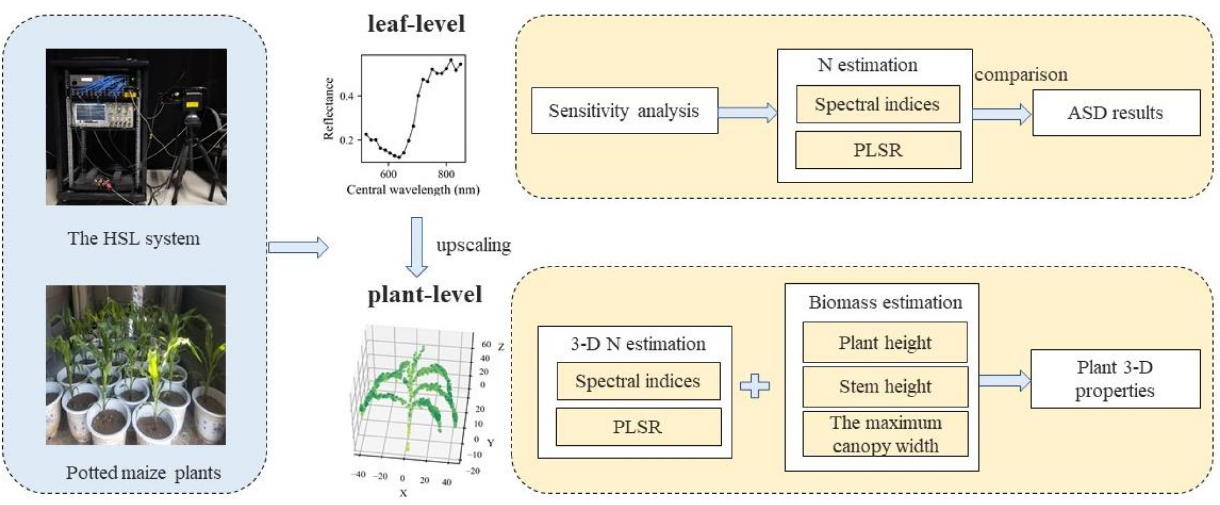
2.1. Overview

The workflow of this study is illustrated in Figure 1. Using a prototype HSL device developed by our research community [49], this study estimated the maize N concentration from the 2D leaf level to the 3D plant level.

2.2. Data Collection and Preparation

2.2.1. Maize Plants

Maize plants were cultivated at the National Experiment Station for Precision Agriculture in 2021. This site lies in Changping District, Beijing, China. Its mean annual temperature is about 13 °C and the mean annual rainfall is about 507.7 mm. Given the demand for the experiment, all maize seeds were planted in flowerpots for about 2 months. Potted maize plants—with heights ranging from 50 to 100 cm—were transported to the laboratory for data collection.

2.2.2. HSL Data Collection

The HSL system developed by our research community was used for the scanning of maize plants. The system consists of an SC laser source, ranging from 450 to 2400 nm; an optical receiver used to collect the backscattered intensity reflected by targets; and a signal acquisition system that can convert light signals to electrical signals. The maximum wavelength band of the HSL system was 32 bands, since the PMT array used to collect signals was only sensitive to wavelengths ranging from 300 to 920 nm. In this experiment, 20 wavelength bands—with their center wavelengths ranging from 523 to 833 nm—were used. Their spectral resolution was 16 or 17 nm.
Maize leaves (n = 60) were randomly selected from maize plants. They were pasted on a black background panel and subsequently used for HSL scanning at a distance of 5 m. Before the measurement of each leaf, a white reference panel at the same position was also scanned to normalize the backscattered intensity. During the scanning process, all lights in the laboratory were turned off, since HSL actively emits laser pulses and external illuminators could affect the scanning process.
In addition to 2D maize leaves, maize plants (n = 27) were also scanned using the HSL system. Potted maize plants were also placed 5 m in the front of the HSL system. Other settings were the same as those used for 2D maize leaves.

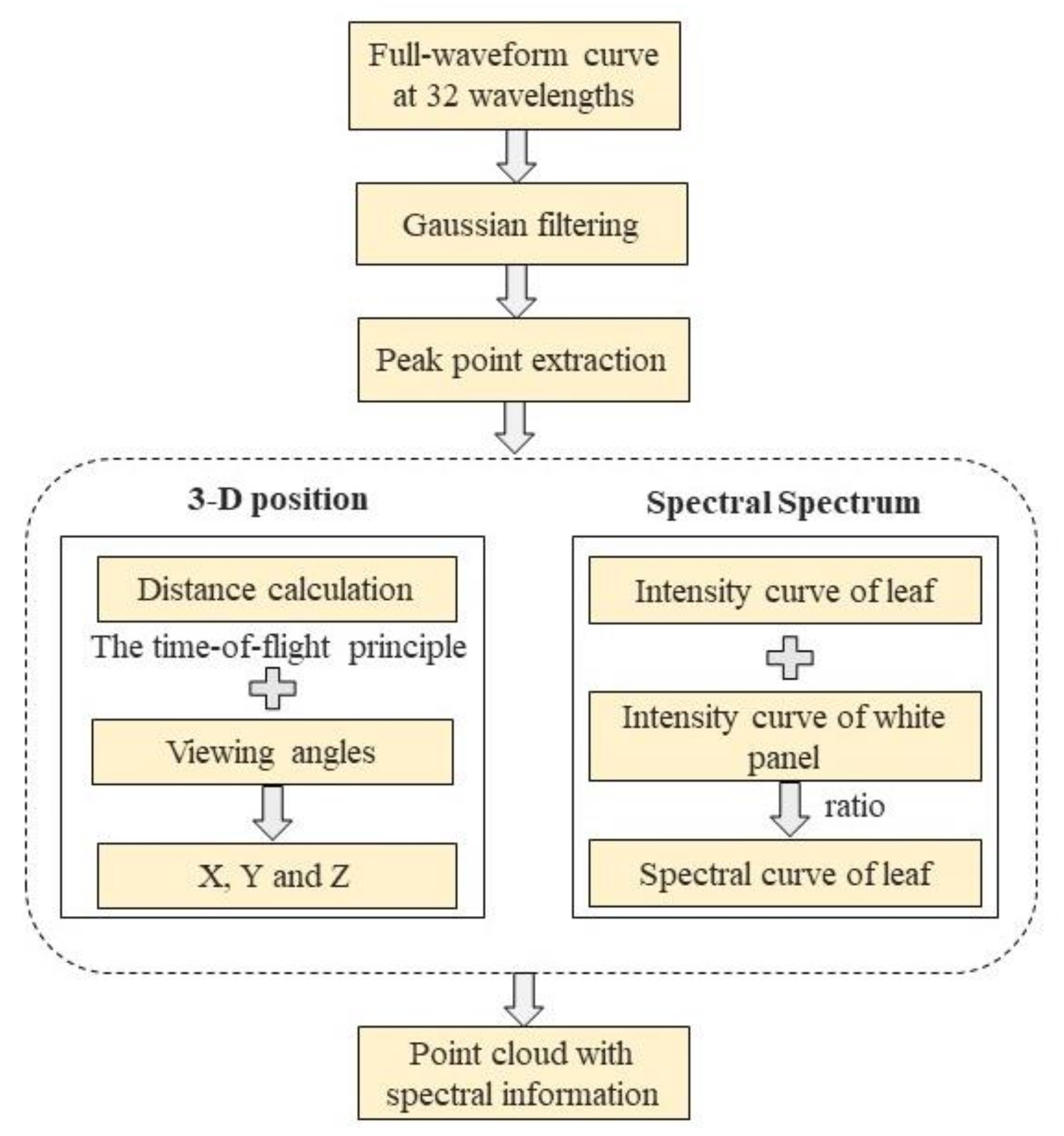
2.2.3. HSL Data Processing

The HSL full-waveform data were saved in the comma-separated values (.csv) format. To extract the spectral and structural information of targets, several steps were required for data processing, as shown in (Figure 2).
To remove the noise that appeared in the optical path and HSL hardware, Gaussian filtering was first applied to the full-waveform data. Based on the filtered data, the maximum returned intensity and flight time of the peak point were extracted, which were used for further calculating the 3D position and spectrum of each point. The distance between each target point and HSL was calculated using the time-of-flight principle, where the distance = (3 × 10⁸ m/s × the flight time)/2. Thus, the X, Y, and Z positions of each point could be obtained when coupled with the viewing angle and the trigonometric function. The reflectance of leaves can be derived by calculating the ratio of intensity between leaves and the reference panel. Through the above processing steps, point clouds with 20 wavelength bands were derived.

2.2.4. Passive Spectral Data Collection

A handheld spectroradiometer (Analytical Spectral Devices, Inc.—ASD, Boulder, CO, USA)—which measures the spectrum ranging from 400 to 2500 nm with a spectral resolution of 1 nm—was also used for the collection of spectral data at the 2D leaf-level. This passive remote sensor was widely used in various applications due to its high spectral accuracy [50,51,52]. Consistent with the measurement conditions of HSL, the spectral collection of maize leaves was conducted in a dark laboratory. To provide a light source for ASD, an illuminator was placed about 50 cm above the leaves. Twenty reflectance spectra were recorded and averaged for each leaf to increase the signal-to-noise ratio of recorded signals. Owing to the differences in the spectral resolution between HSL and ASD data, the ASD data with a higher spectral resolution was resampled according to the wavelength bands of HSL.

2.2.5. N Concentration Determination

Each 2D leaf was placed in a labeled plastic bag after spectral collection. For 3D maize plants, the leaves of their canopy were pulled off and placed in bags after HSL and ASD data collection. Maize samples were over-dried, at a temperature of 105 °C, until their weight was constant, and the N concentration of both 2D leaves and 3D canopies were determined by the Kjeldahl method.

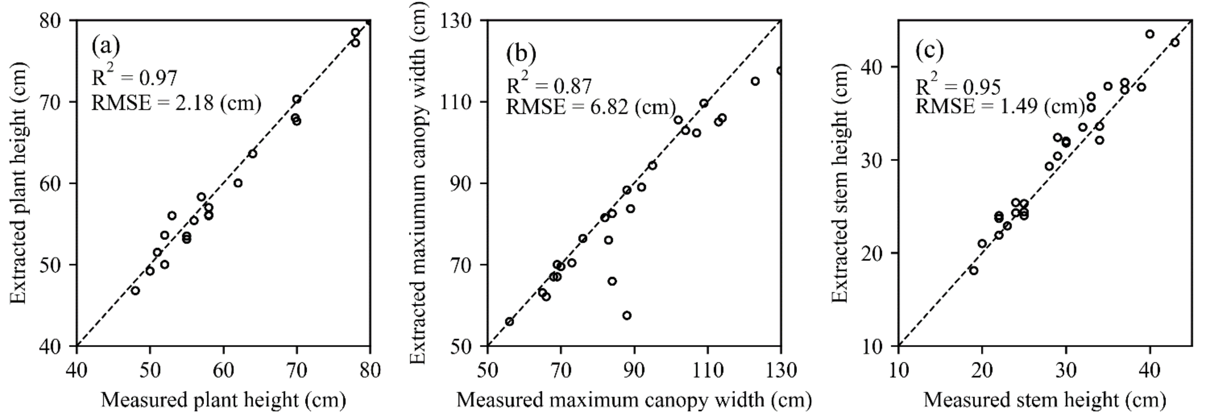
2.2.6. Structural Parameter Measurement

Several structural parameters (plant height, stem height, the maximum canopy width, and biomass) of 3D maize plants were measured manually. The plant height was defined as the vertical distance between the highest point of the maize and the soil, the stem height represented the distance between the top point of the stem and the soil, and the maximum canopy width was defined as the maximum width of the maize canopy. The actual values of the above three variables were manually measured, with the position of the maize plants maintained constant. The biomass was defined as the dry mass of the maize canopy, which was measured after oven drying and weighing the samples.

2.3. Leaf-Level Analysis

Based on the simulation results from the PROSPECT-5 model, the sensitivity analysis could successfully identify the contribution of the biochemical parameters to the reflectance. The input structural parameter (N), chlorophyll content, carotenoids, and leaf mass per area (LMA) were set to vary in the range of 1.0–3.5, 0–100 μ g / cm 2 , 0–30 μ g / cm 2 , and 0.0008–0.0331 g/ cm 2 , respectively. The N estimation process at the leaf-level was conducted by using both single spectral indices and PLSRs with ten selected indices as inputs; thus, the correlation between measured and estimated values can be derived. The estimation result was subsequently compared with the passive remote sensing data collected by ASD, since its collected spectrum had been widely regarded as the standard reflectance. The ASD data were resampled according to the HSL wavelength bands.
Partial least squares regression (PLSR) is a linear nonparametric estimating method that applies linear transformation and has been recognized as a standard method for retrieving biochemical parameters [53]. PLSR constructs a linear multivariate between reflectance and a target trait, making it suitable for small datasets, as shown in Equation (1):
Y = β X + ε
where X and Y represent the mean-centered matrix of the independent and dependent variables, respectively. β is the regression coefficient, and ε represents the residuals matrix. Owing to the effectiveness of PLSR, it has been widely used for plant N estimation [17,54].
Spectral indices are the most popular estimation approaches, and are designed to be sensitive to target vegetation properties, remaining unaffected by other disturbances. Ten spectral indices (Table 1) in the ratio and normalized format were chosen for this study. When calculating spectral indices, the wavelength bands of the collected dataset closest to the bands required by the formulas were used.

2.4. Plant-Level Analysis

Based on the analysis of 2D maize leaves, N estimation was then upscaled and conducted at the 3D canopy level. Eliminating the incident angle effect is a prerequisite for using spectral information at different points. The ratio and normalized spectral indices have been confirmed to largely eliminate the incident angle effect that occurs in HSL point clouds [63], as the confounding factors of different wavelength bands were similar along the optical path [64]. Thus, the PLSR method was applied with ten selected spectral indices, instead of the spectrum, as inputs. Considering the supplementary effect of biomass to N concentration [65,66], the biomass of the maize canopy was also extracted using three structural proxies (plant height, stem height, and maximum canopy width). These three structural proxies of the constructed maize point cloud were obtained manually using the CloudCompare software.
The fitness between the measured and estimated values was evaluated by the coefficient of determination (R2) and root mean square error (RMSE). The statistical analysis process was conducted in a Python environment.

3. Results

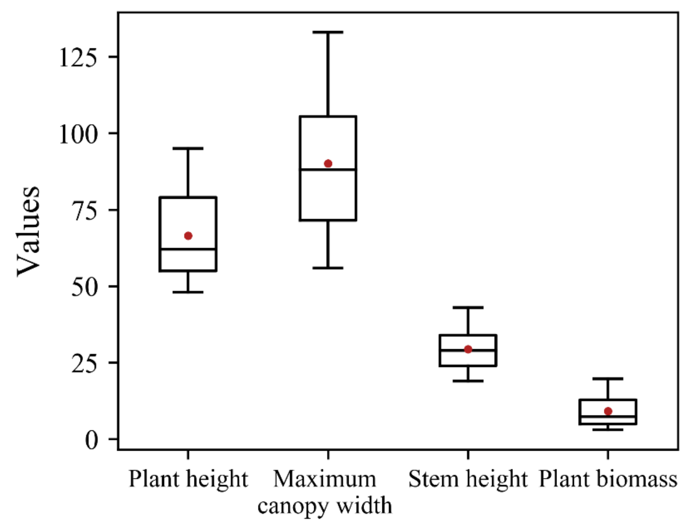
3.1. Distribution of the Measured Data

3.1.1. N Concentration and Structural Properties

The statistical values of the N concentration determined by the Kjeldahl method are given in Table 2. The minimum, maximum, and mean values of N for the maize leaves differed from those for maize canopies. The minimum values of leaf and canopy N were 0.54% and 0.30%, respectively; the maximum values of these two datasets were 0.80% and 0.50%, respectively. This indicates that the measured leaf N had a wider variation range than the canopy. The mean value of leaf N was 0.65%, while the value of canopy N was only 0.39%.
The measured structural proxies are illustrated in the form of box plots (Figure 3). All measured structural values were relatively small, since the crops were planted in flowerpots instead of in the field. The biomass of maize plants varied between 3 and 20 g, and the height varied between 48 and 95 cm, implying that the experimental maize plants had a large gap in growth status.

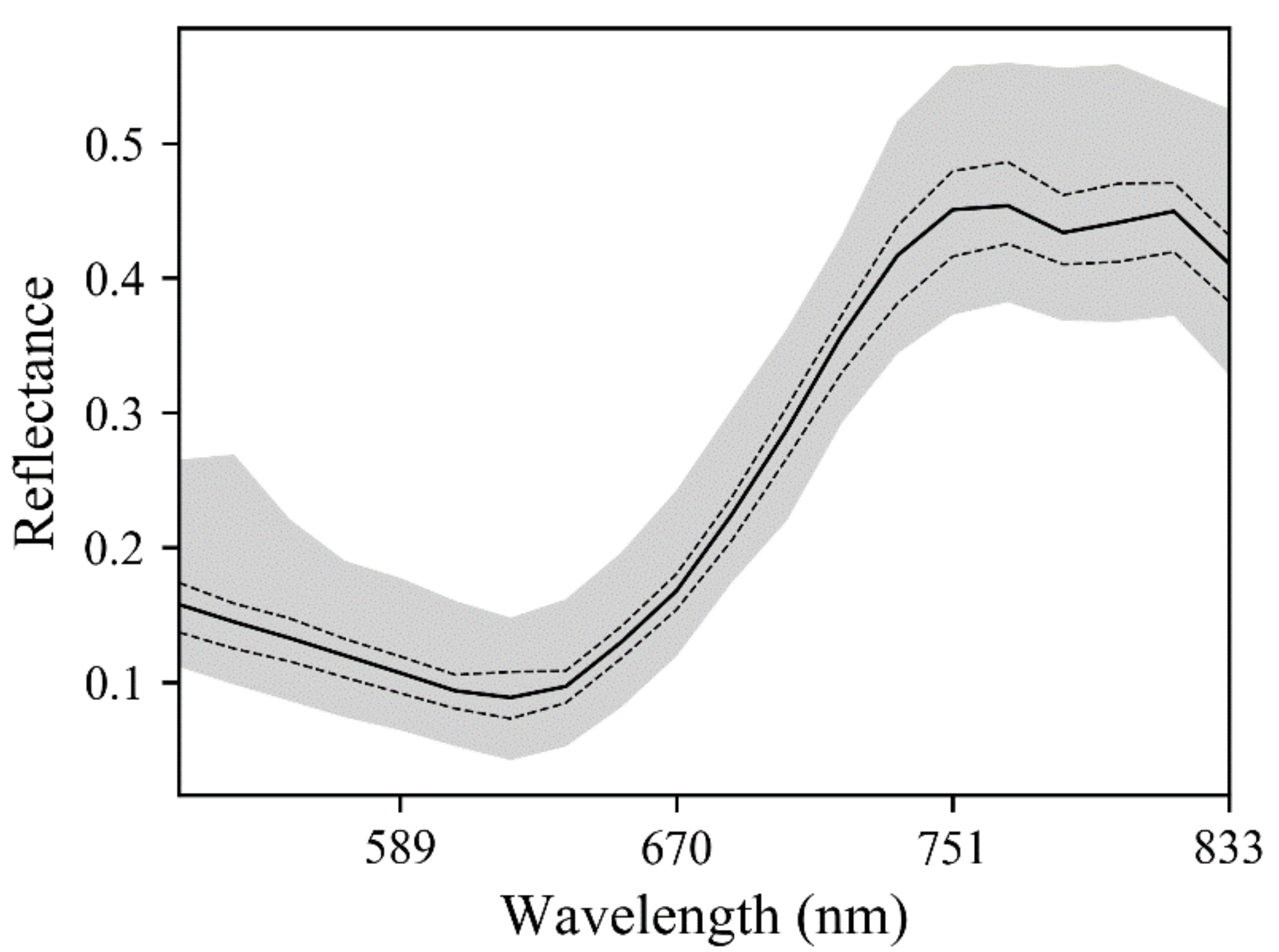
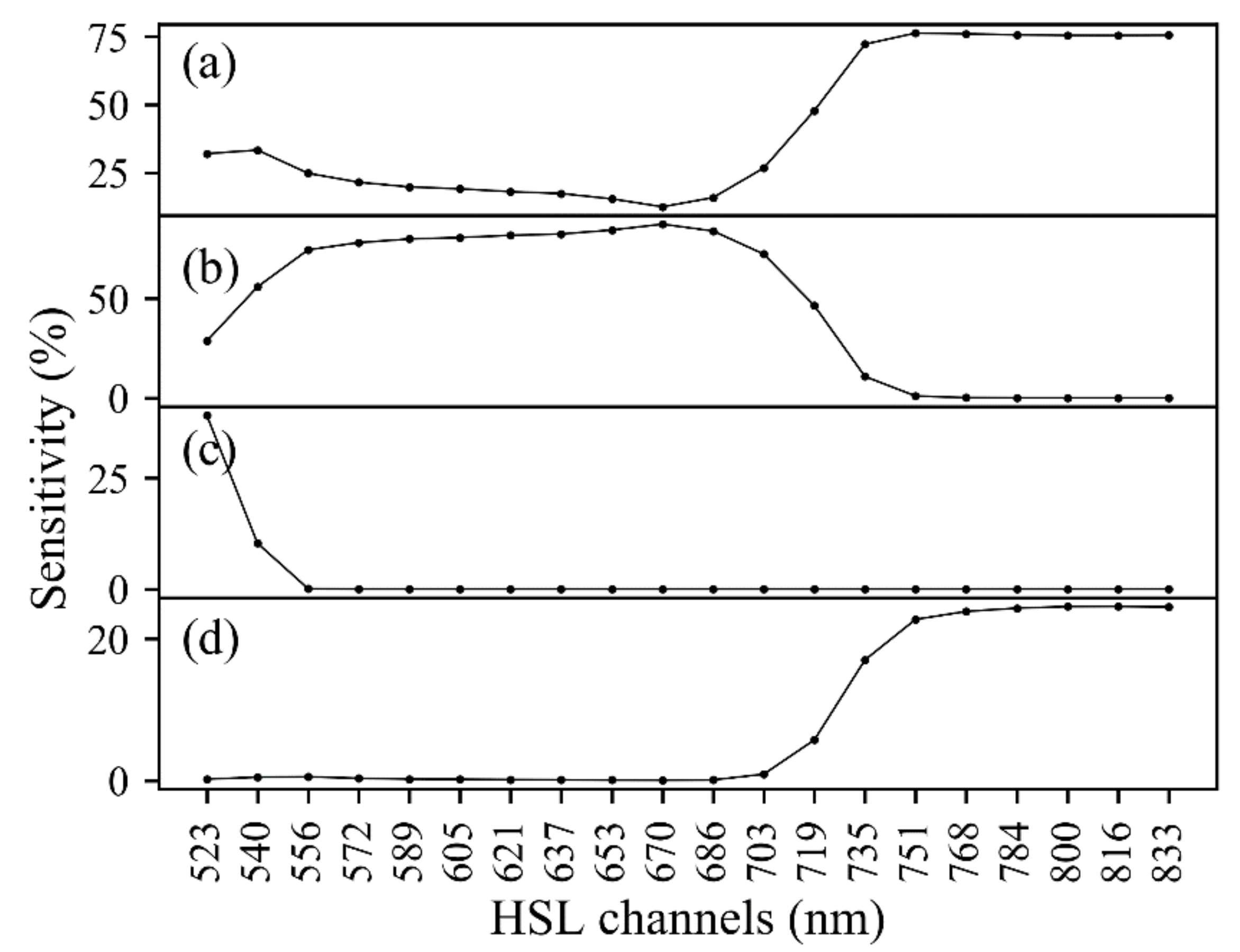
3.1.2. Spectrum of HSL

Spectra collected with 2D maize leaves were used to analyze the reflectance characteristics of HSL data. The medium value, variation range, and the first and third quartile of each wavelength band are shown (Figure 4). The reflectance curve—consisting of 20 HSL wavelength bands—was relatively smooth, with the inner wavelength bands, had a higher signal-to-noise ratio. There was an increasing trend in the red edge region (670–760 nm), which was known to be sensitive to multiple plant properties (e.g., chlorophyll, nitrogen, and carotenoids).
A sensitivity analysis was performed to analyze the contribution of plant biochemical parameters to the variation of the HSL reflectance spectrum (Figure 5). Although the central wavelength and spectral resolution of HSL data differed from that of commercial systems, the 20 HSL wavelength bands were sensitive to target traits. The variation in the plant structure accounted for more than 70% of the variation of reflectance above 735 nm. The variation in chlorophyll contributed more than 50% to the reflectance within 523–719 nm. Given the close relationship between N and chlorophyll, it can be inferred that the selected HSL wavelength bands could help estimate maize N concentration.

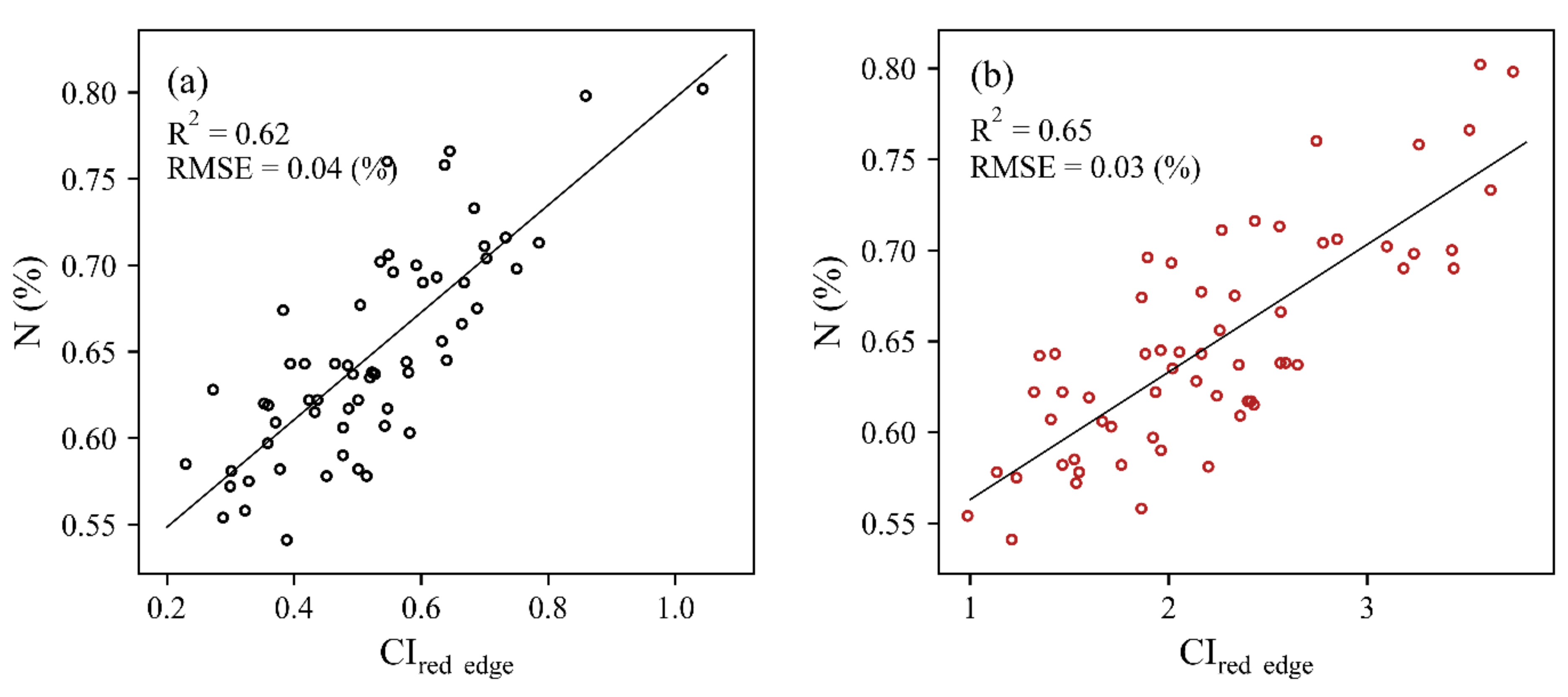
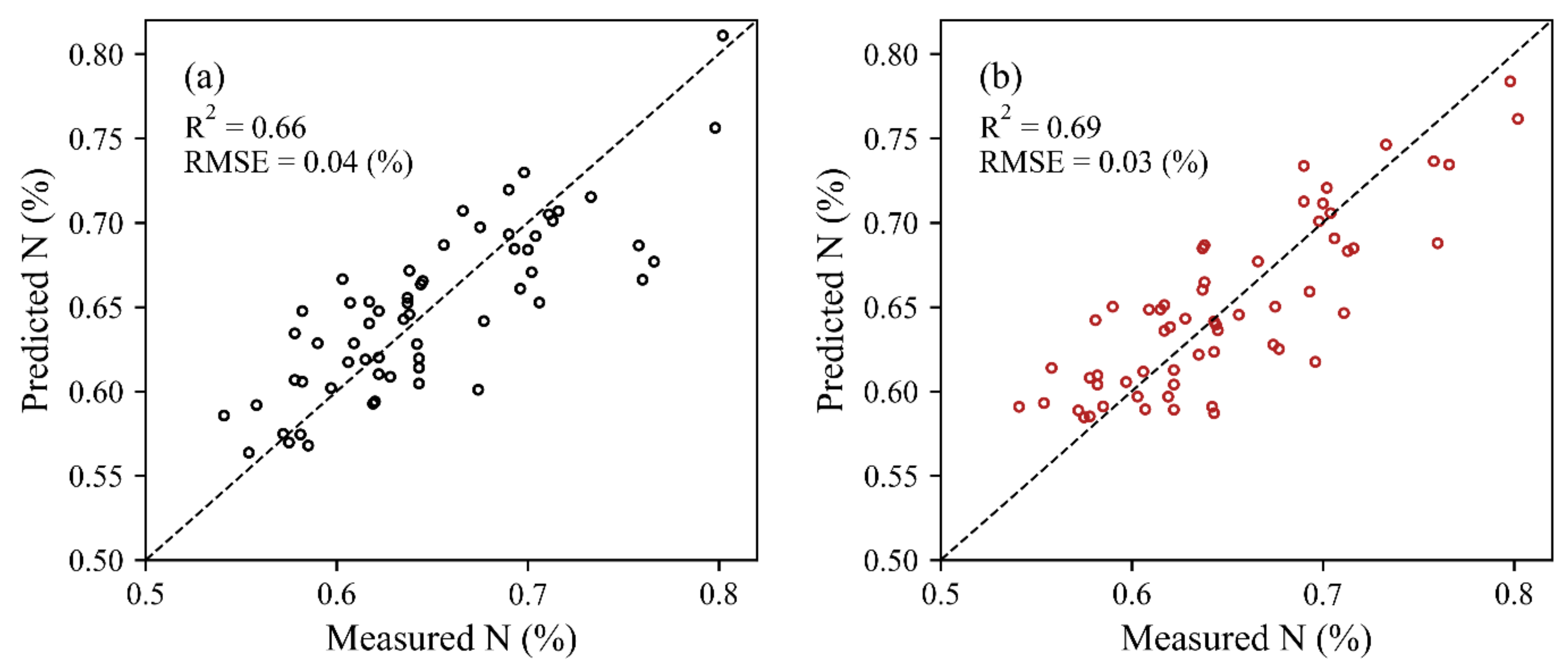
3.2. Estimation of the N Concentration at the Leaf-Level

Before characterizing the 3D N concentration of maize, the ability of HSL for N estimation was first tested using 2D maize leaves. The dataset collected for maize leaves was less affected by the confounding factors, such as the incident angle and edge effect, providing the basis for N estimation at the plant-level.
The selected ratio and normalized spectral indices exhibited distinct differences in terms of N estimation (Table 3). All spectral indices had a positive correlation with N concentration, with the highest accuracy (R2 = 0.62 for HSL and 0.65 for ASD) being obtained using the CIred edge index. The data pairs of N concentration and CIred edge values are illustrated in Figure 6.
With ten spectral indices as inputs, the PLSR model exhibited a good ability to estimate the N concentration, since the data points were closer to the 1:1 line (Figure 7). The fitness between the measured and estimated values of PLSR was better than that obtained using spectral indices, with the estimation accuracy of ASD (R2 = 0.70, RMSE = 0.03%) being higher than that of HSL (R2 = 0.66, RMSE = 0.04%).

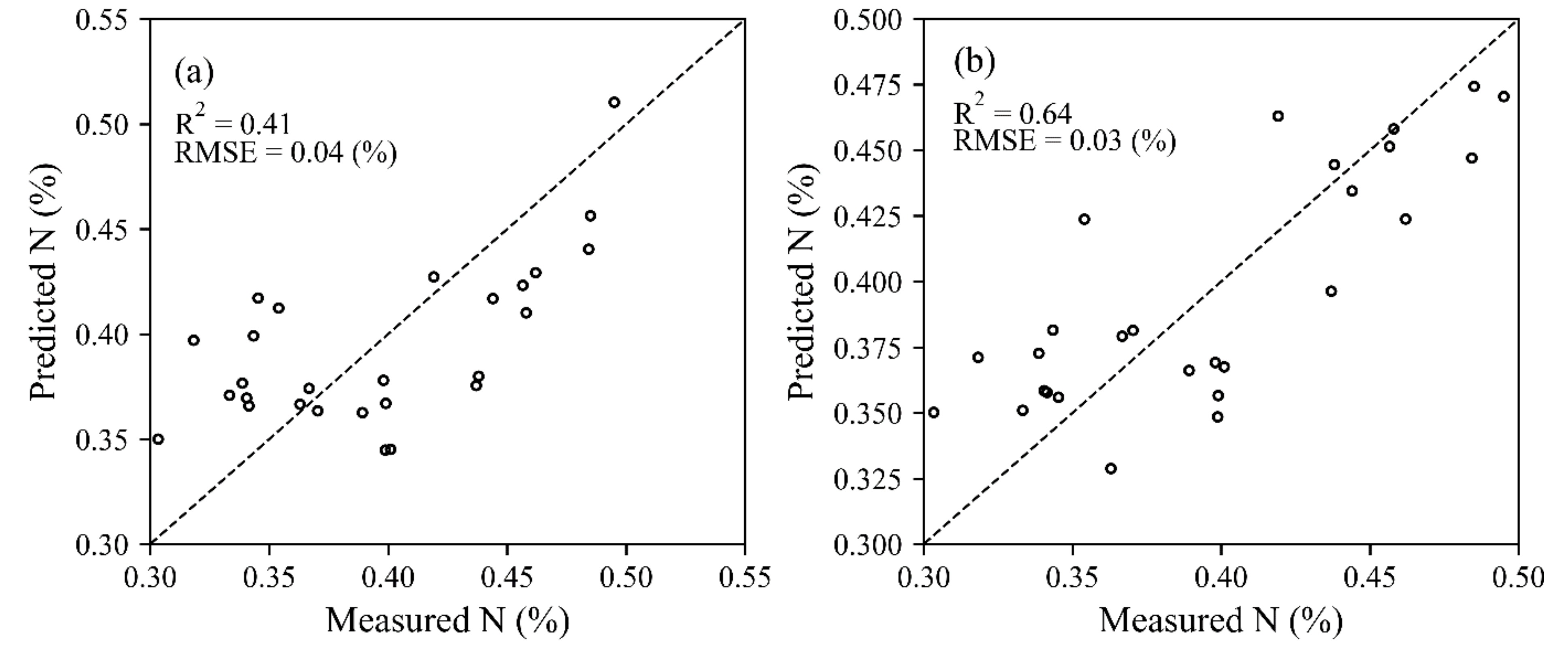
3.3. Estimation of the N Concentration at the Plant-Level

The 3D point cloud for maize plants, containing both spectral and structural information, was generated from HSL full-waveform data. The structure of one maize plant is clearly illustrated in Figure 8a; both its stem and leaves were successfully scanned by HSL. The density of the data points was relatively sparse owing to the fact that the scanning step of HSL was set to be large in this experiment. Based on the analysis at the 2D leaf-level, the capacity of HSL for monitoring the 3D N concentration was further explored. Considering that the CIred edge calculated using the HSL wavelength bands had the strongest correlation with N concentration, the estimation result of the PLSR method was compared with that of CIred edge (Figure 9). PLSR with spectral indices as inputs exhibited better performance (R2 = 0.64, RMSE = 0.03%) than the best-performing index (R2 = 0.41, RMSE = 0.04%) owing to the abundant spectral information contained in all selected indices and the effectiveness of the PLSR method. To show the N concentration distribution in 3D space, the N concentration of an entire maize plant—based on the constructed PLSR method—is shown in Figure 8b.

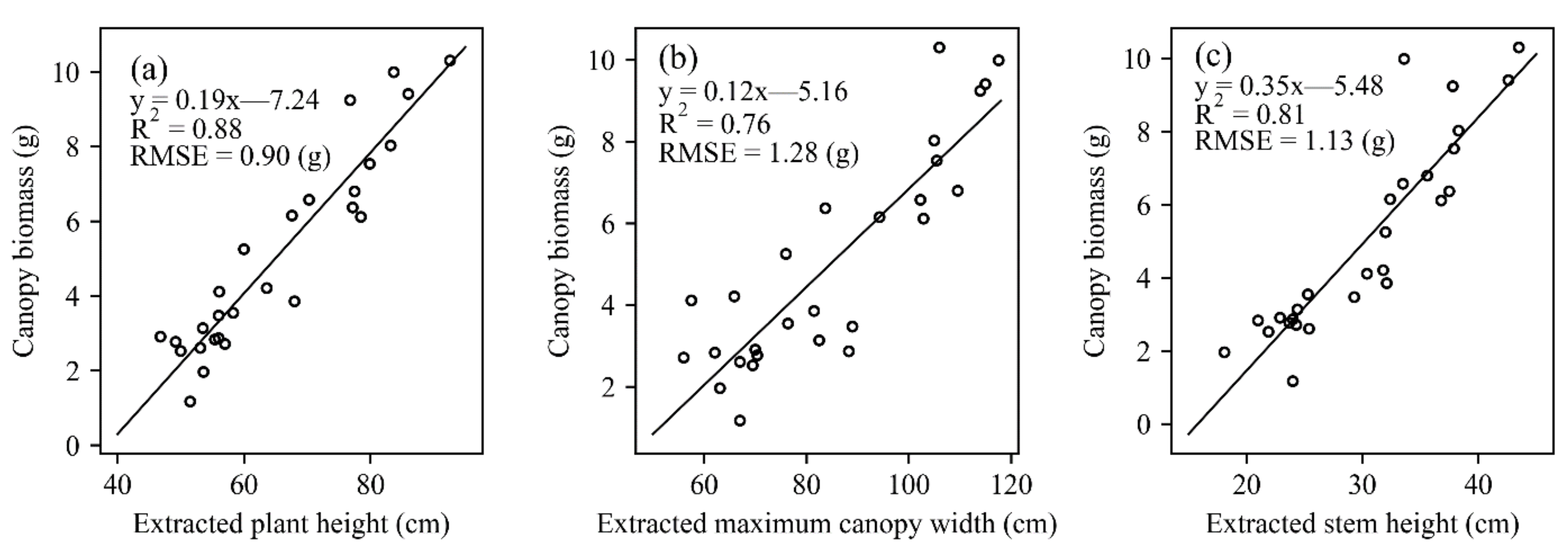
3.4. Estimation of Canopy Biomass

Canopy biomass is closely related to a plant’s biochemical properties, and was estimated based on the spatial information of the maize point cloud; the density of the constructed point cloud had an effect on the accuracy of the extracted structural proxies, and thus, the estimated biomass. The three structural proxies (plant height, stem height, and maximum canopy width) used for biomass estimation were first extracted (Figure 10). The estimated values of the three proxies all exhibited close relationships (R2 > 0.85) with their measured counterparts, indicating the high accuracy of the constructed maize plants. Among the three proxies, the plant height had the highest accuracy (R2 = 0.97, RMSE = 2.18 cm). In the data pairs of the maximum canopy width, two data points—with their values around 90 cm—deviated from the 1:1 line, resulting in the relatively worse estimation result. This may have been caused by the edge effect of maize leaf tips, resulting in the weak returned signal, which could not be identified as target points.
The biomass of maize canopies was subsequently estimated based on extracted structural proxies (Figure 11). The best-performed proxy was the plant height (R2 = 0.88, RMSE = 0.90 g), followed by the stem height (R2 = 0.81, RMSE = 1.13 g), while the maximum canopy width had the lowest R2 (0.76) and the highest RMSE (1.28 g). During HSL scanning, potted maize plants were inclined towards the system; thus, the values of the maximum canopy width were slightly changed and had a weaker relationship with the actual biomass. In contrast, the plant height and stem height had nearly invariant changes in their placement.

4. Discussion

In comparison to previous HSL studies, which estimate the N concentration at the 2D leaf-level rather than the 3D level [44,45], this study successfully estimated maize N concentration at the plant-level based on the estimation mechanism used with 2D maize leaves. Furthermore, HSL has the ability to extract both plant biochemical and structural parameters [67,68,69], while previous studies did not consider the relationship between these two traits. In contrast, the biomass and N concentration of maize plants were simultaneously extracted in this study, and the supplementary effect of biomass on N concentration was further explored.
A single spectral index and PLSR—with spectral indices as inputs—were utilized for N concentration estimation, and the latter improved the estimation accuracy in comparison to the former (Figure 6, Figure 7 and Figure 9). Limited by the nascency of techniques for correcting the incident angles of HSL point clouds, only the ratio and normalized spectral indices (Table 1) were utilized. However, spectral indices could not fully leverage the abundant spectral information [53], which was why the information in the HSL spectral region between 580 and 680 nm was missing in the analysis. Algorithms for estimating N based on remote-sensing data have been widely developed, such as parametric regression methods, nonparametric regression methods, and physical-based methods [1]; therefore, there is a dire need for more advanced estimation methods for improved N estimation. Despite its relatively simple estimation method, this study showed the great potential of using HSL for upscaling N concentration from the 2D leaf-level to 3D plant-level.
A sensitivity analysis was utilized to explore the contribution of differed biochemical parameters to the reflectance of each HSL wavelength band (Figure 5). Despite the fact that the target trait in this experiment was N concentration, the contribution of N to reflectance was not considered in this analysis because the N concentration was not included in the PROSPEC-5 model inputs. Owing to the close correlation between N concentration and chlorophyll content [45,70], the spectral range (523–833 nm) used in this study had a strong ability to extract chlorophyll and, consequently, the N concentration. In comparison to a commercial ASD system, the estimation accuracy of HSL was lower at the 2D leaf level. However, the ASD system is a passive remote sensor that records limited spatial information of targets, preventing it from constructing plant 3D biochemical properties. Some absorption features of N were reported to be located in the shortwave infrared region (1300–2500 nm, SWIR), including at 1510, 1690, 1940, and 2060 nm [71,72]. However, the widest spectral range detected by the HSL system was 409–914 nm; therefore, broadening the spectral range of HSL could help improve the accuracy of N concentration estimation.
In addition to the estimation of N concentration at the plant-level, several structural proxies were also extracted with high accuracy (R2 > 0.85) by using the structural information contained in the HSL point cloud; therefore, the 3D properties of maize plants could be better characterized. To better understand the ability of HSL to simultaneously extract the plant N concentration and biomass, more N fertilizer treatments should be considered in the next step. In comparison to this study, previous agricultural studies on estimating maize status have been conducted during several growth stages, including differing vegetative stages and the reproductive stages [73,74]. Therefore, further research on maize in different growth stages could help determine an optimal date to maximize the recognition performance.
Plant biochemical and structural properties are heterogeneous in 3D space owing to the non-uniform distribution of resources [7,10]. However, the N concentration of each maize plant was determined and estimated as a whole in this research, rather than considering different canopy layers. The N concentration calculated using biomass and N through the weighted average method could better characterize plant N concentration. Furthermore, N estimation in heterogeneous layers could take full advantage of HSL, which should be the focus of future research.
This experiment was conducted indoors with potted maize plants, and the dataset was small compared with research using commercial systems. However, in comparison to previous HSL studies conducted with flowers or tree leaves [67,68], the experimental material of this study was maize, which is an important agricultural crop. Further, this study was conducted under controlled laboratory conditions, making the features of the dataset—such as the density of point clouds, the intensity of the returned signal, and the confounding factors—different from those obtained in an open field environment. Thus, further studies that involve more complex scenarios are required to explore the effectiveness of HSL in estimating N concentration at multiple scales. In addition, this research was conducted with maize plants of the same maize variety and planted in the same environment, so further studies should focus on different treatments (e.g., N fertilizer, water, and radiation conditions) and different maize varieties.

5. Conclusions

The conclusions of this study are as follows: (1) HSL has the ability to estimate N concentration at both the leaf-level and the plant-level; (2) biomass can be simultaneously estimated by using extracted structural proxies of the HSL point cloud. Based on the research conducted in this study, HSL—with a better efficiency—could be carried out to monitor the maize N concentration for various agricultural applications.

Author Contributions

Conceptualization, K.B. and S.G.; methodology, K.B.; software, Z.H.; validation, S.G. and Z.N.; formal analysis, J.B.; investigation, J.B. and G.S.; resources, Z.N. and G.S.; data curation, J.B.; writing—original draft preparation, K.B. and S.X.; writing—review and editing, K.B. and S.X.; visualization, S.X. and J.W.; supervision, S.G. and Z.N.; project administration, S.G.; funding acquisition, S.G. and Z.N. All authors have read and agreed to the published version of the manuscript.

Funding

The study was funded by the National Natural Science Foundation of China (41730107), National Natural Science Foundation of China (42171377), and the Strategic Priority Research Program of Chinese Academy of Sciences (XDA19030304).

Acknowledgments

The authors wish to express heartfelt thanks to the researchers of the National Experiment Station for Precision Agriculture for providing us with potted maize plants. We greatly appreciate the constructive comments from the anonymous reviewers.

Conflicts of Interest

The authors declare no conflict of interest.

References

  1. Berger, K.; Verrelst, J.; Féret, J.-B.; Wang, Z.; Wocher, M.; Strathmann, M.; Danner, M.; Mauser, W.; Hank, T. Crop nitrogen monitoring: Recent progress and principal developments in the context of imaging spectroscopy missions. Remote Sens. Environ. 2020, 242, 111758. [Google Scholar] [CrossRef]
  2. Winterhalter, L.; Mistele, B.; Schmidhalter, U. Assessing the vertical footprint of reflectance measurements to characterize nitrogen uptake and biomass distribution in maize canopies. Field Crop. Res. 2012, 129, 14–20. [Google Scholar] [CrossRef]
  3. Chlingaryan, A.; Sukkarieh, S.; Whelan, B. Machine learning approaches for crop yield prediction and nitrogen status estimation in precision agriculture: A review. Comput. Electron. Agric. 2018, 151, 61–69. [Google Scholar] [CrossRef]
  4. Moldanova, J.; Grennfelt, P.; Jonsson, S.; Simpson, D.; Rabl, A. Nitrogen as a Threat to European Air Quality; The European Nitrogen Assessment; Cambridge University Press: Cambridge, UK, 2011. [Google Scholar]
  5. Weymann, W.; Sieling, K.; Kage, H. Organ-specific approaches describing crop growth of winter oilseed rape under optimal and N-limited conditions. Eur. J. Agron. 2017, 82, 71–79. [Google Scholar] [CrossRef]
  6. Li, H.; Zhao, C.; Yang, G.; Feng, H. Variations in crop variables within wheat canopies and responses of canopy spectral characteristics and derived vegetation indices to different vertical leaf layers and spikes. Remote Sens. Environ. 2015, 169, 358–374. [Google Scholar] [CrossRef]
  7. Zhao, C.; Li, H.; Li, P.; Yang, G.; Gu, X.; Lan, Y. Effect of Vertical Distribution of Crop Structure and Biochemical Parameters of Winter Wheat on Canopy Reflectance Characteristics and Spectral Indices. IEEE Trans. Geosci. Remote. Sens. 2016, 55, 236–247. [Google Scholar] [CrossRef]
  8. Li, Y.; Song, H.; Zhou, L.; Xu, Z.; Zhou, G. Vertical distributions of chlorophyll and nitrogen and their associations with photosynthesis under drought and rewatering regimes in a maize field. Agric. For. Meteorol. 2019, 272–273, 40–54. [Google Scholar] [CrossRef]
  9. Ye, H.; Huang, W.; Huang, S.; Wu, B.; Dong, Y.; Cui, B. Remote Estimation of Nitrogen Vertical Distribution by Consideration of Maize Geometry Characteristics. Remote. Sens. 2018, 10, 1995. [Google Scholar] [CrossRef] [Green Version]
  10. Li, H.; Zhao, C.; Huang, W.; Yang, G. Non-uniform vertical nitrogen distribution within plant canopy and its estimation by remote sensing: A review. Field Crop. Res. 2013, 142, 75–84. [Google Scholar] [CrossRef]
  11. Plénet, D.; Lemaire, G. Relationships between dynamics of nitrogen uptake and dry matter accumulation in maize crops. Determination of critical N concentration. Plant Soil 1999, 216, 65–82. [Google Scholar] [CrossRef]
  12. Zhao, B.; Ata-Ul-Karim, S.T.; Liu, Z.; Ning, D.; Xiao, J.; Liu, Z.; Qin, A.; Nan, J.; Duan, A. Development of a critical nitrogen dilution curve based on leaf dry matter for summer maize. Field Crop. Res. 2017, 208, 60–68. [Google Scholar] [CrossRef]
  13. Lemaire, G.; Ciampitti, I. Crop Mass and N Status as Prerequisite Covariables for Unraveling Nitrogen Use Efficiency across Genotype-by-Environment-by-Management Scenarios: A Review. Plants 2020, 9, 1309. [Google Scholar] [CrossRef] [PubMed]
  14. Zhao, B.; Ata-Ul-Karim, S.T.; Duan, A.; Liu, Z.; Wang, X.; Xiao, J.; Liu, Z.; Qin, A.; Ning, D.; Zhang, W.; et al. Determination of critical nitrogen concentration and dilution curve based on leaf area index for summer maize. Field Crop. Res. 2018, 228, 195–203. [Google Scholar] [CrossRef]
  15. Bradstreet, R.B. Kjeldahl Method for Organic Nitrogen. Anal. Chem. 1954, 26, 185–187. [Google Scholar] [CrossRef]
  16. Zhou, K.; Cheng, T.; Zhu, Y.; Cao, W.; Ustin, S.L.; Zheng, H.; Yao, X.; Tian, Y. Assessing the Impact of Spatial Resolution on the Estimation of Leaf Nitrogen Concentration Over the Full Season of Paddy Rice Using Near-Surface Imaging Spectroscopy Data. Front. Plant Ence 2018, 9, 964. [Google Scholar] [CrossRef] [Green Version]
  17. Inoue, Y.; Sakaiya, E.; Zhu, Y.; Takahashi, W. Diagnostic mapping of canopy nitrogen content in rice based on hyperspectral measurements. Remote Sens. Environ. 2012, 126, 210–221. [Google Scholar] [CrossRef]
  18. Li, Z.; Jin, X.; Guijun, Y.; Drummond, J.; Yang, H.; Clark, B.; Li, Z.; Zhao, C. Remote Sensing of Leaf and Canopy Nitrogen Status in Winter Wheat (Triticum aestivum L.) Based on N-PROSAIL Model. Remote Sens. 2018, 10, 1463. [Google Scholar] [CrossRef] [Green Version]
  19. Tian, Y.C.; Gu, K.J.; Chu, X.; Yao, X.; Cao, W.X.; Zhu, Y. Comparison of different hyperspectral vegetation indices for canopy leaf nitrogen concentration estimation in rice. Plant Soil 2014, 376, 193–209. [Google Scholar] [CrossRef]
  20. Knyazikhin, Y.; Schull, M.A.; Stenberg, P.; Mottus, M.; Rautiainen, M.; Yang, Y.; Marshak, A.; Latorre Carmona, P.; Kaufmann, R.K.; Lewis, P.; et al. Hyperspectral remote sensing of foliar nitrogen content. Proc. Natl. Acad. Sci. USA 2013, 110, E185–E192. [Google Scholar] [CrossRef] [Green Version]
  21. Wang, Q.; Li, P. Canopy vertical heterogeneity plays a critical role in reflectance simulation. Agric. For. Meteorol. 2013, 169, 111–121. [Google Scholar] [CrossRef]
  22. Ciganda, V.S.; Gitelson, A.A.; Schepers, J. How deep does a remote sensor sense? Expression of chlorophyll content in a maize canopy. Remote Sens. Environ. 2012, 126, 240–247. [Google Scholar] [CrossRef]
  23. Huang, W.; Yang, Q.; Pu, R.; Yang, S. Estimation of nitrogen vertical distribution by bi-directional canopy reflectance in winter wheat. Sensors 2014, 14, 20347–20359. [Google Scholar] [CrossRef] [Green Version]
  24. Kong, W.; Huang, W.; Casa, R.; Zhou, X.; Ye, H.; Dong, Y. Off-Nadir Hyperspectral Sensing for Estimation of Vertical Profile of Leaf Chlorophyll Content within Wheat Canopies. Sensors 2017, 17, 2711. [Google Scholar] [CrossRef] [Green Version]
  25. Itakura, K.; Kamakura, I.; Hosoi, F. Three-Dimensional Monitoring of Plant Structural Parameters and Chlorophyll Distribution. Sensors 2019, 19, 413. [Google Scholar] [CrossRef] [Green Version]
  26. Puttonen, E.; Hakala, T.; Nevalainen, O.; Kaasalainen, S.; Krooks, A.; Karjalainen, M.; Anttila, K. Artificial target detection with a hyperspectral LiDAR over 26-h measurement. Opt. Eng. 2015, 54, 013105. [Google Scholar] [CrossRef]
  27. Eitel, J.U.H.; Vierling, L.A.; Long, D.S.; Hunt, E.R. Early season remote sensing of wheat nitrogen status using a green scanning laser. Agric. For. Meteorol. 2011, 151, 1338–1345. [Google Scholar] [CrossRef]
  28. Gaulton, R.; Danson, F.M.; Ramirez, F.A.; Gunawan, O. The potential of dual-wavelength laser scanning for estimating vegetation moisture content. Remote Sens. Environ. 2013, 132, 32–39. [Google Scholar] [CrossRef]
  29. Li, P.; Zhang, X.; Wang, W.; Zheng, H.; Yao, X.; Tian, Y.; Zhu, Y.; Cao, W.; Chen, Q.; Cheng, T. Estimating aboveground and organ biomass of plant canopies across the entire season of rice growth with terrestrial laser scanning. Int. J. Appl. Earth Obs. Geoinf. 2020, 91, 102132. [Google Scholar] [CrossRef]
  30. Stovall, A.E.L.; Vorster, A.G.; Anderson, R.S.; Evangelista, P.H.; Shugart, H.H. Non-destructive aboveground biomass estimation of coniferous trees using terrestrial LiDAR. Remote Sens. Environ. 2017, 200, 31–42. [Google Scholar] [CrossRef]
  31. Zhu, X.; Skidmore, A.K.; Wang, T.; Liu, J.; Darvishzadeh, R.; Shi, Y.; Premier, J.; Heurich, M. Improving leaf area index (LAI) estimation by correcting for clumping and woody effects using terrestrial laser scanning. Agric. For. Meteorol. 2018, 263, 276–286. [Google Scholar] [CrossRef]
  32. Su, Y.; Wu, F.; Ao, Z.; Jin, S.; Qin, F.; Liu, B.; Pang, S.; Liu, L.; Guo, Q. Evaluating maize phenotype dynamics under drought stress using terrestrial lidar. Plant Methods 2019, 15, 11. [Google Scholar] [CrossRef] [Green Version]
  33. Zhu, X.; Wang, T.; Darvishzadeh, R.; Skidmore, A.K.; Niemann, K.O. 3D leaf water content mapping using terrestrial laser scanner backscatter intensity with radiometric correction. ISPRS J. Photogramm. Remote. Sens. 2015, 110, 14–23. [Google Scholar] [CrossRef]
  34. Eitel, J.U.H.; Vierling, L.A.; Long, D.S. Simultaneous measurements of plant structure and chlorophyll content in broadleaf saplings with a terrestrial laser scanner. Remote Sens. Environ. 2010, 114, 2229–2237. [Google Scholar] [CrossRef]
  35. Behmann, J.; Mahlein, A.-K.; Paulus, S.; Dupuis, J.; Kuhlmann, H.; Oerke, E.-C.; Plümer, L. Generation and application of hyperspectral 3D plant models: Methods and challenges. Mach. Vis. Appl. 2015, 27, 611–624. [Google Scholar] [CrossRef]
  36. Budei, B.C.; St-Onge, B.; Hopkinson, C.; Audet, F.-A. Identifying the genus or species of individual trees using a three-wavelength airborne lidar system. Remote Sens. Environ. 2017, 204, 632–647. [Google Scholar] [CrossRef]
  37. Pan, S.; Guan, H.; Chen, Y.; Yu, Y.; Nunes Gonçalves, W.; Marcato Junior, J.; Li, J. Land-cover classification of multispectral LiDAR data using CNN with optimized hyper-parameters. ISPRS J. Photogramm. Remote. Sens. 2020, 166, 241–254. [Google Scholar] [CrossRef]
  38. Wang, Z.; Li, C.; Zhou, M.; Zhang, H.; He, W.; Li, W.; Qiu, Y. Recent development of hyperspectral LiDAR using supercontinuum laser. In Proceedings of the International Symposium on Optoelectronic Technology and Application, Beijing, China, 9–11 May 2016; p. 101560I. [Google Scholar]
  39. Niu, Z.; Xu, Z.; Sun, G.; Huang, W.; Wang, L.; Feng, M.; Li, W.; He, W.; Gao, S. Design of a New Multispectral Waveform LiDAR Instrument to Monitor Vegetation. IEEE Geosci. Remote. Sens. Lett. 2015, 12, 1506–1510. [Google Scholar] [CrossRef]
  40. Gong, W.; Song, S.; Zhu, B.; Shi, S.; Li, F.; Cheng, X. Multi-wavelength canopy LiDAR for remote sensing of vegetation: Design and system performance. ISPRS J. Photogramm. Remote. Sens. 2012, 69, 1–9. [Google Scholar]
  41. Kaasalainen, S.; Lindroos, T.; Hyyppa, J. Toward Hyperspectral Lidar: Measurement of Spectral Backscatter Intensity with a Supercontinuum Laser Source. IEEE Geosci. Remote. Sens. Lett. 2007, 4, 211–215. [Google Scholar] [CrossRef]
  42. Wallace, A.M.; Mccarthy, A.; Nichol, C.J.; Ren, X.; Morak, S.; Martinez-Ramirez, D.; Woodhouse, I.H.; Buller, G.S. Design and Evaluation of Multispectral LiDAR for the Recovery of Arboreal Parameters. IEEE Trans. Geosci. Remote. Sens. 2014, 52, 4942–4954. [Google Scholar] [CrossRef] [Green Version]
  43. Bi, K.; Gao, S.; Niu, Z.; Zhang, C.; Huang, N. Estimating leaf chlorophyll and nitrogen contents using active hyperspectral LiDAR and partial least square regression method. J. Appl. Remote. Sens. 2019, 13, 034513. [Google Scholar] [CrossRef]
  44. Sun, J.; Yang, J.; Shi, S.; Chen, B.; Du, L.; Gong, W.; Song, S. Estimating Rice Leaf Nitrogen Concentration: Influence of Regression Algorithms Based on Passive and Active Leaf Reflectance. Remote Sens. 2017, 9, 951. [Google Scholar] [CrossRef] [Green Version]
  45. Du, L.; Gong, W.; Shi, S.; Yang, J.; Sun, J.; Zhu, B.; Song, S. Estimation of rice leaf nitrogen contents based on hyperspectral LIDAR. Int. J. Appl. Earth Obs. Geoinf. 2016, 44, 136–143. [Google Scholar] [CrossRef]
  46. Xu, X.; Fan, L.; Li, Z.; Meng, Y.; Feng, H.; Yang, H.; Xu, B. Estimating Leaf Nitrogen Content in Corn Based on Information Fusion of Multiple-Sensor Imagery from UAV. Remote Sens. 2021, 13, 340. [Google Scholar] [CrossRef]
  47. Yu, J.; Wang, J.; Leblon, B. Evaluation of Soil Properties, Topographic Metrics, Plant Height, and Unmanned Aerial Vehicle Multispectral Imagery Using Machine Learning Methods to Estimate Canopy Nitrogen Weight in Corn. Remote Sens. 2021, 13, 3105. [Google Scholar] [CrossRef]
  48. Kayad, A.; Sozzi, M.; Gatto, S.; Whelan, B.; Sartori, L.; Marinello, F. Ten years of corn yield dynamics at field scale under digital agriculture solutions: A case study from North Italy. Comput. Electron. Agric. 2021, 185, 106126. [Google Scholar] [CrossRef]
  49. Sun, G.; Niu, Z.; Gao, S.; Huang, W.; Wang, L.; Li, W.; Feng, M. 32-channel hyperspectral waveform LiDAR instrument to monitor vegetation: Design and initial performance trials. Proc. SPIE—Int. Soc. Opt. Eng. 2014, 9263, 926331. [Google Scholar]
  50. Kalacska, M.; Lalonde, M.; Moore, T.R. Estimation of foliar chlorophyll and nitrogen content in an ombrotrophic bog from hyperspectral data: Scaling from leaf to image. Remote Sens. Environ. 2015, 169, 270–279. [Google Scholar] [CrossRef]
  51. Dong, L.; Tao, C.; Kai, Z.; Zheng, H.; Xia, Y.; Tian, Y.; Yan, Z.; Cao, W. WREP: A wavelet-based technique for extracting the red edge position from reflectance spectra for estimating leaf and canopy chlorophyll contents of cereal crops. ISPRS J. Photogramm. Remote. Sens. 2017, 129, 103–117. [Google Scholar]
  52. Atzberger, C.; Guérif, M.; Baret, F.; Werner, W. Comparative analysis of three chemometric techniques for the spectroradiometric assessment of canopy chlorophyll content in winter wheat. Comput. Electron. Agric. 2010, 73, 165–173. [Google Scholar] [CrossRef]
  53. Verrelst, J.; Malenovský, Z.; Tol, C.V.D.; Camps-Valls, G.; Gastellu-Etchegorry, J.P.; Lewis, P.; North, P.; Moreno, J. Quantifying Vegetation Biophysical Variables from Imaging Spectroscopy Data: A Review on Retrieval Methods. Surv. Geophys. 2019, 40, 589–629. [Google Scholar] [CrossRef] [Green Version]
  54. Hansen, P.M.; Schjoerring, J.K. Reflectance measurement of canopy biomass and nitrogen status in wheat crops using normalized difference vegetation indices and partial least squares regression. Remote Sens. Environ. 2003, 86, 542–553. [Google Scholar] [CrossRef]
  55. Gitelson, A.A.; Gritz, Y.; Merzlyak, M.N. Relationships between leaf chlorophyll content and spectral reflectance and algorithms for non-destructive chlorophyll assessment in higher plant leaves. J. Plant Physiol. 2003, 160, 271–282. [Google Scholar] [CrossRef]
  56. Gitelson, A.A.; Keydan, G.P.; Merzlyak, M.N.; Gitelson, C. Three-Band Model for Noninvasive Estimation of Chlorophyll Carotenoids and Anthocyanin Contents in Higher Plant Leaves. Geophys. Res. Lett. 2006, 33, 431–433. [Google Scholar] [CrossRef] [Green Version]
  57. Wu, C.; Zheng, N.; Quan, T.; Huang, W. Estimating chlorophyll content from hyperspectral vegetation indices: Modeling and validation. Agric. For. Meteorol. 2008, 148, 1230–1241. [Google Scholar] [CrossRef]
  58. Dash, J.; Curran, P.J. The MERIS terrestrial chlorophyll index. Int. J. Remote Sens. 2004, 25, 5403–5413. [Google Scholar] [CrossRef]
  59. Barnes, E.M.; Clarke, T.R.; Richards, S.E.; Colaizzi, P.D.; Haberland, J.; Kostrzewski, M.; Waller, P.; Choi, C.; Riley, E.; Thompson, T. Coincident detection of crop water stress, nitrogen status and canopy density using ground-based multispectral data. In Proceedings of the International Conference on Precision Agriculture and Other Resource Management, Bloomington, MN, USA, 16–19 July 2000. [Google Scholar]
  60. Gitelson, A.; Merzlyak, M.N. Spectral Reflectance Changes Associated with Autumn Senescence of Aesculus hippocastanum L. and Acer platanoides L. Leaves. Spectral Features and Relation to Chlorophyll Estimation. J. Plant Physiol. 1994, 143, 286–292. [Google Scholar] [CrossRef]
  61. Xue, L.; Cao, W.; Luo, W.; Dai, T.; Zhu, Y. Monitoring Leaf Nitrogen Status in Rice with Canopy Spectral Reflectance Support by National Natural Science Foundation of China (30030090) and State 863 Hi-tech Program (2002AA243011). Agron. J. 2004, 96, 135–142. [Google Scholar] [CrossRef]
  62. Zarco-Tejada, P.J.; Miller, J.R.; Noland, T.L.; Mohammed, G.H.; Sampson, P.H. Scaling-up and model inversion methods with narrowband optical indices for chlorophyll content estimation in closed forest canopies with hyperspectral data. IEEE Trans. Geosci. Remote Sens. 2001, 39, 1491–1507. [Google Scholar] [CrossRef] [Green Version]
  63. Zhang, C.; Gao, S.; Li, W.; Bi, K.; Huang, N.; Niu, Z.; Sun, G. Radiometric Calibration for Incidence Angle, Range and Sub-Footprint Effects on Hyperspectral LiDAR Backscatter Intensity. Remote Sens. 2020, 12, 2855. [Google Scholar] [CrossRef]
  64. Nevalainen, O.; Hakala, T.; Suomalainen, J.; Mäkipää, R.; Peltoniemi, M.; Krooks, A.; Kaasalainen, S. Fast and nondestructive method for leaf level chlorophyll estimation using hyperspectral LiDAR. Agric. For. Meteorol. 2014, 198–199, 250–258. [Google Scholar] [CrossRef]
  65. Gastal, F.; Lemaire, G.; Durand, J.-L.; Louarn, G. Chapter 8-Quantifying crop responses to nitrogen and avenues to improve nitrogen-use efficiency. In Crop Physiology, 2nd ed.; Sadras, V.O., Calderini, D.F., Eds.; Academic Press: San Diego, CA, USA, 2015; pp. 161–206. [Google Scholar] [CrossRef]
  66. Gastal, F.; Lemaire, G. N uptake and distribution in crops: An agronomical and ecophysiological perspective. J. Exp. Bot. 2002, 53, 789–799. [Google Scholar] [CrossRef] [PubMed] [Green Version]
  67. Bi, K. Simultaneous extraction of plant 3-D biochemical and structural parameters using hyperspectral LiDAR. IEEE Geosci. Remote. Sens. Lett. 2020. [Google Scholar] [CrossRef]
  68. Du, L.; Zhili, J.; Chen, B.; Chen, B.; Gao, W.; Yang, J.; Shi, S.; Song, S.; Wang, M.; Gong, W.; et al. Application of Hyperspectral LiDAR on 3D Chlorophyll-Nitrogen Mapping of Rohdea japonica in Laboratory. IEEE J. Sel. Top. Appl. Earth Obs. Remote. Sens. 2021, 14, 9667–9679. [Google Scholar] [CrossRef]
  69. Morsdorf, F.; Nichol, C.; Malthus, T.; Woodhouse, I.H. Assessing forest structural and physiological information content of multi-spectral LiDAR waveforms by radiative transfer modelling. Remote Sens. Environ. 2009, 113, 2152–2163. [Google Scholar] [CrossRef] [Green Version]
  70. Clevers, J.G.P.W.; Kooistra, L. Using Hyperspectral Remote Sensing Data for Retrieving Canopy Chlorophyll and Nitrogen Content. IEEE J. Sel. Top. Appl. Earth Obs. Remote Sens. 2012, 5, 574–583. [Google Scholar] [CrossRef]
  71. Curran, P. Remote Sensing of Foliar Chemistry. Remote Sens. Environ. 1989, 30, 271–278. [Google Scholar] [CrossRef]
  72. Fourty, T.; Baret, F.; Jacquemoud, S.; Schmuck, G.; Verdebout, J. Leaf optical properties with explicit description of its biochemical composition: Direct and inverse problems. Remote Sens. Environ. 1996, 56, 104–117. [Google Scholar] [CrossRef]
  73. Schlemmer, M.; Gitelson, A.; Schepers, J.; Ferguson, R.; Peng, Y.; Shanahan, J.; Rundquist, D. Remote estimation of nitrogen and chlorophyll contents in maize at leaf and canopy levels. Int. J. Appl. Earth Obs. Geoinf. 2013, 25, 47–54. [Google Scholar] [CrossRef] [Green Version]
  74. Zhao, B.; Duan, A.; Ata-Ul-Karim, S.T.; Liu, Z.; Chen, Z.; Gong, Z.; Zhang, J.; Xiao, J.; Liu, Z.; Qin, A.; et al. Exploring new spectral bands and vegetation indices for estimating nitrogen nutrition index of summer maize. Eur. J. Agron. 2018, 93, 113–125. [Google Scholar] [CrossRef]
Figure 1. Workflow of the study.
Remotesensing 13 05025 g001
Figure 2. Flowchart of HSL data processing.
Remotesensing 13 05025 g002
Figure 3. Box plots of the measured values of plant height, maximum canopy width, stem height, and plant biomass. The unit of plant height, maximum canopy width, and stem height was cm, and the unit of plant biomass was g.
Remotesensing 13 05025 g003
Figure 4. Spectrum of the HSL data. The continuous black line denotes the median reflectance spectrum, the dashed black line denotes the first or third quartile reflectance spectrum, and the grey shaded area denotes the range of all reflectance spectra.
Remotesensing 13 05025 g004
Figure 5. Sensitivity analysis of the (a) plant structure parameter (N), (b) total amount of chlorophyll a and chlorophyll b (Cab), (c) carotenoid (Car), and (d) leaf mass per area (LMA) in terms of the reflectance of HSL wavelength bands. The dataset was obtained by simulating the PROSPECT-5 model.
Remotesensing 13 05025 g005
Figure 6. Linear relationship between CIred edge and N concentration for the (a) HSL and (b) ASD dataset.
Remotesensing 13 05025 g006
Figure 7. Relationships between the measured and estimated N concentration at the leaf-level for the (a) HSL and (b) ASD datasets. The estimated values were obtained using the PLSR method.
Remotesensing 13 05025 g007
Figure 8. (a) Elevation distribution (cm) and (b) N concentration (%) distribution of 3D maize plants. The unit of X, Y, and Z is centimeters.
Remotesensing 13 05025 g008
Figure 9. Relationships between the measured and estimated N concentration at the plant-level. The estimated values were obtained using (a) CIred edge and (b) PLSR.
Remotesensing 13 05025 g009
Figure 10. Relationships between the measured and extracted structural proxies of (a) plant height, (b) maximum canopy width, and (c) stem height.
Remotesensing 13 05025 g010
Figure 11. Relationships between plant biomass and the extracted structural proxies of (a) plant height, (b) maximum canopy width, and (c) stem height.
Remotesensing 13 05025 g011
Table 1. Selected spectral indices.
Spectral IndexFormulaReferences
CIred edge
(red-edge chlorophyll index)
(R780/R710 − 1)[55,56]
CIgreen
(green chlorophyll index)
(R780/R750 − 1)[55,56]
MSR
(modified simple ratio)
( R 750 / R 705 )     1 ( R 750 / R 705 )   +   1 [57]
MTCI
(MERIS terrestrial chlorophyll index)
( R 754     R 709 ) / ( R 709     R 681 ) [58]
MCARI
(modified chlorophyll absorption ratio index)
[   ( R 750   R 705 )     0.2 ( R 750   R 550 ) ] R 750 / R 705 [57]
NDRE
(normalized difference red edge)
( R 790   R 720 ) / ( R 790   +   R 720 ) [59]
NDVI
(normalized difference vegetation index)
( R 750 R 705 ) / ( R 750   +   R 705 ) [60]
SR
(simple ratio)
R 810 / R 560 [61]
SR2 R 750 / R 710 [62]
Table 2. Mean, minimum, maximum, and standard deviation values calculated for N concentrations at the leaf- and plant-level.
Leaf TraitUnitMinimum ValueMaximum ValueMean ValueStandard Deviation
N concentration at the leaf-level%0.540.800.650.06
N concentration at the plant-level%0.300.500.390.06
Table 3. R2 values between spectral indices and N concentrations for the HSL and ASD datasets.
DatasetCIred edgeCIgreenMSRMTCIMCARINDRENDVISRSR2
HSL0.620.580.460.580.320.610.610.430.60
ASD0.650.590.610.640.520.620.580.620.64
Publisher’s Note: MDPI stays neutral with regard to jurisdictional claims in published maps and institutional affiliations.

