Evaluations of Remote Sensing-Based Global Evapotranspiration Datasets at Catchment Scale in Mountain Regions

Abstract

Evapotranspiration (ET) is essential for connecting ecosystems and directly affects the water consumption of forests, grasslands, and farmlands. Eight global remote sensing-based ET (RS_ET) datasets generated using satellite imagery and ground-based observations were comprehensively assessed using monthly ET time series simulated by the water balance (WB) method at the catchment scale in the Hengduan Mountain (HDM) region, including the Nu River, Lancang River, and Jinsha River basins. The complementary relationship (CR) model, which derives ET from meteorological data, was also evaluated against WB-based ET (WB_ET). In addition, WB_ET, RS_ET, and CR-based ET (CR_ET) data were used to investigate ET spatial and temporal variations at the catchment, grid, and site scale, respectively. Most RS_ET datasets accurately simulated monthly ET with an average index of agreement ranging from 0.71–0.91. The Operational Simplified Surface Energy Balance dataset outperformed other RS_ET datasets, with Nash–Sutcliffe efficiency coefficient (NSE) and Kling–Gupta efficiency values of 0.80 and 0.90, respectively. RS_ET datasets generally performed better in northern semiarid areas than in humid southern areas. The monthly ET simulation by the CR model was consistent with that of the WB_ET in the HDM region, with mean values of correlation coefficient (cc) and NSE at each site of 0.89 and 0.68, respectively. The model showed better performance in simulating monthly ET in the Lancang River Basin than in the Nu River and Lancang River basins, with mean cc and NSE of 0.92 and 0.83, respectively. Generally, annual ET trends were consistent at the catchment, grid, and site scale, as estimated by the WB method, RS_ET datasets, and CR model. It showed a significant decreasing trend in the northern semiarid region of the HDM while exhibiting an increasing trend in the humid southern region.

1. Introduction

Evapotranspiration (ET) accounts for 59% of land surface precipitation. More than 50% of the solar radiation energy absorbed by the land surface is used for ET [1,2]. The ET process drives mass transport and energy exchange in the soil–plant–atmosphere–climate system [3]. It is essential for connecting ecosystems and directly affects the water consumption of forests, grasslands, and farmlands. Accurate estimation of ET is challenging. At present, ET is mainly obtained through field observations and model simulations, including global ET datasets. Because in situ measurements only provide point- or field-scale measurements (e.g., flux tower), large-scale and long-term regional ET estimations always rely on the water balance method, energy balance model, and complementary relationship models [4].

Recent advances in ET datasets have provided improved spatial variability and magnitude of ET, such as remote sensing (RS)-based ET (RS_ET) [5,6,7]. The main advantages of global ET datasets include their high spatial extent with different temporal scales, providing good feasibility for use at spatial and temporal scales required for diverse purposes, without concerns about ground-based data availability or the need to rely on time-consuming field observations [8]. Although ET cannot be directly measured by satellites, it can be simulated from meteorological data and RS images provided by radar and satellite technologies at finer spatial and temporal resolutions by using physical mechanism-based approaches, including, but not limited to the Penman–Monteith (PM), Priestley–Taylor (PT), and surface energy balance (SEB) methods.

The accuracy of the RS_ET datasets is affected by the satellite imagery, model algorithms, and parameterization. There are uncertainties in the input satellite imagery owing to clouds and temporal upscaling schemes [9]. Therefore, global RS_ET datasets need to be validated for regional applications by systematically evaluating their uncertainties [4,10]. The water balance (WB) method derived from the observed precipitation and runoff datasets is applied to estimate ET datasets. It is usually considered a reference dataset for evaluating ET products at a basin scale [11,12,13].

Many studies have focused on the evaluation and validation of ET datasets on a global or regional scale. The RS_ET datasets provide reasonable information on global ET and have been useful in areas where field observations are sparse. Miralles et al. [4] evaluated four ET datasets and found that the Global Land Evaporation Amsterdam Model (GLEAM) and Priestly–Taylor Jet Propulsion Laboratory model (PT-JPL) datasets were most accurate in 837 globally distributed catchments. Bai and Liu [14] evaluated three global high-resolution ET datasets, the Global Land Data Assimilation System (GLDAS) and the Numerical Terradynamic Simulation Group (NTSG) datasets across China. The results indicated that the GLEAM and NTSG datasets performed better than GLDAS. Baik et al. [15] presented the uncertainties among four widely used ET datasets in Australia during 2005–2014.

GLEAM and GLDAS exhibited better performance in forest and cropland areas, respectively. All datasets performed better in the tropics than in the other climate zones. Anna and Romina [16] examined the uncertainties of nine ET datasets in South America. The results showed that the spatial patterns of maximum uncertainty differed among metrics, with dry regions showing maximum relative uncertainties of annual mean ET. In contrast, energy-limited regions and monsoon regions presented maximum uncertainties in representing the annual cycle and anomalous conditions, respectively. Xu [17] evaluated 12 ET datasets from the United States and showed that the NLDAS-3 monthly ET datasets had the lowest uncertainties. Wu [18] assessed the consistency of the magnitude, trend, and spatial patterns of Amazon ET among five global RS-based ET datasets. The JUN10 dataset exhibited the best performance at both the site and basin scales. However, few studies have assessed multiple ET datasets in mountainous regions.

The Hengduan Mountain (HDM) region is characterized as a uniquely dry, hot valley. The Nu and Lancang rivers, located in the region, are the upper reaches of the international Salween River and Mekong River, respectively. The area includes semiarid, semihumid, and humid regions. The investigation of spatial patterns and temporal changes in ET in this region is of great interest. The evaluation of RS_ET datasets benefits the application of RS_ET datasets in ecological environment protection, agricultural irrigation, and watershed water resource management. It also has scientific significance in improving the accuracy of remote-sensing products. In this study, the WB-based ET (WB_ET) time series was used to evaluate the accuracy of the complementary relationship (CR)-based ET (CR_ET) and eight global RS_ET datasets in the HDM region. In addition, the WB_ET, RS_ET, and CR_ET data were used to investigate the spatial and temporal variations in ET at the catchment, grid, and site scale, respectively. The objectives of this study were to (1) evaluate the accuracy of eight RS_ET datasets at the catchment scale, (2) assess the performance of the CR model in simulating monthly ET at the site scale, and (3) detect ET trends at catchment, grid, and site scale in the HDM region.

2. Materials and Methods

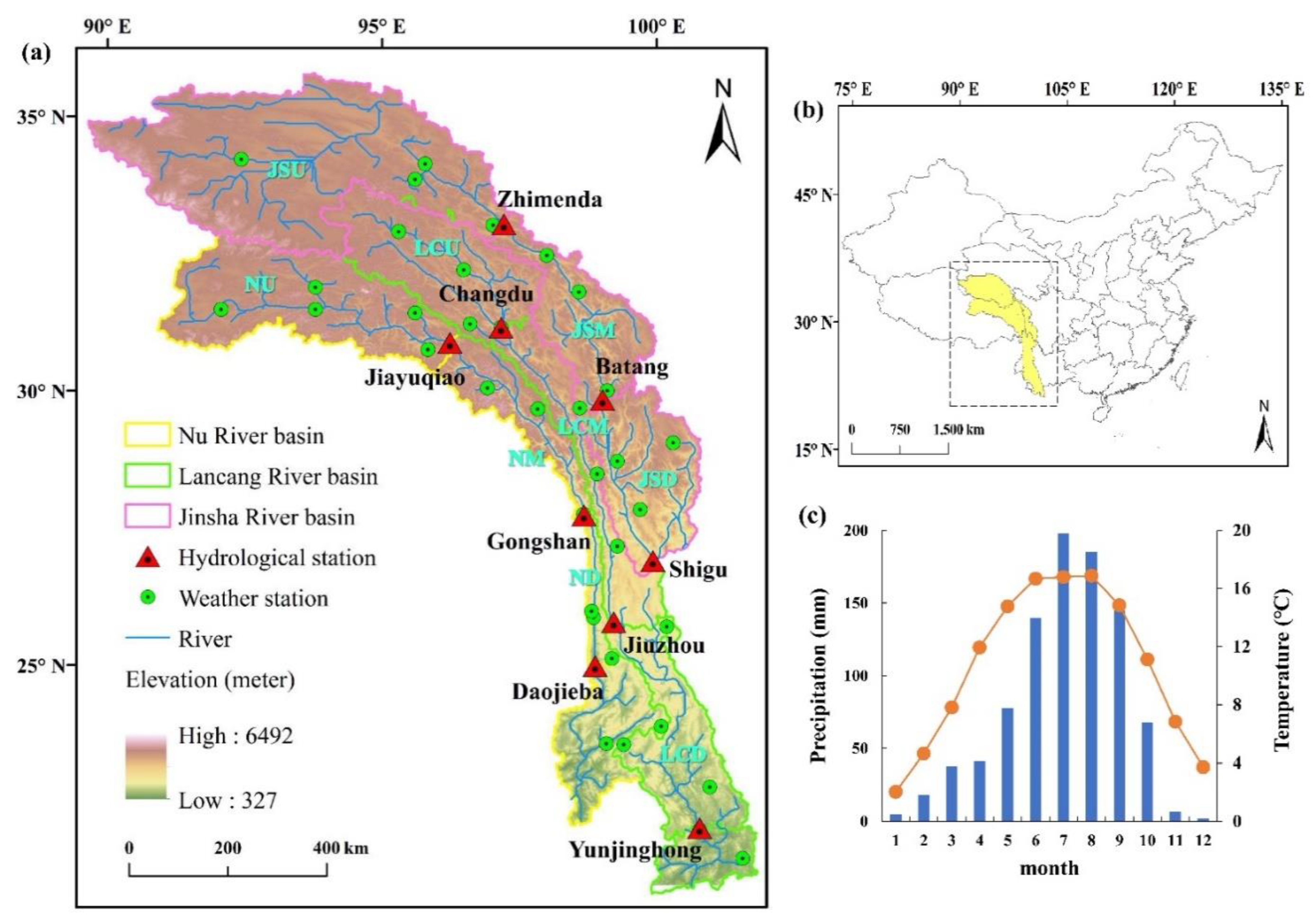
2.1. Study Area

The HDM region includes a series of parallel north–south mountain ranges in southwest China, of approximately 538,000 km². The study area includes the Nu River, Lancang River, and Jinsha River basins above Daojieba, Yunjinghong, and Shigu stations. The Nu and Lancang rivers are upstream of the Salween River and Mekong River, respectively, which are important international rivers. The terrain of this region is complex and changeable, characterized by a deep, V-shaped valley with fast surface and subsurface runoff velocities. The climate in the region varies significantly from north to south. The upstream plateau region is semiarid, with low temperatures and little precipitation. The midstream and downstream regions are subtropical and tropical climate zones in semihumid and humid regions, respectively. In general, the mean annual precipitation in the HDM region ranges from 150 mm yr⁻¹ to 1500 mm yr⁻¹, and heavy rains are concentrated during the wet season (May to October). The mean annual air temperature is between 10 °C and 30 °C from the upstream to downstream regions. Annual ET ranges from 50 mm yr⁻¹ in the north to 1500 mm yr⁻¹ in the south. The wet season ET accounts for 85% of the annual ET.

2.2. Data

2.2.1. Observed Data

Daily meteorological data for 1956 to 2018 at 35 stations in the study area were obtained from the National Meteorological Administration of China (http://data.cma.cn/ (accessed on 6 June 2021)). The data included the precipitation (mm), atmospheric pressure (Pa), mean temperature (°C) at the height of 2 meters (m), maximum temperature (°C), minimum temperature (°C), wind speed (m s⁻¹) at the height of 10 m, sunshine hours (h), and relative humidity (%).

Observed runoff data from nine hydrological stations in the mainstream basins of the HDM region were used in this study. Each hydrological station represented the mainstream control stations of the upstream, midstream, and downstream regions of the Nu, Lancang, and Jinsha rivers (Figure 1). Information on the nine hydrological sites is presented in

Table 1. Observed runoff data from nine hydrological stations.

	Hydrological Station	Longitude	Latitude	Catchment	Temporal
				Area (km2)	Coverage
Nu River Basin	Jiayuqiao	96.24	30.87	68,384	1956–2000, 2007–2018
	Gongshan	98.68	27.73	101,146	1956–2000
	Daojieba	98.88	24.98	110,224	1956–2000
Lancang River Basin	Changdu	97.17	31.15	53,800	1956–2000, 2007–2018
	Jiuzhou	99.22	25.79	88,051	1956–2000
	Yunjinghong	100.78	22.03	115,894	1956–2000
Jinsha River Basin	Zhimenda	97.22	33.03	137,704	1956–1987, 2007–2018
	Batang	99.02	29.83	187,873	1956–1987, 2007–2018
	Shigu	99.93	26.9	214,184	1956–1987, 2007–2018

. Data were obtained from the China Hydrological Yearbook.

2.2.2. RS_ET Datasets

Eight global RS_ET datasets (

Table 2. Basic information of each RS_ET dataset.

Datasets	Method	Resolution		Temporal Coverage
		Spatial	Temporal
BESS 1	PM equation	0.50°	8 days	2001–2015
	ftp://147.46.64.183 (accessed on 15 September 2020)
GLEAM 3.5a	PT equation	0.25°	1 month	1980–2020
	https://www.gleam.eu/ (accessed on 20 July 2021)
SEBS 2	Surface energy balance	0.05°	1 month	2000–2017
	https://data.tpdc.ac.cn/zh-hans/data/5a0d2e28-ebc6-4ea4-8ce4-a7f2897c8ee6/?q=%E8%92%B8%E6%95%A3 (accessed on 10 August 2020)
NTSG	Modified PM, PT equations	0.083°	1 month	1982–2013
	https://www.ntsg.umt.edu/project/global-et.php (accessed on 20 July 2021)
MOD16	PM equation	0.05°	1 month	2000–2014
	http://files.ntsg.umt.edu/data/NTSG_Products/MOD16/MOD16A2_MONTHLY.MERRA_GMAO_1kmALB/GEOTIFF_0.05degree/ (accessed on 5 August 2020)
SSEBop 3	Simplified surface energy balance	0.096°	1 month	2003–2020
	https://earlywarning.usgs.gov/fews/search (accessed on 1 November 2020)
PMLV2 4	PML model	0.05°	8 days	2002–2019
	https://data.tpdc.ac.cn/zh-hans/data/48c16a8d-d307-4973-abab-972e9449627c/?q=%E8%92%B8%E6%95%A3 (accessed on 10 August 2020)
GLASS 5	Bayesian model average	0.05°	8 days	2001–2018
	http://www.glass.umd.edu/ (accessed on 6 August 2020)

¹ Breathing Earth System Simulator; ² Surface Energy Balance System; ³ Simplified Surface Energy Balance; ⁴ Penman–Monteith–Leuning Version 2; ⁵ Global Land Surface Satellite.

), which can be downloaded freely, were used to obtain ET at the grid scale in the HDM region. The years 2000 to 2018 (datasets before 2018 were counted as the last year for which data were available) were taken as the study period.

Using the PM equation, four global RS_ET datasets (BESS, NTSG, MOD16, and PMLV2) were estimated. The BESS ET dataset [5] was estimated using the simplified process-based BESS model from the Moderate-Resolution Imaging Spectroradiometer (MODIS) atmosphere and land datasets, reanalysis, and ancillary datasets. The NTSG ET dataset [19,20] parameterized canopy conductance using the Jarvis-based stomatal conductance equation and calibrated parameters using eddy covariance measurements representing major ecological types. The MOD16 ET dataset [21,22] combined land cover, FPAR/leaf area index, albedo, and global reanalysis meteorological datasets. The PMLV2 ET dataset [6] was derived using PML model version 2. The SEBS and SSEBop ET datasets were derived using the SEB. SEBS, released by Chen et al. [23], was based on a column canopy-air turbulent diffusion method. The SSEBop ET dataset [7] was based on the inputs of the model-assimilated weather datasets and MODIS thermal images. The GLEAM ET dataset [24,25] estimated the ET for bare soil and short and tall vegetation. Multisource weighted-ensemble precipitation, surface incident shortwave and longwave radiation, and air temperature were used as forcing data to simulate the new-generation monthly ET datasets with GLEAM version 3.5a. The GLASS ET dataset was produced using a Bayesian model averaging method to improve LE estimation by merging five process-based algorithms [26,27,28].

2.3. Methods

2.3.1. Cumulative Distribution Function (CDF)-Biased WB Method

The WB_ET time series were simulated using the WB method at the basin scale. In a basin, the hydrological budget equation [29,30] can be expressed as

$${\mathrm{ET}}_i^{\mathrm{WB}}={\mathrm{P}}_i-{\mathrm{R}}_i-∆\mathrm{W}$$

(1)

where i is the sequential range; $\mathrm{P}$ and $\mathrm{R}$ are the precipitation (mm) and runoff at the basin outlet (mm), respectively; and $∆\mathrm{W}$ is the change in terrestrial water storage, including the surface subsurface, and groundwater changes (mm).

In the simulation of monthly ET, $∆\mathrm{W}$ is usually negligible [31,32]. However, the hydrological budget balance may not close when ∆W is neglected under changing climate and anthropogenic interferences such as water diversion, reservoir regulation, and agricultural irrigation. In this study, we defined (P-R) as the biased ET (${\mathrm{ET}}_{\mathrm{biased}}$) relative to the reference ET (${\mathrm{ET}}_{\mathrm{WB}}$). The ${\mathrm{ET}}_{\mathrm{biased}}$ value can be corrected based on ${\mathrm{ET}}_{\mathrm{WB}}$ measured during the same period at the monthly scale through a two-step bias correction method. Further details regarding this method were reported by Liu et al. [33].

2.3.2. Generalized CR (H2018) Method

Han et al. [34] developed a sigmoid generalized complementary function as

$$\frac{{\mathrm{ET}}^{\mathrm{H}2018}}{{\mathrm{E}}_{\mathrm{Pen}}}=\frac{1}{1+m{\left(\frac{x_{\max }-x}{x-x_{\min }}\right)}^n}$$

(2)

where ${\mathrm{E}}_{\mathrm{Pen}}$ is the evapotranspiration derived from the Penman equation (mm); $x$ is defined as the value of ${\mathrm{E}}_{\mathrm{rad}}$/${\mathrm{E}}_{\mathrm{Pen}}$, where ${\mathrm{E}}_{\mathrm{rad}}$ and ${\mathrm{E}}_{\mathrm{aero}}$ are the radiation and aerodynamic terms for the Penman equation, respectively (mm/day); $x_{\max }$ is the maximum in the x series; $x_{\min }$ is the minimum in the x series; $x_{\min }$ = 0 and $x_{\max }$ = 1 have been suggested for a daily scale; parameters $m$ and $n$ can be transferred from $\mathsf{\alpha }$ and ${\mathrm{b}}^{-1}$, where $\mathsf{\alpha }$ is a coefficient with a reasonably constant value of 1.26 for large, saturated land, and b is a parameter that denotes the linear asymmetric nature of the complementary principle [35,36,37].

$$\{\begin{array}{c}n=\frac{4\mathsf{\alpha }\left(1+{\mathrm{b}}^{-1}\right)\left(x_{0.5}-x_{\min }\right)\left(x_{\max }-x_{0.5}\right)}{\left(x_{\max }-x_{\min }\right)}\\ m={(\frac{x_{0.5}-x_{\min }}{x_{\max }-x_{0.5}})}^n\end{array}$$

(3)

where $x_{0.5}$ = ($0.5+{\mathrm{b}}^{-1}$)/ ($\mathsf{\alpha }\left(1+{\mathrm{b}}^{-1}\right)$) is the value of ${\mathrm{E}}_{\mathrm{rad}}$/${\mathrm{E}}_{\mathrm{Pen}}$ corresponding to ${\mathrm{ET}}_{\mathrm{a}}$/${\mathrm{E}}_{\mathrm{Pen}}$ = 0.5.

${\mathrm{E}}_{\mathrm{Pen}}$ and ${\mathrm{E}}_{\mathrm{aero}}$ are donated by the following equation:

$${\mathrm{E}}_{\mathrm{Pen}}={\mathrm{E}}_{\mathrm{rad}}+{\mathrm{E}}_{\mathrm{aero}}=\frac{∆}{∆+\mathsf{\gamma }}\left({\mathrm{R}}_n-\mathrm{G}\right)+\frac{\mathsf{\gamma }}{∆+\mathsf{\gamma }}\mathrm{f}\left({\mathrm{u}}_{\mathrm{z}}\right)\left({\mathrm{e}}_{\mathrm{s}}-{\mathrm{e}}_{\mathrm{a}}\right)$$

(4)

where $∆$ is the slope of the saturation vapor pressure curve at air temperature (hPa/°C), $\mathsf{\gamma }$ is the psychrometric constant (hPa/°C), ${\mathrm{R}}_n$ is the net radiation near the surface (mm/day), $\mathrm{G}$ is the soil heat flux, $\mathrm{f}\left({\mathrm{u}}_{\mathrm{z}}\right)$ is the wind function, which is calculated by Penman’s wind function [38], that is, $\mathrm{f}\left({\mathrm{u}}_2\right)$ = 0.26 (1 + 0.54${\mathrm{u}}_2$), where ${\mathrm{u}}_2$ is the wind speed at 2 m height (m/s), ${\mathrm{e}}_{\mathrm{s}}$ is the vapor pressure of the air (hPa), and ${\mathrm{e}}_{\mathrm{a}}$ is the saturation vapor pressure at air temperature (hPa). All these variables were calculated using the method recommended by the Food and Agriculture Organization (FAO) of the United Nations [39].

2.3.3. Evaluation Criteria

The performance of the monthly CR_ET and RS_ET datasets was evaluated using the WB_ET. The evaluation criteria included relative error (RE), Pearson correlation coefficient (cc [40]), root mean square error (RMSE), Nash–Sutcliffe efficiency (NSE [41]), index of agreement (IOA), Kling–Gupta efficiency (KGE [42]), and Taylor diagrams [43]. The RE value represents the deviation between the model mean and the observed mean. The value of cc indicates the degree of correlation. The RMSE, NSE, and IOA values represent the consistency between the model and the observed datasets. The KGE and Taylor diagrams are the comprehensive evaluation criteria. The Taylor diagram is a concise statistical summary of how patterns match each other in the Pearson correlation coefficient and standard deviation between the observed and modeled results.

$$\mathrm{RE}=\frac{x\left(i\right)-y\left(i\right)}{y\left(i\right)}\times 100$$

(5)

$$\mathrm{cc}=\frac{{\sum }_{i=1}^n\left[x\left(i\right)-\overline{x}\right]\left[y\left(i\right)-\overline{y}\right]}{\sqrt{{\sum }_{i=1}^n{[x\left(i\right)-\overline{x}]}^2}\sqrt{{\sum }_{i=1}^n{[y\left(i\right)-\overline{y}]}^2}}$$

(6)

$$\mathrm{RMSE}=\sqrt{\frac{1}{n}{\displaystyle \sum }_{i=1}^n{[x\left(i\right)-y\left(i\right)]}^2}$$

(7)

$$\mathrm{NSE}=1-\frac{{\sum }_{i=1}^n{[x\left(i\right)-y\left(i\right)]}^2}{{\sum }_{i=1}^n{[y\left(i\right)-\overline{y}]}^2}$$

(8)

$$\mathrm{IOA}=1-\frac{{\sum }_{i=1}^n{[x\left(i\right)-y\left(i\right)]}^2}{{\sum }_{i=1}^n(\left|x\left(i\right)-\overline{y}\right|+\left|y\left(i\right)-\overline{y}\right|{)}^2}$$

(9)

$$\mathrm{KGE}=1-\sqrt{(\mathrm{cc}-1{)}^2+(\mathsf{\alpha }-1{)}^2+(\mathsf{\beta }-1{)}^2}$$

(10)

where x(i) and y(i) are the model and observed variables at the ith time step, respectively; $\overline{x}$ and $\overline{y}$ are the model and observed mean, respectively; n is the total number of observations; α is the ratio between the variance of the model variable and observed variable, and β is the ratio between the mean of the model variable and observed variable.

2.3.4. The Method of Trends Detection

The rank-based nonparametric Mann–Kendall test [44] and trend magnitude method were applied to detect long-term monotonic trends and magnitudes. This test can handle the interference of outliers and has a high asymptotic efficiency [45]. Further details regarding this test were reported by Xu et al. [46]. The WB_ET, RS_ET, and CR_ET data were detected by the nonparametric Mann–Kendall test to investigate the spatial and temporal variations in ET at the catchment, grid, and site scale, respectively.

3. Results

3.1. Evaluation of RS_ET Datasets against Water Balance Estimates

The RE values of the RS_ET datasets against WB_ET at the three temporal scales are shown in Figure 2. Most RS_ET datasets (5/9) underestimated ET, with the mean RE values ranging from −2.34% (GLASS) to −0.07% (BESS) at the annual scale. The other four datasets overestimated ET, with the highest mean RE value of 11.76%. The mean RE values of most RS_ET datasets in the dry season were lower than the annual datasets. The datasets with the lowest RE values were SSEBop (−3.47%). However, the mean RE value of MOD16 during the dry season was higher than the annual value (5.88% vs. 0.68%). In addition, the mean RE values of RS_ET datasets in the wet season ranged from the lowest value of GLASS (−2.40%) to the highest value of NTSG (8.00%), which was similar to the annual value.

Based on the performance of the RS_ET datasets in the five small catchments, most datasets were overestimated at the annual scale. The NTSG and MOD16 values were significantly overestimated in all regions, with mean RE values ranging from 0.63% to 14.53%. Fewer RS_ET datasets were overestimated in the dry season than in the annual datasets (22 vs. 24), mainly because of the underestimation of SEBE and SSEBop. In addition, the RE values of the wet-season ET datasets were consistent with those of the annual ET datasets. Overall, except for NTSG and PMLV2, most monthly RS_ET datasets could accurately simulate ET in the HDM region. The eight RS_ET datasets outperformed the other small catchments in the LCU and JSM, with a mean RE value lower than 1.00%.

The assessment of the RS_ET datasets demonstrated by the Taylor diagrams is shown in Figure 3. In terms of the cc value, all eight RS_ET datasets agreed well with the WB_ET time series, with the cc values ranging from 0.80–0.92. The SSEBop had the best performance in five small catchments, with the cc value ranging from 0.82 to 0.95, followed by the GLASS. The NTSG performance was poorest, with the cc value not exceeding 0.85 in any catchment. The monthly RMSE value range for the eight RS_ET datasets was 15.24 mm mon⁻¹ to 29.88 mm mon⁻¹. In addition, the SSEBop performed better than other RS_ET datasets, with the RMSE value ranging from 10.07 mm mon⁻¹ to 20.31 mm mon⁻¹, followed by GLEAM. The RMSE was relatively higher in the BESS and GLASS, with 18.72 mm mon⁻¹ and 18.77 mm mon⁻¹, respectively. The NTSG performance was poorest, with an RMSE value of more than 20 mm mon⁻¹ in all small catchments; the RMSE value of the JSM was as high as 41.11 mm mon⁻¹.

The spatial variation in the performance of the RS_ ET datasets was discovered. The highest mean cc value (0.92) was in the LCU, and the lowest value of 0.81 was in the NU. The highest mean RMSE value of 29.81 mm mon⁻¹ was in the JSD, and the lowest value of 15.01 mm mon⁻¹ was in the JSU.

Overall, from the evaluation results of eight RS_ET datasets in five small catchments, the highest cc value was observed in the JSU of the SSEBop (0.95), and the lowest RMSE value was observed in the JSU of the BESS (9.33 mm mon⁻¹). Based on the Taylor diagram, SSEBop performed better than the other seven RS_ET datasets in the HDM region, followed by the GLASS dataset. The RS_ET datasets performed better in the northern semiarid region than in the humid southern region. For example, the average cc value of eight RS_ET datasets was 0.91 in JSU and 0.85 in JSD. The average RMSE value of eight RS_ET datasets in the JSU was 12.83 mm mon⁻¹, while in the JSD it was 23.85 mm mon⁻¹.

The accuracy of the RS_ET datasets in estimating monthly ET in the HDM region using the criteria of NSE, IOA, and KGE is shown in Figure 4. The results showed that SSEBop, BESS, and GLASS performed better than the other five ET datasets (Table 2). Among them, SSEBop had the best performance, with NSE, IOA, and KGE values of 0.71, 0.91, and 0.56, respectively, indicating a reasonable agreement between the SSEBop dataset and WB_ET time series at the monthly scale. The BESS followed this, with mean NSE, IOA, and KGE values of 0.67, 0.87, and 0.43, respectively. The excellent performance of GLASS was mainly reflected in high NSE and IOA values, with mean values of 0.63 and 0.86, respectively. The NTSG and MOD16 performed poorly, with mean NSE values lower than 0.50 (0.31 and 0.49), and the mean KGE for MOD16 was as low as 0.19.

Figure 5a shows that the RS_ET datasets were accurately simulated for the LCU, JSU, and JSM. In particular, in the JSU, the mean NSE value of 0.67 was higher than that in other catchments. The IOA and KGE values were similar to those of NSE (Figure 6b,c). The mean IOA values of the LCU and JSU were 0.88 and 0.87, respectively. The mean KGE values of the LCU and JSU were 0.57 and 0.62, respectively. The highest NSE value was observed for the JSU of BESS (0.83). The highest IOA value was observed in the JSU of SSEBop (0.95), and the highest KGE value was observed in the JSU of PMLV2 (0.92). Moreover, the performance of the eight RS_ET datasets in the LCU was more consistent, indicating that each dataset in this catchment could be trusted.

Overall, most RS_ET datasets can accurately simulate ET in the HDM region, except for NTSG and MOD16. SSEBop outperformed most other datasets in the five small catchments, followed by BESS and GLASS. In addition, most RS_ET datasets performed better in the LCU and JSU catchments than in the other catchments.

3.2. Evaluation of CR Series against Water Balance Estimates

In the H2018 model, the recommended $\alpha$ value of 1.26 was selected. The corresponding asymmetric parameter b with a value of 0.91 was determined [47]. The monthly CR_ET time series was obtained by weighting the area using a Voronoi diagram. The CR_ ET time series was evaluated using the WB_ET time series at monthly and seasonal scales.

As shown in Figure 6, the NSE, cc, and RMSE values of CR_ET ranged from 0.72 to 0.90, 0.84 to 0.95, and 7.20 to 11.19 mm mon⁻¹, respectively. The respective mean values were 0.90, 0.81, and 9.07 mm mon⁻¹, indicating a good consistency between the CR_ET time series and WB_ET time series. Moreover, the simulation result of CR_ET in the wet season was better than that in the dry season, with mean cc and NSE values of 0.91 and 0.87, respectively (figure not shown).

In general, the performance of CR_ET in the Lancang River Basin was better than that in the Nu River and Jinsha River basins, with mean cc, NSE, and RMSE values of 0.92, 0.83, and 9.43 mm mon⁻¹, respectively. Moreover, the highest cc and NSE values were observed in the JSD of 0.95 and 0.89, respectively. Except for the ND and JSD, the RMSE values in the other catchments were all below 10.00 mm mon⁻¹. Overall, the monthly ET time series can be accurately simulated using the H2018 model. Therefore, the CR_ET time series was applied to analyze the spatial and temporal variations in ET in the HDM region at the site scale.

3.3. Spatial and Temporal Variation of ET at Multiple Spatial Scales

The spatial patterns of annual WB_ET, CR_ET, and RS_ET in the HDM region are shown in Figure 7. As shown in Figure 7a, WB_ET increased spatially from the upstream region (182 mm yr⁻¹) to the downstream region (707 mm yr⁻¹) at the catchment scale. The CR_ET shown in Figure 7b exhibited a notably lower value (205 mm yr⁻¹) in the northern site and a higher value (1385 mm yr⁻¹) in the southern site at three temporal scales (annual, dry season, and wet season), which was similar to the findings for WB_ET. The wet season ET accounts for 70% to 90% of the annual ET.

The spatial patterns of the multiyear mean annual RS_ET datasets from 2007 to 2018 are shown in Figure 7c. There were some similarities between annual ET estimates. Most RS_ET datasets showed the lowest annual mean ET in the northwestern region of the HDM. For each dataset, the highest annual ET was observed in the downstream region. The difference between the NTSG and the seven other RS_ET datasets was concentrated in the central region. In the midstream region, the mean annual ET estimated by the NTSG ranged from 600 mm yr⁻¹ to 1000 mm yr⁻¹, while the annual ET of the other seven was lower than that of the NTSG, with values ranging from 300 mm yr⁻¹ to 600 mm yr⁻¹. In addition, SEBS underestimated annual ET in the downstream region. For example, the annual ET for MOD16 ranged from 700 mm yr⁻¹ to 1300 mm yr⁻¹, while for SEBS, it ranged from 600 mm yr⁻¹ to 1100 mm yr⁻¹ in the ND.

Trends and Mann–Kendall test results of annual ET estimated from WB_ET, CR_ET, and RS_ET in the HDM region are shown in Figure 8 and

Table 3. Mann–Kendall test results of annual ET estimated from the WB_ET, CR_ET, and RS_ET datasets.

	Catchment/Weather Station/Dataset	Sample Size	Z-Value	p-Value		Catchment/Weather Station/Dataset	Sample Size	Z-Value	p-Value
WB_ET (Catchment)	NU	57	−2.51	<0.05	CR_ET (Weather station)	56444	63	1.48	0.14
	NM	45	−0.45	0.65		56548		0.57	0.57
	ND	45	2.33	<0.05		56751		2.17	<0.05
	LCU	57	−1.36	0.17		56946		0.39	0.70
	LCM	45	0.39	0.7		56959		3.11	<0.01
	LCD	45	2.88	<0.01		56964		2.57	<0.01
	JSU	44	−0.21	0.83		56969		2.69	<0.01
	JSM	44	−1.45	0.15		56004		−1.53	0.13
	JSD	44	1.74	0.08		56016		−0.21	0.83
CR_ET (Weather station)	55299	63	−1.14	0.25		56021		−0.33	0.74
	56106		−1.42	0.16		56029		0.03	0.98
	56109		−1.24	0.22		56132		−1.24	0.22
	56116		−2.99	<0.01		56144		−1.06	0.29
	56223		−2.27	<0.05		56247		0.27	0.78
	56228		−1.68	0.09		56342		−0.33	0.74
	56331		0.58	0.59		56357		2.63	<0.05
	56533		−1.36	0.17		56441		−1.51	0.13
	56643		0.15	0.88		56543		1.84	0.07
	56741		0.33	0.73	RS_ET (Dataset)	BESS	16	−1.06	0.29
	56748		−1.17	0.24		GLEAM	19	0.17	0.86
	56945		1.6	0.11		SEBS	18	1.45	0.15
	56951		2.63	<0.01		NTSG	14	1.75	0.08
	56018		−1.78	0.08		MOD16	15	−0.05	0.96
	56125		−2.81	<0.01		SSEBop	18	0.51	0.61
	56128		−0.75	0.45		PMLV2	17	1.10	0.27
	56137		−0.63	0.53		GLASS	18	−0.09	0.92

. WB_ET (Figure 8a) exhibited an increasing trend during 1960–2018 in the Nu, Lancang, and Jinsha river basins, with magnitudes of 1.41 mm yr⁻¹, 0.60 mm yr⁻¹, and 1.37 mm yr⁻¹, respectively. A decreasing trend was observed in the upstream region. The decreasing trend was significant (significance level of 0.05, the same below) at the NU and LCU. Significant increasing trends were detected in downstream regions. Trends of ET in the dry and wet seasons (not shown) were similar to those at the annual scale. The dry-season ET decreased significantly at the LCU and JSU. In contrast, the wet-season ET decreased significantly in the NU.

Trends of ET estimated by the CR method (Figure 8b) at the site scale were generally consistent with those derived by the WB method at the catchment scale (Figure 8a). Trends of ET estimated by the CR method (Figure 8b) at the site scale were generally consistent with those derived by the WB method at the catchment scale (Figure 8a). A decreasing trend was observed at most sites in the upstream region and significantly decreased at the NU (4/5). An increasing trend of the annual CR_ET estimated by the CR model was shown in half of the sites (17/35), concentrated in the downstream region, especially in the ND and LCD. ET exhibited an increasing trend during 1960–2018 in the Nu, Lancang, and Jinsha river basins, with magnitudes of 1.53 mm yr⁻¹, 1.66 mm yr⁻¹, and 1.47 mm yr⁻¹, respectively. The dry and wet season CR_ET time series trends (not shown) were consistent with those of the annual CR_ET time series. The trend type for CR_ET showed a nonsignificant decrease (14/35), followed by a nonsignificant increase (11/35). The dry and wet season ET time series were consistent with the annual ET time series.

In general, the trends of the RS_ET datasets at the grid scale were also consistent with those at the catchment and site scales (Figure 8c). The grids with decreasing trends were concentrated in the upstream region, with the average magnitudes ranging from −4.16 mm yr⁻¹ to −1.43 mm yr⁻¹. The grids with significant increasing trends were concentrated in the midstream and downstream regions, also observed in the WB_ET and CR_ET time series. Except for BESS, MOD16, and GLASS, increasing trends of most annual RS_ET datasets were identified, with magnitudes ranging from 0.88 mm yr⁻¹ to 3.54 mm yr⁻¹. The SEBS trend was most consistent with that of the WB_ET and CR_ET time series, with the magnitude of 1.35 mm yr⁻¹, followed by the SSEBop of 1.22 mm yr⁻¹.

Moreover, the NTSG was more similar to the WB_ET time series in terms of the spatial distribution of the variation trend. Trends of ET in the dry and wet seasons (not shown) were similar to those at the annual scale. Overall, a significant decreasing trend in the northern region and an increasing trend in the southern region of the RS_ET datasets in the HDM region was observed in most regions. The variation trend at the grid scale was consistent with that at the catchment and site scales. The annual ET trend type for the NTSG was significantly increased, with a proportion of 37.6%, which for other RS_ET datasets were mainly nonsignificant, with proportions ranging from 33.3% to 63.8%. The trend types for BESS and GLASS did not significantly decrease.

Overall, annual and seasonal ET trends were generally consistent at the catchment, grid, and site scales, which were estimated by the WB method, RS_ET datasets, and CR model, respectively. They showed a significant decreasing trend in the northern semiarid region of the HDM while exhibiting an increasing trend in the humid southern region.

4. Discussion

The evaluation results of the RS_ET datasets in this study were compared with those of existing studies. Abdelrazek et al. [48] evaluated the GLEAM, SEBS, NTSG, MOD16, and SSEBop on a global scale, with the RMSE values of 31.23 mm mon⁻¹, 34.03 mm mon⁻¹, 29.22 mm mon⁻¹, 32.72 mm mon⁻¹, and 33.85 mm mon⁻¹, respectively. In this study, these RS_ET datasets had higher accuracy in the HDM region than the global datasets with lower RMSE values. Hyun et al. [49] verified that the MOD16 dataset in Asia and the RMSE value in the Haibei region of southern China were close to that of the HDM region (7.66 mm 8 day⁻¹ vs. 20.04 mm mon⁻¹). Bai et al. [11] found that the GLEAM performed better than other RS_ET datasets in the Xishuangbanna district with cc and KGE values of 0.81 and 0.47, respectively. In this study, GLEAM’s cc and KGE values were 0.88 and 0.47, respectively, downstream of the Lancang River Basin. In this region, the Xishuangbanna district was located. Yin et al. [50] demonstrated that the SSEBop dataset had a better performance in the Yellow River Basin, with RMSE and RE values of 63.25 mm yr⁻¹ and 3.01%, respectively. The RMSE and RE values of the RS_ET datasets were higher in the HDM region than in the Yellow River Basin.

A worldwide evaluation showed that RS_ET datasets had higher accuracy in dry basins than in energy-limited wet basins [51]. The better performance of ET datasets in arid regions than in humid areas was also found at a regional scale, such as Iran [52]. This study demonstrated better performance in simulating monthly time series in semiarid regions than in humid regions. For example, the mean NSE value upstream of the Jinsha River Basin was 0.80, while the downstream value was 0.68. In addition, Miralles et al. [4] reported that GLEAM and MOD16 showed divergence under water-stress and drought conditions. There may be potential water stress in large areas of the HDM region affected by the hot–dry valley climate. The present study provides an explanation for the low ranking of GLEAM and MOD16.

Some studies have suggested that RS_ET datasets with higher spatial resolution do not necessarily perform better than those with lower resolution [8,53,54]. For example, in this study, the coarser-resolution dataset of GLEAM outperformed the higher-resolution datasets of SEBS and PMLV2 in the HDM region. Thus, higher-resolution datasets do not always outperform lower-resolution datasets. The spatial resolution of the ET estimates used may not be a critical element in determining which dataset was used for a particular requirement. Currently, remote-sensing products with higher spatial resolutions, such as Landsat [55] and ECOSTRESS [56], have been studied. The development of higher-resolution RS_ET datasets using these higher-resolution images would benefit local applications of ET products.

The comprehensive ranking for each ET time series was based on the average ranking of the different evaluation criteria, including, but not limited to, the cc and NSE values. The ranking of the top four or the lowest-ranked series was not affected by sorting by different indicators. For example, the following RS_ET datasets had the highest cc values in the following order: SSEBop, GLASS, GLEAM, and BESS. The RS_ET datasets had the highest NSE values in the following order: SSEBop, BESS, GLASS, and GLEAM datasets, and had the highest IOA values in the following order: SSEBop, GLEAM, PMLV2, and BESS. It is worth noting that the sorting results were different when only the KGE value was considered. PMLV2 ranked first, followed by SSEBop, GLEAM, and SEBS. The lowest-ranked dataset was the NTSG for all criteria.

When climate conditions were similar in some catchments, the evaluation results of the RS_ET datasets were consistent. For example, the upstream regions of the three rivers were in similar climatic zones and topographic conditions, and the performance of the RS_ET datasets was similar for each catchment. The following RS_ET datasets had the highest NSE values in the specified order in the NU: GLASS, SSEBop, and BESS. In the LCU, the specified orders were SSEBop, GLASS, and BESS. In the JSU, the specified order was BESS, SSEBop, and GLASS. However, for the upstream, midstream, and downstream basin regions, the assessment results of the RS_ET datasets varied slightly, owing to water stress, topography, climate, and other factors. For example, in JSU, the highest NSE values of the RS_ET datasets in the specified order were BESS, SSEBop, and GLEAM. However, in the JSD, the specified orders were MOD16, SSEBop, and BESS.

Precipitation and evapotranspiration during the wet season accounted for more than 80% of the annual values. The wet season is the season for plant growth and is of great significance in agriculture and forestry. Most RS_ET datasets had relatively small errors during the wet season in the study area. However, they showed relatively greater errors during the dry season. Therefore, the accuracy of the RS_ET datasets might require further improvements in the dry season when the soil water is limited.

The uncertainties of the WB_ET simulation were mainly due to uncertainties in the input data and during the simulation processes. The cumulative distribution function (CDF)-biased WB method was applied to reduce uncertainty in this study. The uncertainties of the RS_ET datasets are sourced from several parts. RS_ET datasets are generally estimated from surface variables, including surface temperature and vegetation index. The surface variables retrieved from remote-sensing images may contain uncertainties. The parameterization schemes in remote-sensing models also have some uncertainties. In addition, the remote-sensing technique can only detect the instantaneous ET rate at the time of satellite overpasses. Temporal upscaling of instantaneous ET over some time (e.g., daily) is necessary for remote-sensing ET maps [9]. This would also induce uncertainties in the RS_ET datasets.

Global RS_ET datasets can provide the spatial distribution of ET. RS_ET datasets are currently the only means of monitoring ET’s temporal and spatial characteristics on a global scale. Global RS_ET datasets have important application value in agricultural irrigation, integrated water resource management, and ecological environment monitoring. However, the accuracy of the global RS_ET dataset needs to be assessed before it can be applied to specified regions. The results showed that most global RS_ET datasets overestimated the actual evapotranspiration of the HDM region as a whole, with an average relative error of only 1.57%, which can be used for spatiotemporal regional ET monitoring.

5. Conclusions

This study focused on the evaluation of RS-based global datasets at the catchment scale in mountainous regions. The eight global RS-based ET datasets generated using satellite imagery and ground-based observations, which are freely accessible to the public, were comprehensively assessed by monthly ET time series simulated by the WB method at the catchment scale in the HDM region. The CR model, which derived ET from meteorological data, was also evaluated for WB-based ET. In addition, the WB_ET, CR_ET, and RS_ET datasets were used to investigate spatial and temporal variations at the catchment, grid, and site scale in the HDM region, respectively.

(1)

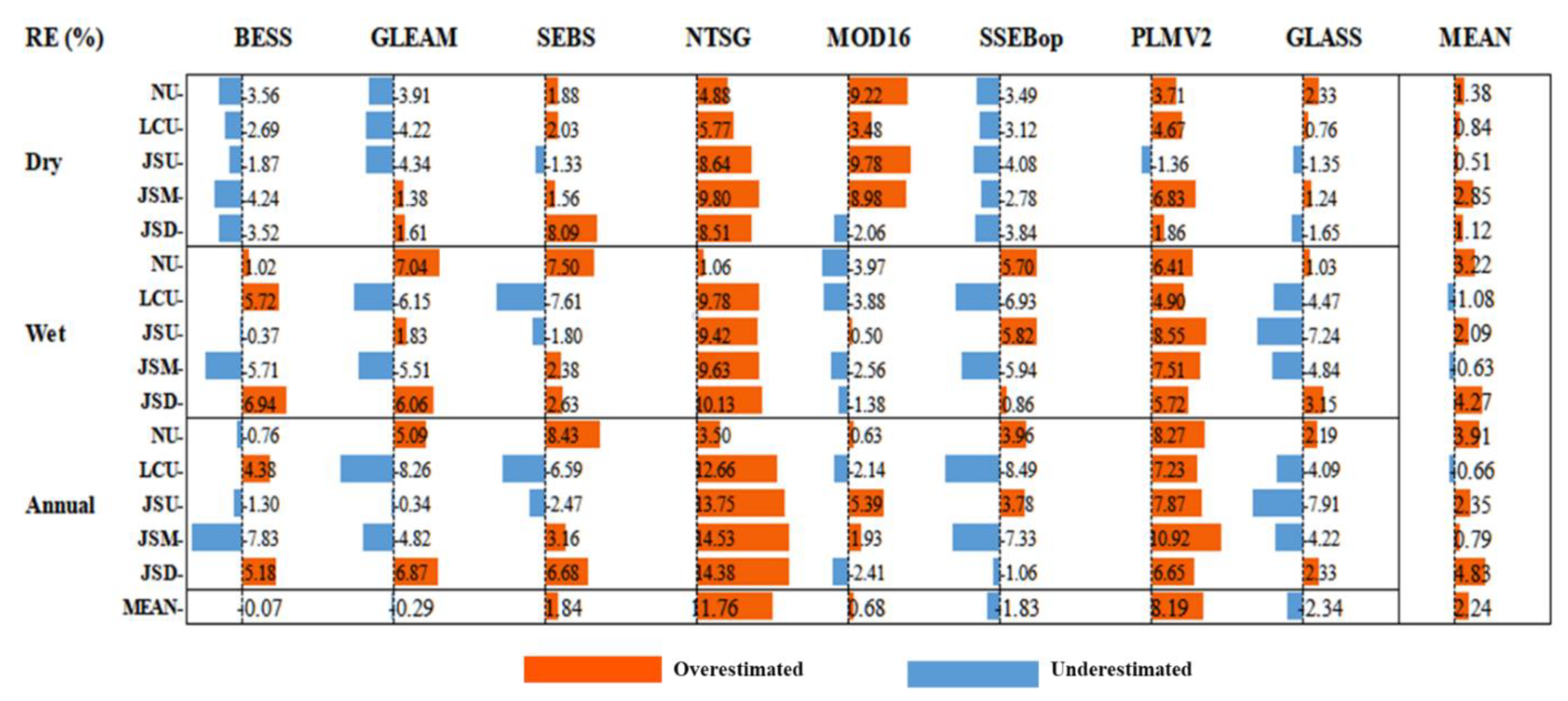
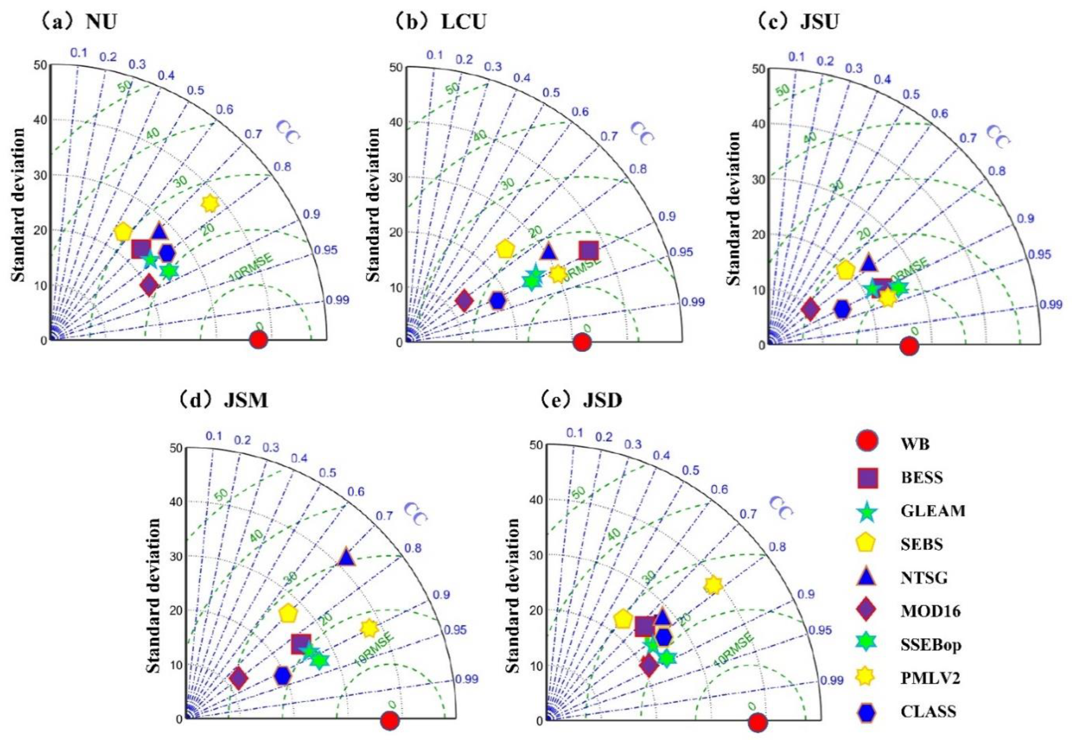
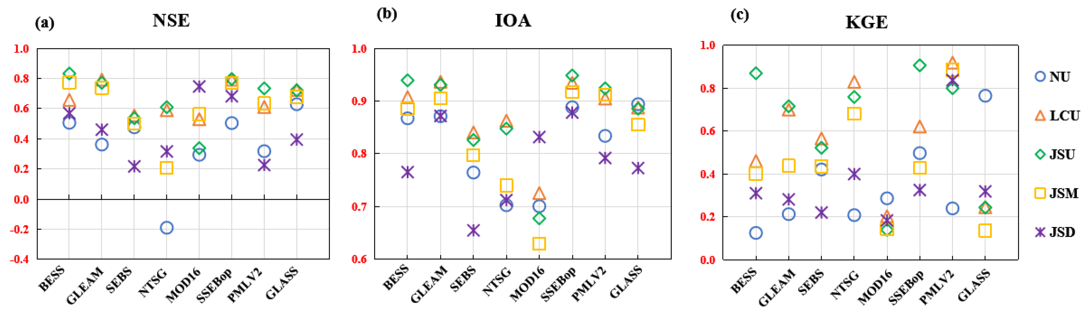
The RS_ET datasets accurately simulated ET at the monthly scale in the HDM region, with mean cc and NSE values of 0.89 and 0.68, respectively. The SSEBop outperformed the others, with NSE and KGE values of 0.80 and 0.90, respectively. This was followed by GLASS and BESS. The NTSG and MOD16 performed worse, with mean RE values of more than 10.0% and mean NSE values below 0.50. In addition, the RS_ET datasets showed high accuracy in estimating the mean values in both the semiarid and humid regions. RT_ES showed relatively better performance in simulating monthly time series in semiarid regions than in humid regions, with the mean NSE value of the former being 0.78.

(2)

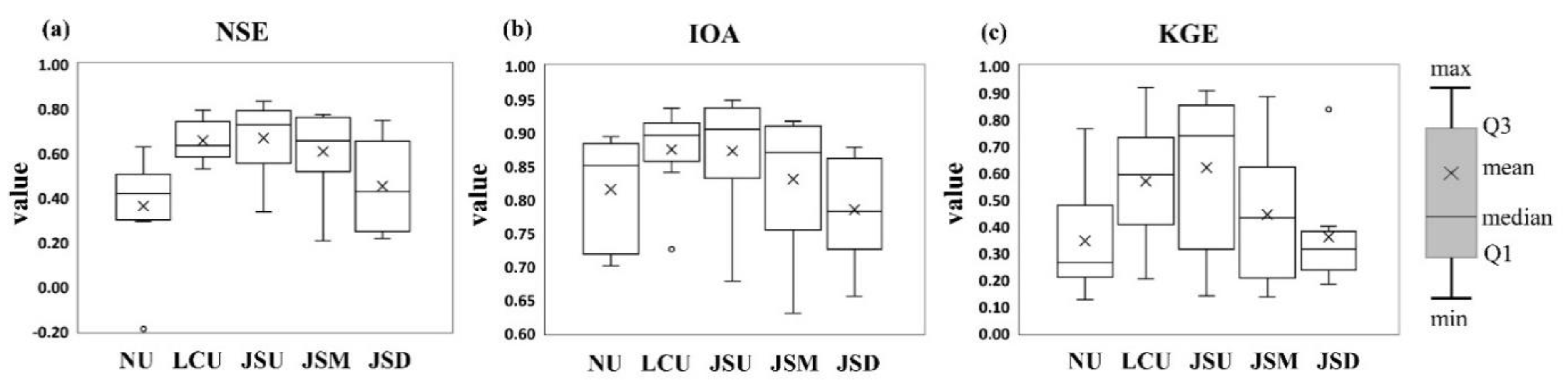
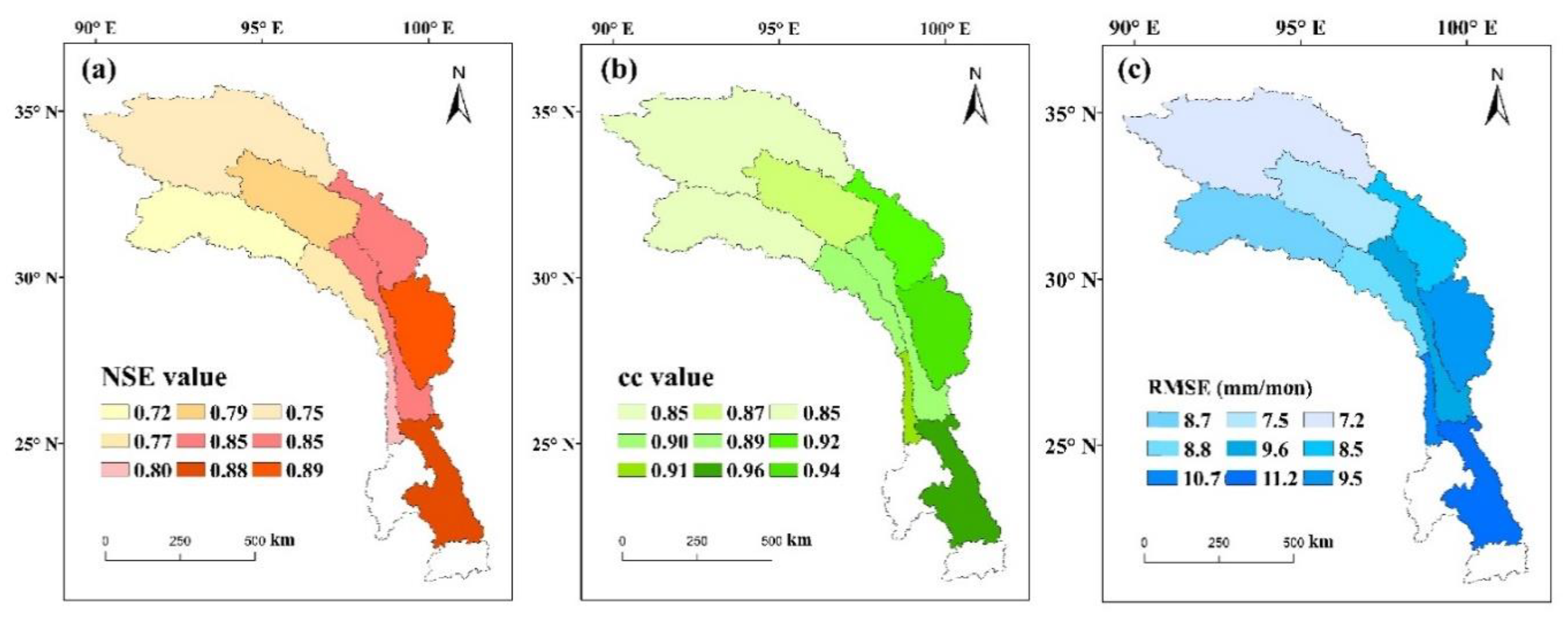
The CR model was also able to accurately simulate ET at the monthly scale in the HDM region, with mean cc, NSE, and RMSE values of 0.90, 0.81, and 9.07 mm mon⁻¹, respectively. The simulation results of CR_ET in the wet season were better than those in the dry season, with cc and NSE values of 0.91 and 0.76, respectively. Moreover, the comprehensive performance of CR_ET in the Lancang River Basin was better, with mean cc and NSE of 0.92 and 0.83, respectively.

(3)

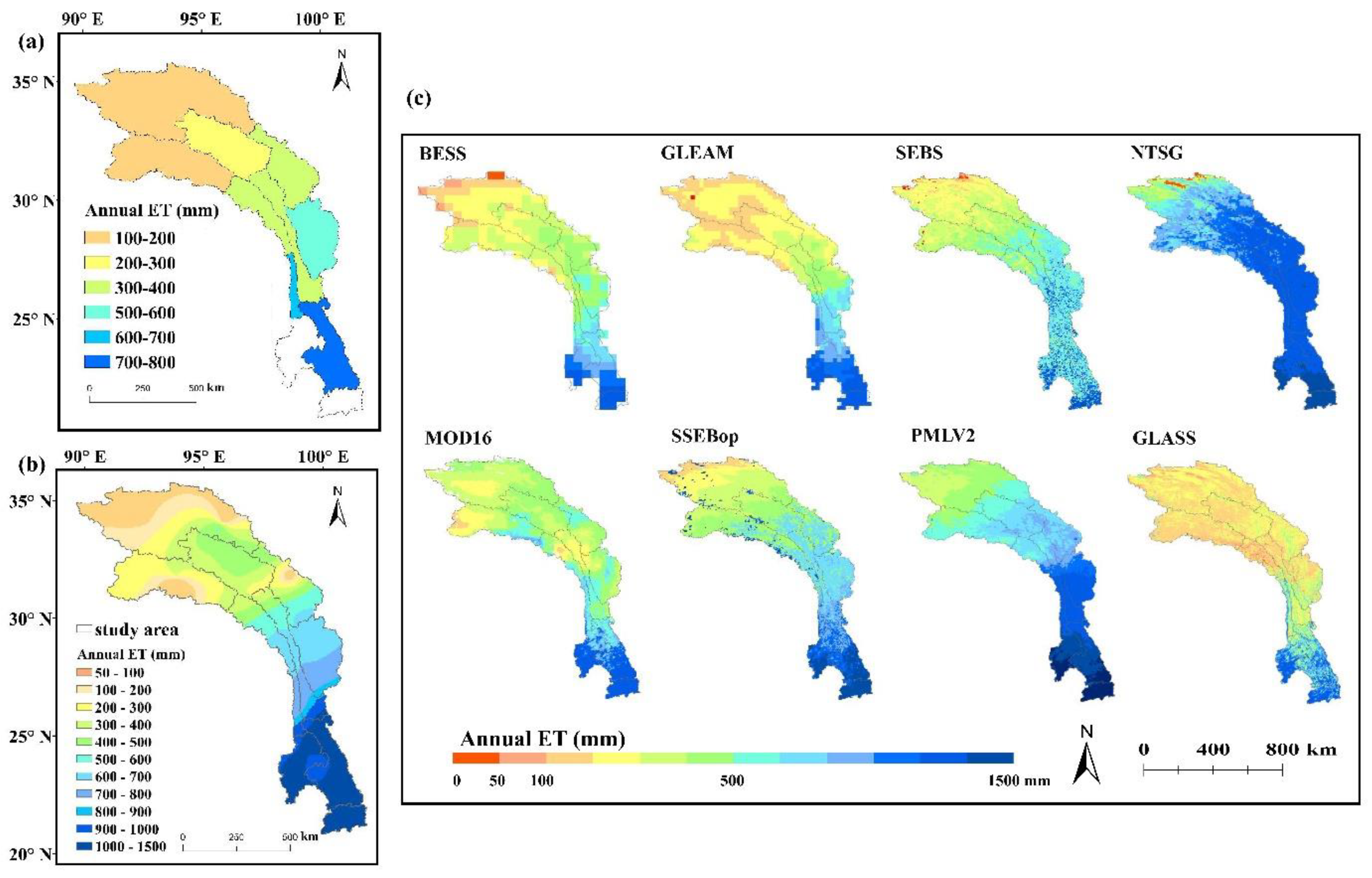
The spatial and temporal variations of the ET time series, including WB_ET, CR_ET, and RS_ET, were generally consistent in the HDM region. All ET time series showed a significant decreasing trend in the northern semiarid region of the HDM, with the lowest mean annual ET. Meanwhile, they exhibited an increasing trend in the humid southern region, with the highest mean annual ET.

References

1. Oki, T.; Kanae, S. Global hydrological cycles and world water resources. Science 2006, 313, 1068–1072. [Google Scholar] [CrossRef] [Green Version]
2. Trenberth, K.E.; Fasullo, J.T.; Kiehl, J. Earth’s global energy budget. Bull. Am. Meteorol. Soc. 2009, 90, 311–323. [Google Scholar] [CrossRef]
3. Katul, G.G.; Oren, R.; Manzoni, S.; Higgins, C.; Parlange, M.B. Evapotranspiration: A process driving mass transport and energy exchange in the soil-plant-atmosphere-climate system. Rev. Geophys. 2012, 50, RG3002. [Google Scholar] [CrossRef] [Green Version]
4. Miralles, D.G.; Jiménez, C.; Jung, M.; Michel, D.; Ershadi, A.; McCabe, M.F.; Hirschi, M.; Martens, B.; Dolman, A.J.; Fisher, J.B. The WACMOS-ET project-Part 2: Evaluation of global terrestrial evaporation data sets. Hydrol. Earth Syst. Sci. 2020, 20, 823–842. [Google Scholar] [CrossRef] [Green Version]
5. Ryu, Y.; Baldocchi, D.D.; Kobayashi, H.; Van Ingen, C.; Li, J.; Black, T.A.; Beringer, J.; van Gorsel, E.; Knohl, A.; Law, B.E. Integration of MODIS land and atmosphere datasets with a coupled-process model to estimate gross primary data setsivity and evapotranspiration from 1 km to global scales. Global Biogeochem. Cycles. 2011, 25, GB4017. [Google Scholar] [CrossRef] [Green Version]
6. Zhang, Y.Q. PML_V2 global evapotranspiration and gross primary data setsion (2002.07–2019.08). Natl. Tibet. Plateau Data Center 2020, 56, e2020WR028205. [Google Scholar] [CrossRef]
7. Senay, G.B.; Bohms, S.; Singh, R.K.; Gowda, P.H.; Velpuri, N.M.; Alemu, H.; Verdin, J.P. Operational Evapotranspiration Mapping Using Remote Sensing and Weather Datasets: A New Parameterization for the SSEB Approach. J. Am. Water Resour. Assoc. 2013, 49, 577–591. [Google Scholar] [CrossRef] [Green Version]
8. Panahi, M.D.; Tabas, S.S.; Kalantari, Z.; Ferreira, C.S.S.; Zahabiyoun, B. Spatio-temporal assessment of global gridded evapotranspiration datasets across Iran. Remote Sens. 2021, 13, 1816. [Google Scholar] [CrossRef]
9. Liu, Z.F. The accuracy of temporal upscaling of instantaneous evapotranspiration to daily values with seven upscaling methods. Hydrol. Earth Syst. Sci. 2021, 25, 4417–4433. [Google Scholar] [CrossRef]
10. Imeshi, W.; Wim, B.; Marloes, M.; Jia, L.; van Ann, G. Can we trust remote sensing evapotranspiration products over Africa? Hydrol. Earth Syst. Sci. 2020, 24, 1565–1586. [Google Scholar] [CrossRef] [Green Version]
11. Koppa, A.; Alam, S.; Miralles, D.G.; Gebremichael, M. Budyko-based long-term water and energy balance closure in global watersheds from Earth observations. Water Resour. Res. 2021, 57, e2020WR028658. [Google Scholar] [CrossRef] [PubMed]
12. Luo, Z.; Shao, Q.; Wan, W.; Li, H.; Chen, X.; Zhu, S.; Ding, X. A new method for assessing satellite-based hydrological data products using water budget closure. J. Hydrol. 2021, 594, 125927. [Google Scholar] [CrossRef]
13. Schoups, G.; Nasseri, M. GRACEfully closing the water balance: A data-driven probabilistic approach applied to river basins in Iran. Water Resour. Res. 2021, 57, e2020WR029071. [Google Scholar] [CrossRef]
14. Bai, P.; Liu, X.M. Intercomparison and evaluation of three global high-resolution evapotranspiration data sets across China. J. Hydrol. 2018, 566, 743–755. [Google Scholar] [CrossRef]
15. Baik, J.; Umar, W.L.; Minha, C. Assessment of satellite- and reanalysis-based evapotranspiration productswith two blending approaches over the complex landscapes and climates of Australia. Agric. For. Meteorol. 2018, 263, 388–398. [Google Scholar] [CrossRef]
16. Sorensson, A.A.; Ruscica, R.C. Intercomparison and uncertainty assessment of nine evapotranspiration estimates over South America. Water Resour. Res. 2018, 54, 2891–2908. [Google Scholar] [CrossRef] [Green Version]
17. Xu, T.R.; Guo, Z.X.; Xia, Y.L.; Vagner, G.F.; Liu, S.M.; Wang, K.C.; Yao, Y.J.; Zhang, X.J.; Zhao, C.S. Evaluation of twelve evapotranspiration data sets from machine learning. J. Hydrol. 2019, 578, 124105. [Google Scholar] [CrossRef]
18. Wu, J.; Venkataraman, L.; Wang, D.S.; Lin, P.R.; Pan, M.; Cai, X.T.; Wood, E.F.; Zeng, Z.Z. The Reliability of Global RS Evapotranspiration Data sets over Amazon. Remote Sens. 2020, 12, 2211. [Google Scholar] [CrossRef]
19. Zhang, K.; Kimball, J.S.; Nemani, R.R.; Running, S.W. A continuous satellite-derived global record of land surface evapotranspiration from 1983 to 2006. Water Resour. Res. 2010, 46, W09522. [Google Scholar] [CrossRef] [Green Version]
20. Zhang, K.; Kimball, J.S.; Nemani, R.R.; Running, S.W.; Hong, Y.; Gourley, J.J.; Yu, Z.B. Vegetation greening and climate change promote multidecadal rises of global land evapotranspiration. Sci. Rep. 2015, 5, 15956. [Google Scholar] [CrossRef]
21. Mu, Q.; Heinsch, F.A.; Zhao, M.; Running, S.W. Development of a global evapotranspiration algorithm based on MODIS and global meteorology data. Remote Sens. Environ. 2007, 111, 519–536. [Google Scholar] [CrossRef]
22. Mu, Q.; Heinsch, F.A.; Zhao, M.; Running, S.W. Improvements to a MODIS global terrestrial evapotranspiration algorithm. Remote Sens. Environ. 2011, 115, 1781–1800. [Google Scholar] [CrossRef]
23. Chen, X.L. Surface energy balance based global land evapotranspiration (EB-ET 2000–2017). Natl. Tibet. Plateau Data Center 2018. [Google Scholar] [CrossRef] [Green Version]
24. Martens, B.; Miralles, D.G.; Lievens, H.; Van Der Schalie, R.; De Jeu, R.A.M.; Fernández-Prieto, D.; Beck, H.E.; Dorigo, W.A.; Verhoest, N.E.C. GLEAM v3: Satellite-based land evaporation and root-zone soil moisture. Geosci. Model Dev. 2017, 10, 1903–1925. [Google Scholar] [CrossRef] [Green Version]
25. Miralles, D.G.; Holmes, T.R.H.; De Jeu, R.A.M.; Gash, J.H.; Meesters, A.G.C.A.; Dolman, A.J. Hydrology and Earth System Sciences Global land-surface evaporation estimated from satellite-based observations. Hydrol. Earth Syst. Sci. 2011, 15, 453–469. [Google Scholar] [CrossRef] [Green Version]
26. Yao, Y.J.; Liang, S.L.; Cheng, J.; Liu, S.; Fisher, J.B.; Zhang, X.T.; Jia, K. MODIS-driven estimation of terrestrial latent heat flux in China based on a modified Priestley-Taylor algorithm. Agric. For. Meteorol. 2013, 171, 187–202. [Google Scholar] [CrossRef]
27. Yao, Y.J.; Liang, S.L.; Li, X.L.; Hong, Y.; Fisher, J.B.; Zhang, N.N.; Chen, J.Q.; Cheng, J.; Zhao, S.H.; Zhang, X.T. Bayesian multimodel estimation of global terrestrial latent heat flux from eddy covariance, meteorological, and satellite observations. J. Geophys. Res. Atmos. 2014, 119, 4521–4545. [Google Scholar] [CrossRef]
28. Liang, S.; Cheng, C.; Jia, K.; Jiang, B.; Liu, Q.; Xiao, Z.; Yao, Y.; Yuan, W.; Zhang, X.; Zhao, X.; et al. The Global LAnd Surface Satellite (GLASS) products suite. Bull. Am. Meteorol. Soc. 2021, 102, E323–E337. [Google Scholar] [CrossRef]
29. Liu, Z.F.; Yao, Z.J.; Wang, R. Simulation and evaluation of actual evapotranspiration based on inverse hydrological modeling at a basin scale. Catena 2019, 180, 160–168. [Google Scholar] [CrossRef]
30. Wan, Z.M.; Zhang, K.; Xue, X.W.; Hong, Z.; Hong, Y.; Gourley, J.J. Water balance based actual evapotranspiration reconstruction from ground and satellite observations over the Conterminous United States. Water Resour. Res. 2015, 51, 6485–6499. [Google Scholar] [CrossRef]
31. Hobbins, M.; Ramirez, J.; Brown, T.; Claessens, L. The complementary relationship in estimation of regional evapotranspiration: The complementary relationship areal evapotranspiration and advection-aridity models. Water Resour. Res. 2001, 37, 1367–1387. [Google Scholar] [CrossRef] [Green Version]
32. Zhang, Y.Q.; Leuning, R.; Chiew, F.H.S.; Wang, E.L.; Zhang, L.; Liu, C.M.; Sun, F.B.; Peel, M.C.; Shen, Y.J.; Jung, M. Decadal trends in evaporation from global energy and water balances. J. Hydrometeorol. 2012, 13, 379–391. [Google Scholar] [CrossRef]
33. Liu, X.M.; Liu, C.M.; Brutsaert, W. Regional evaporation estimates in the eastern monsoon region of China: Assessment of a nonlinear formulation of the complementary principle. Water. Resour. Res. 2016, 52, 9511–9521. [Google Scholar] [CrossRef]
34. Han, S.J.; Tian, F.Q. Derivation of a sigmoid generalized complementary function for evaporation with physical constraints. Water Resour. Res. 2018, 54, 5050–5068. [Google Scholar] [CrossRef]
35. Kahler, D.M.; Brutsaert, W. Complementary relationship between daily evaporation in the environment and pan evaporation. Water Resour. Res. 2006, 42, W05413. [Google Scholar] [CrossRef]
36. Szilagyi, J. On the inherent asymmetric nature of the complementary relationship of evaporation. Geophys. Res. Lett. 2007, 34, L02405. [Google Scholar] [CrossRef] [Green Version]
37. Szilagyi, J. Complementary-relationship-based 30 year normals (1981–2010) of monthly latent heat fluxes across the contiguous United States. Water Resour. Res. 2015, 51, 9367–9377. [Google Scholar] [CrossRef] [Green Version]
38. Penman, H. Natural evaporation from open water, bare soil and grass. Proc. R. Soc. Lond. A. Math. Phys. Sci. 1948, 193, 120–145. [Google Scholar]
39. Allen, R.G. Using the FAO-56 dual crop coefficient method over an irrigated region as part of an evapotranspiration intercomparison study. J. Hydrol. 2000, 229, 27–41. [Google Scholar] [CrossRef]
40. Pearson, K. Mathematical Contributions to the Theory of Evolution-On a Form of Spurious Correlation Which May Arise When Indices Are Used in the Measurement of Organs. Lond. R. Soc. Lond. Proc. 1896, 60, 489–498. [Google Scholar]
41. Nash, J.E.; Sutcliffe, J.V. River flow forecasting through conceptual models part I-A discussion of principles. J. Hydrol. 1970, 10, 282–290. [Google Scholar] [CrossRef]
42. Gupta, H.V.; Kling, H.; Yilmaz, K.K.; Martinez, G.F. Decomposition of the mean squared error and NSE performance criteria: Implications for improving hydrological modelling. J. Hydrol. 2009, 377, 80–91. [Google Scholar] [CrossRef] [Green Version]
43. Taylor, K.E. Summarizing multiple aspects of model performance in a single diagram. J. Geophys. Res. Atmos. 2001, 106, 7183–7192. [Google Scholar] [CrossRef]
44. Hirsch, R.M.; Slack, J.R.; Smith, R.A. Techniques of trend analysis for monthly water quality data. Water Resour. Res. 1982, 18, 107–121. [Google Scholar] [CrossRef] [Green Version]
45. Fu, G.B.; Charles, S.P.; Liu, C.M.; Yu, J.J. Decadal climatic variability, trends and future scenarios for the North China Plain. J. Clim. 2009, 22, 2111–2123. [Google Scholar] [CrossRef]
46. Xu, Z.X.; Liu, Z.F.; Fu, G.B.; Chen, Y.N. Hydro-climate trends of the Tarim River basin for the last 50 years. J. Arid. Environ. 2010, 74, 256–267. [Google Scholar] [CrossRef]
47. Wang, L.M.; Tian, F.Q.; Han, S.J.; Wei, Z.W. Determinants of the asymmetric parameter in the generalized complementary principle of evaporation. Water Resour. Res. 2020, 56, e2019WR026570. [Google Scholar] [CrossRef]
48. Elnashar, A.; Wang, L.J.; Wu, B.F.; Zhu, W.W.; Zeng, H.W. Synthesis of global actual evapotranspiration from 1982 to 2019. Earth Syst. Sci. Data. 2021, 13, 447–480. [Google Scholar] [CrossRef]
49. Kim, H.W.; Hwang, K.; Mu, Q.; Seung, O.; Lee, S.O. Validation of MODIS 16 Global Terrestrial Evapotranspiration Products in Various Climates and Land Cover Types in Asia. J. Civi. Eng. 2012, 16, 229–238. [Google Scholar] [CrossRef]
50. Yin, L.C.; Wang, X.F.; Feng, X.M.; Fu, B.J.; Chen, Y.Z. A Comparison of SSEBoPModel-Based Evapotranspiration with Eight Evapotranspiration Data sets in the Yellow River Basin, China. Remote Sens. 2020, 12, 2528. [Google Scholar] [CrossRef]
51. Liu, W.B.; Wang, L.; Zhou, J.; Li, Y.Z.; Sun, F.B.; Fu, G.B.; Li, X.P.; Sang, Y.F. A worldwide evaluation of basin-scale evapotranspiration estimates against the water balance method. J. Hydrol. 2016, 538, 82–95. [Google Scholar] [CrossRef] [Green Version]
52. Gan, R.; Zhang, Y.Q.; Shi, H.; Yang, Y.T.; Eamus, D.; Cheng, L.; Chiew, F.H.S. Use of satellite leaf area index estimating evapotranspiration and gross assimilation for Australian ecosystems. Ecohydrology 2018, 11, e1974. [Google Scholar] [CrossRef]
53. Khan, M.S.; Baik, J.; Choi, M. Inter-comparison of evapotranspiration datasets over heterogeneous landscapes across Australia. Adv. Space. Res. 2020, 66, 533–545. [Google Scholar] [CrossRef]
54. Baker, J.C.A.; Garcia-Carreras, L.; Gloor, M.; Marsham, J.H.; Buermann, W.; da Rocha, H.R.; Nobre, A.D.; de Araujo, A.C.; Spracklen, D.V. Evapotranspiration in the Amazon: Spatial patterns, seasonality, and recent trends in observations, reanalysis, and climate models. Hydrol. Earth Syst. Sci. 2021, 25, 2279–2300. [Google Scholar] [CrossRef]
55. Senay, G.B.; Friedrichs, M.; Singh, R.K.; Velpuri, N.M. Evaluating Landsat 8 evapotranspiration for water use mapping in the Colorado River Basin. Remote Sens. Environ. 2016, 185, 171–185. [Google Scholar] [CrossRef] [Green Version]
56. Fisher, J.B.; Lee, B.; Purdy, A.J.; Halverson, G.H.; Dohlen, M.B.; Cawse-Nicholson, K.; Wang, A.; Anderson, R.G. ECOSTRESS: NASA’s Next Generation Mission to Measure Evapotranspiration from the International Space Station. Water Resour. Res. 2020, 56, 4. [Google Scholar] [CrossRef]
Figure 1. (a) Location of each catchment, hydrological station, and weather station (DEM data: https://ciat.cgiar.org/ (accessed on 1 November 2020)), (b) map of China, and (c) precipitation and temperature time series. The catchment was defined by hydrological stations in the main stream. NU, NM, and ND represent the upstream, midstream, and downstream regions of the Nu River Basin, respectively. LCU, LCM, and LCD represent the upstream, midstream, and downstream regions of the Lancang River Basin, respectively. JSU, JSM, and JSD represent the upstream, midstream, and downstream regions of Jinsha River Basin, respectively.
Remotesensing 13 05096 g001
Figure 2. Relative error of RS_ET datasets at annual and seasonal scale (the dry season is from November to April; the wet season is from May to October).
Remotesensing 13 05096 g002
Figure 3. Taylor diagram of eight RS_ET datasets for (a) NU, (b) LCU, (c) JSU, (d) JSM, and (e) JSD, for which water-balance-derived ET was evaluated at a monthly scale (the radiating lines in the Taylor diagram represent the correlation coefficient, the horizontal and vertical axes represent the standard deviation, and the dotted lines represent the root mean square error).
Remotesensing 13 05096 g003
Figure 4. Accuracy of eight RS_ET datasets in estimating monthly datasets at each catchment by the criteria of (a) NSE, (b) IOA, and (c) KGE.
Remotesensing 13 05096 g004
Figure 5. Performance of RS_ET datasets by the index of (a) NSE, (b) IOA, and (c) KGE in each catchment.
Remotesensing 13 05096 g005
Figure 6. Evaluation of the H2018 model by the index of (a) NSE, (b) cc, and (c) RMSE.
Remotesensing 13 05096 g006
Figure 7. Annual ET estimated by (a) WB_ET, (b) CR_ET, and (c) RS_ET datasets in the HDM region.
Remotesensing 13 05096 g007
Figure 8. Trends of annual ET estimated from the (a) WB_ET, (b) CR_ET, and (c) RS_ET datasets in the HDM region (basins in red, blue, pink, and light blue represent significant increasing, significant decreasing, increasing, and decreasing trends, respectively).
Remotesensing 13 05096 g008