Predicting Plant Growth from Time-Series Data Using Deep Learning


Abstract
:
1. Introduction
- Novel Dataset and Innovative Preprocessing: Most of the studies in plant phenotyping based remote sensing focuses only on a few available plant datasets. We acquired the Arabidopsis dataset and used the latest machine learning software to annotate it. The overall annotation was automatic, and it produces image and XML based annotations that can be interoperable between different software tools. In this way, the recorded plant data (especially roots) can be used for future analysis and experiments.
- Innovative Deep Learning Models: The field of remote sensing constantly innovates through the development and application of innovative machine learning models. GANs are one of the least experimented with machine learning methods for plant phenotyping. The proposed research’s key objective is to showcase the strength and diversity of GANs and utilize it to enhance phenotyping productivity. The higher resolution output produced by the progressively growing GAN architecture adopted and improved is also one of the proposed method’s key contributions.
- Comprehensive Results: The proposed system is designed to incorporate and utilize both spatial and temporal plant data to forecast growth. It offers an accurate and efficient predictive segmentation of plant data (root/leaf). Accurate prediction of future plant growth could substantially reduce the time required to conduct growth experiments, with plants requiring less growing time and new experimental cycles beginning sooner.
- Generalization and Reproducibility: The proposed system (designed in PyTorch and Python) is freely available on GitHub. It is a robust machine learning-based system that may be reapplied to any dataset with only minor modifications. We demonstrate this through the application of this system on two very different datasets of plant shoots and roots respectively.
2. Background
3. Method
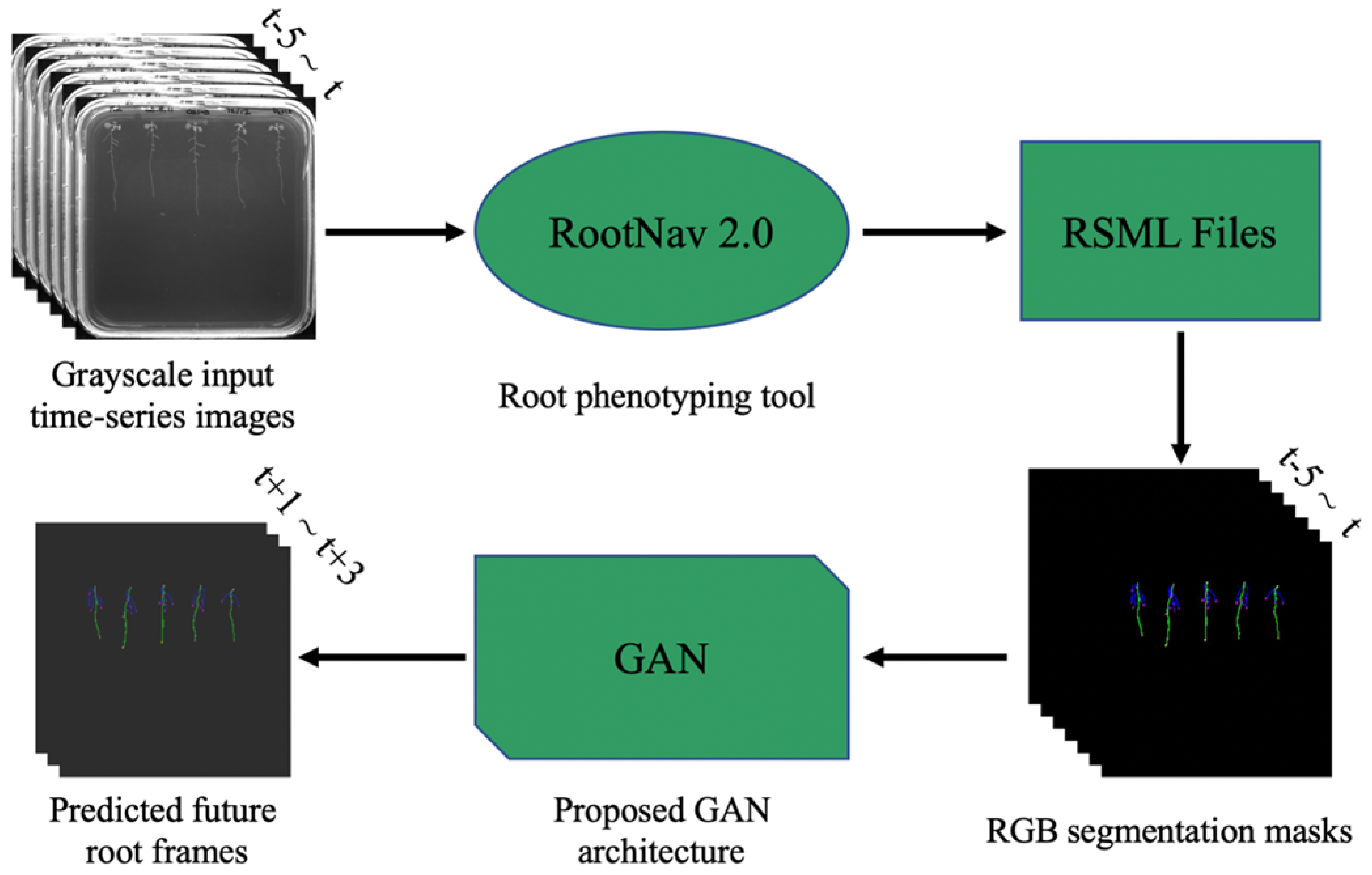
3.1. Dataset and Preprocessing
3.1.1. Brassica rapa Var. Perviridis (Komatsuna)
3.1.2. Arabidopsis thaliana
3.1.3. Preprocessing
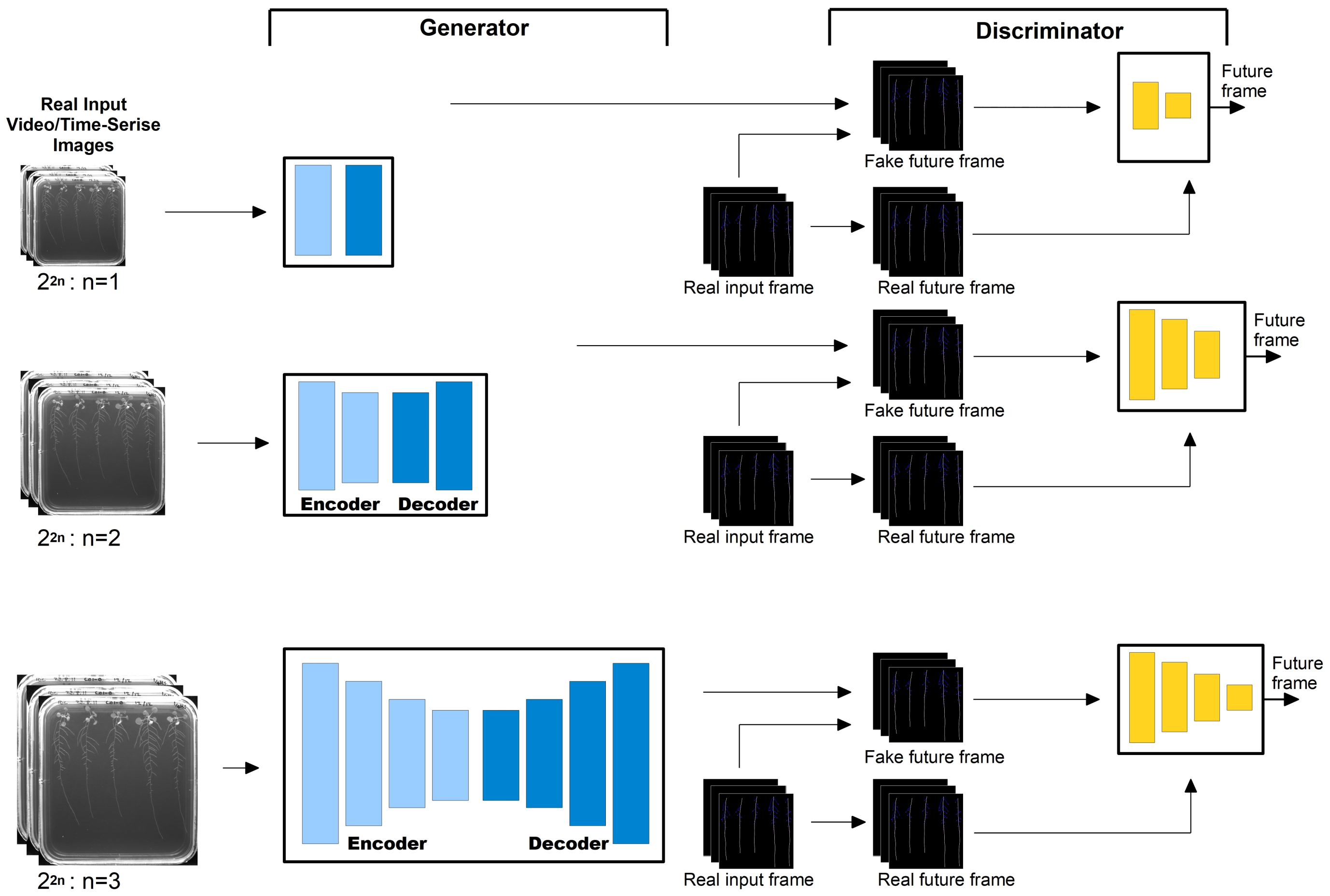
3.2. Network Design and Implementation
Proposed Architecture
3.3. Experimental Design
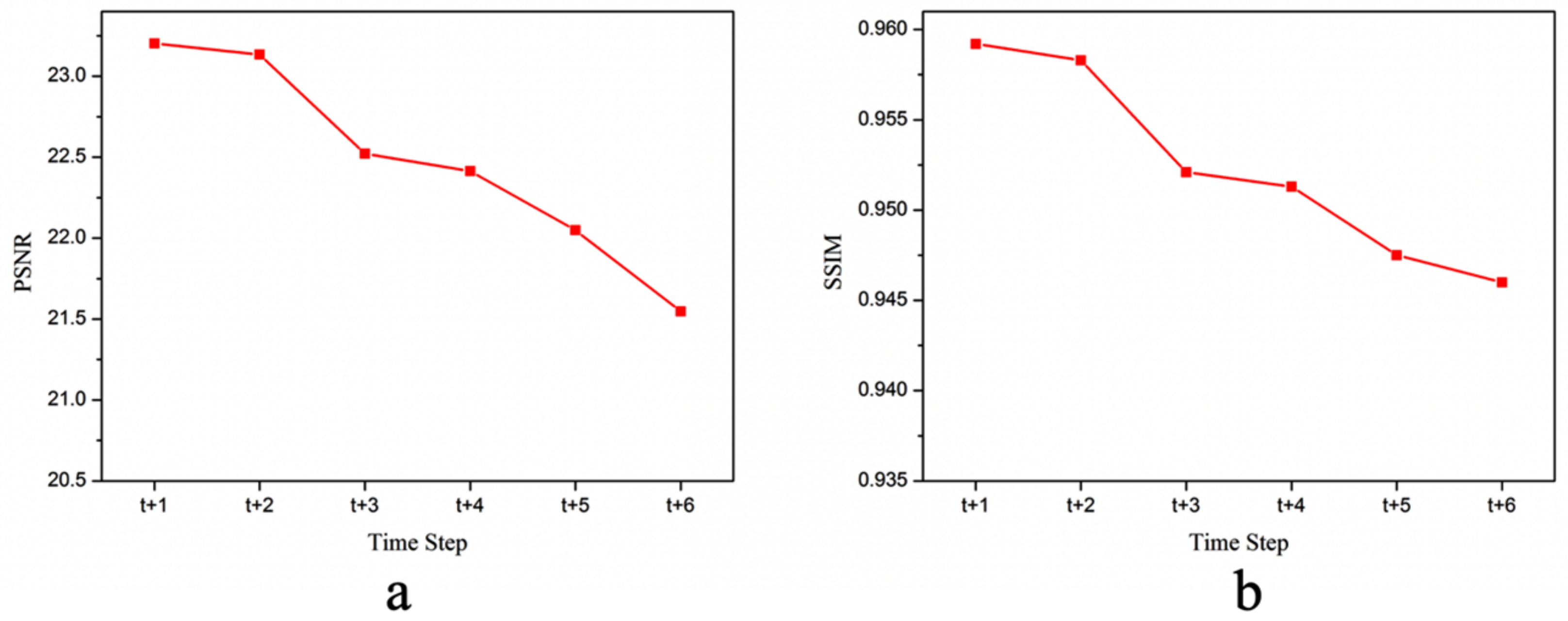
3.4. Evaluation
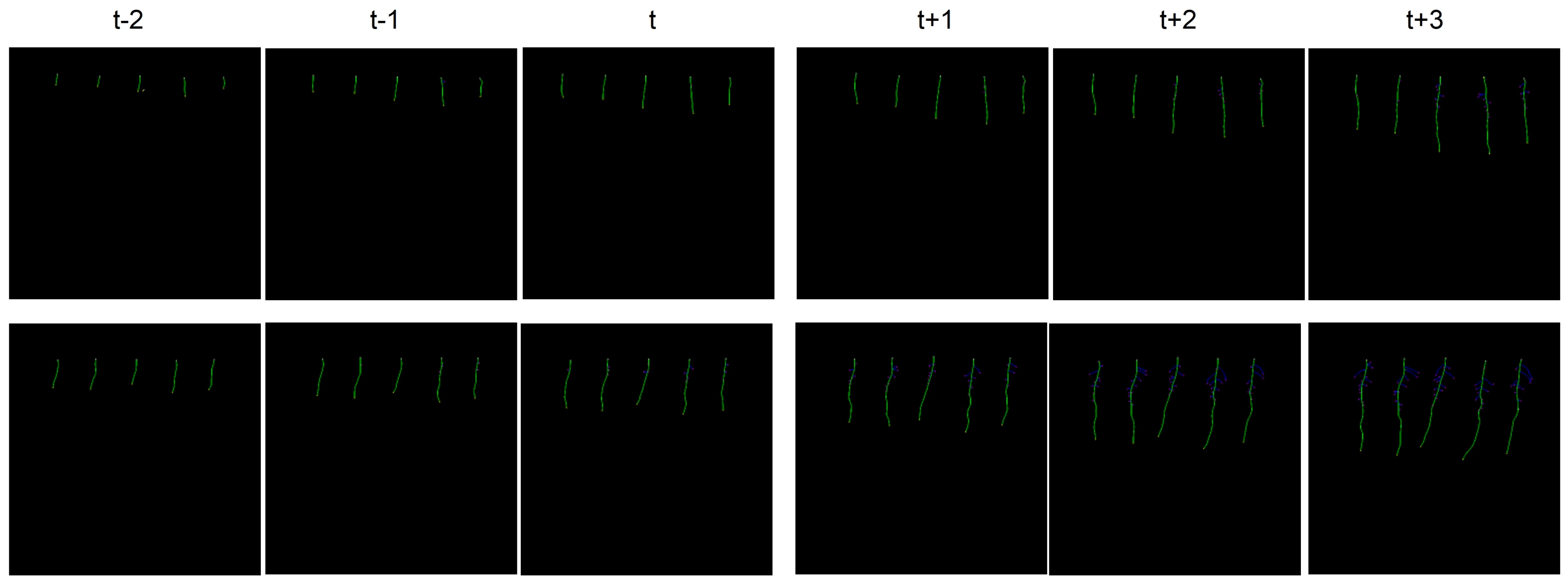
4. Results
Komatsuna Leaf Dataset
Arabidopsis thaliana Root Dataset
5. Discussion
6. Conclusions
Supplementary Materials
Author Contributions
Funding
Institutional Review Board Statement
Informed Consent Statement
Data Availability Statement
Conflicts of Interest
References
- Li, X.; Zeng, R.; Liao, H. Improving crop nutrient efficiency through root architecture modifications. J. Integr. Plant Biol. 2015, 58, 193–202. [Google Scholar] [CrossRef] [PubMed] [Green Version]
- Furbank, R.; Tester, M. Phenomics–technologies to relieve the phenotyping bottleneck. Trends Plant Sci. 2011, 16, 635–644. [Google Scholar] [CrossRef]
- Tsaftaris, S.; Minervini, M.; Scharr, H. Machine Learning for Plant Phenotyping Needs Image Processing. Trends Plant Sci. 2016, 21, 989–991. [Google Scholar] [CrossRef] [PubMed] [Green Version]
- Keller, K.; Kirchgessner, N.; Khanna, R.; Siegwart, R.; Walter, A.; Aasen, H. Soybean leaf coverage estimation with machine learning and thresholding algorithms for field phenotyping. In Proceedings of the British Machine Vision Conference, Newcastle, UK, 3–6 September 2018. [Google Scholar]
- Mochida, K.; Koda, S.; Inoue, K.; Hirayama, T.; Tanaka, S.; Nishii, R.; Melgani, F. Computer vision-based phenotyping for improvement of plant productivity: A machine learning perspective. GigaScience 2019, 8, giy153. [Google Scholar] [CrossRef] [Green Version]
- Yasrab, R.; Atkinson, J.A.; Wells, D.M.; French, A.P.; Pridmore, T.P.; Pound, M.P. RootNav 2.0: Deep learning for automatic navigation of complex plant root architectures. GigaScience 2019, 8, giz123. [Google Scholar] [CrossRef] [Green Version]
- Atkinson, J.A.; Pound, M.P.; Bennett, M.J.; Wells, D.M. Uncovering the hidden half of plants using new advances in root phenotyping. Curr. Opin. Biotechnol. 2019, 55, 1–8. [Google Scholar] [CrossRef]
- Adams, J.; Qiu, Y.; Xu, Y.; Schnable, J.C. Plant segmentation by supervised machine learning methods. Plant Phenome J. 2020, 3, e20001. [Google Scholar] [CrossRef] [Green Version]
- Darwish, A.; Ezzat, D.; Hassanien, A.E. An optimized model based on convolutional neural networks and orthogonal learning particle swarm optimization algorithm for plant diseases diagnosis. Swarm Evol. Comput. 2020, 52, 100616. [Google Scholar] [CrossRef]
- Francis, M.; Deisy, C. Disease Detection and Classification in Agricultural Plants Using Convolutional Neural Networks—A Visual Understanding. In Proceedings of the 2019 6th International Conference on Signal Processing and Integrated Networks (SPIN), Noida, India, 7–8 March 2019; pp. 1063–1068. [Google Scholar]
- Feng, X.; Zhan, Y.; Wang, Q.; Yang, X.; Yu, C.; Wang, H.; Tang, Z.; Jiang, D.; Peng, C.; He, Y. Hyperspectral imaging combined with machine learning as a tool to obtain high-throughput plant salt-stress phenotyping. Plant J. 2020, 101, 1448–1461. [Google Scholar] [CrossRef]
- Fiorani, F.; Schurr, U. Future scenarios for plant phenotyping. Annu. Rev. Plant Biol. 2013, 64, 267–291. [Google Scholar] [CrossRef] [Green Version]
- Rahaman, M.; Chen, D.; Gillani, Z.; Klukas, C.; Chen, M. Advanced phenotyping and phenotype data analysis for the study of plant growth and development. Front. Plant Sci. 2015, 6, 619. [Google Scholar] [CrossRef] [PubMed] [Green Version]
- De Vos, D.; Dzhurakhalov, A.; Stijven, S.; Klosiewicz, P.; Beemster, G.T.; Broeckhove, J. Virtual plant tissue: Building blocks for next-generation plant growth simulation. Front. Plant Sci. 2017, 8, 686. [Google Scholar] [CrossRef] [PubMed] [Green Version]
- Basu, P.; Pal, A. A new tool for analysis of root growth in the spatio-temporal continuum. New Phytol. 2012, 195, 264–274. [Google Scholar] [CrossRef]
- Chaudhury, A.; Ward, C.; Talasaz, A.; Ivanov, A.G.; Brophy, M.; Grodzinski, B.; Hüner, N.P.; Patel, R.V.; Barron, J.L. Machine vision system for 3D plant phenotyping. IEEE/ACM Trans. Comput. Biol. Bioinform. 2018, 16, 2009–2022. [Google Scholar] [CrossRef] [PubMed] [Green Version]
- Morris, E.C.; Griffiths, M.; Golebiowska, A.; Mairhofer, S.; Burr-Hersey, J.; Goh, T.; Von Wangenheim, D.; Atkinson, B.; Sturrock, C.J.; Lynch, J.P.; et al. Shaping 3D root system architecture. Curr. Biol. 2017, 27, R919–R930. [Google Scholar] [CrossRef] [Green Version]
- Alhnaity, B.; Pearson, S.; Leontidis, G.; Kollias, S. Using deep learning to predict plant growth and yield in greenhouse environments. arXiv 2019, arXiv:1907.00624. [Google Scholar]
- Elith, J. Predicting distributions of invasive species. In Invasive Species: Risk Assessment and Management; Cambridge University Press: Cambridge, UK, 2017; Volume 10. [Google Scholar]
- Goodfellow, I.; Pouget-Abadie, J.; Mirza, M.; Xu, B.; Warde-Farley, D. Generative Adversarial Nets. In Proceedings of the Advances in Neural Information Processing Systems (NIPS), Montréal, QC, Canada, 8–13 December 2014. [Google Scholar]
- Creswell, A.; White, T.; Dumoulin, V.; Arulkumaran, K.; Sengupta, B.; Bharath, A.A. Generative adversarial networks: An overview. IEEE Signal Process. Mag. 2018, 35, 53–65. [Google Scholar] [CrossRef] [Green Version]
- Valerio Giuffrida, M.; Scharr, H.; Tsaftaris, S.A. Arigan: Synthetic arabidopsis plants using generative adversarial network. In Proceedings of the IEEE International Conference on Computer Vision Workshops, Venice, Italy, 22–29 October 2017; pp. 2064–2071. [Google Scholar]
- Bhattacharjee, P.; Das, S. Temporal coherency based criteria for predicting video frames using deep multi-stage generative adversarial networks. In Proceedings of the Advances in Neural Information Processing Systems, Long Beach, CA, USA, 4–9 December 2017; pp. 4268–4277. [Google Scholar]
- Aigner, S.; Körner, M. FutureGAN: Anticipating the Future Frames of Video Sequences using Spatio-Temporal 3d Convolutions in Progressively Growing GANs. arXiv 2018, arXiv:1810.01325. [Google Scholar] [CrossRef] [Green Version]
- Danzi, D.; Briglia, N.; Petrozza, A.; Summerer, S.; Povero, G.; Stivaletta, A.; Cellini, F.; Pignone, D.; De Paola, D.; Janni, M. Can High Throughput Phenotyping Help Food Security in the Mediterranean Area? Front. Plant Sci. 2019, 10, 15. [Google Scholar] [CrossRef]
- Walter, A.; Liebisch, F.; Hund, A. Plant phenotyping: From bean weighing to image analysis. Plant Methods 2015, 11, 14. [Google Scholar] [CrossRef] [Green Version]
- Fuentes, A.; Yoon, S.; Park, D. Deep Learning-Based Phenotyping System with Glocal Description of Plant Anomalies and Symptoms. Front. Plant Sci. 2019, 10. [Google Scholar] [CrossRef] [PubMed]
- Wang, X.; Xuan, H.; Evers, B.; Shrestha, S.; Pless, R.; Poland, J. High-throughput phenotyping with deep learning gives insight into the genetic architecture of flowering time in wheat. GigaScience 2019, 8, giz120. [Google Scholar] [CrossRef] [PubMed]
- Mohanty, S.P.; Hughes, D.P.; Salathé, M. Using Deep Learning for Image-Based Plant Disease Detection. Front. Plant Sci. 2016, 7, 1419. [Google Scholar] [CrossRef] [PubMed] [Green Version]
- Akagi, D. A Primer on Deep Learning. 2017. Available online: https://www.datarobot.com/blog/a-primer-on-deep-learning/ (accessed on 14 January 2021).
- Ubbens, J.R.; Stavness, I. Deep Plant Phenomics: A Deep Learning Platform for Complex Plant Phenotyping Tasks. Front. Plant Sci. 2017, 8, 1190. [Google Scholar] [CrossRef] [PubMed] [Green Version]
- Pound, M.P.; Atkinson, J.A.; Townsend, A.J.; Wilson, M.H.; Griffiths, M.; Jackson, A.S.; Bulat, A.; Tzimiropoulos, G.; Wells, D.M.; Murchie, E.H.; et al. Deep machine learning provides state-of-the-art performance in image-based plant phenotyping. Gigascience 2017, 6, gix083. [Google Scholar] [CrossRef]
- Bah, M.D.; Hafiane, A.; Canals, R. Deep learning with unsupervised data labeling for weed detection in line crops in UAV images. Remote Sens. 2018, 10, 1690. [Google Scholar] [CrossRef] [Green Version]
- Namin, S.T.; Esmaeilzadeh, M.; Najafi, M.; Brown, T.B.; Borevitz, J.O. Deep phenotyping: Deep learning for temporal phenotype/genotype classification. Plant Methods 2018, 14, 66. [Google Scholar] [CrossRef] [Green Version]
- Sakurai, S.; Uchiyama, H.; Shimada, A.; Taniguchi, R.i. Plant growth prediction using convolutional lstm. In VISIGRAPP 2019, Proceedings of the 114th International Joint Conference on Computer Vision, Imaging and Computer Graphics Theory and Applications, Prague, Czech Republic, 25–27 February 2019; SciTePress: Setubal, Portugal, 2019; pp. 105–113. [Google Scholar]
- Zhu, Y.; Aoun, M.; Krijn, M.; Vanschoren, J.; Campus, H.T. Data Augmentation Using Conditional Generative Adversarial Networks for Leaf Counting in Arabidopsis Plants. In Proceedings of the 29th British Machine Vision Conference, Newcastle, UK, 3–6 September 2018; p. 324. [Google Scholar]
- Kuznichov, D.; Zvirin, A.; Honen, Y.; Kimmel, R. Data augmentation for leaf segmentation and counting tasks in Rosette plants. In Proceedings of the IEEE Conference on Computer Vision and Pattern Recognition Workshops, Long Beach, CA, USA, 15–21 June 2019. [Google Scholar]
- Nazki, H.; Yoon, S.; Fuentes, A.; Park, D.S. Unsupervised image translation using adversarial networks for improved plant disease recognition. Comput. Electron. Agric. 2020, 168, 105117. [Google Scholar] [CrossRef]
- Sapoukhina, N.; Samiei, S.; Rasti, P.; Rousseau, D. Data augmentation from RGB to chlorophyll fluorescence imaging Application to leaf segmentation of Arabidopsis thaliana from top view images. In Proceedings of the IEEE Conference on Computer Vision and Pattern Recognition Workshops, Long Beach, CA, USA, 15–21 June 2019. [Google Scholar]
- Uchiyama, H.; Sakurai, S.; Mishima, M.; Arita, D.; Okayasu, T.; Shimada, A.; Taniguchi, R.I. An Easy-to-Setup 3D Phenotyping Platform for KOMATSUNA Dataset. In Proceedings of the 2017 IEEE International Conference on Computer Vision Workshops (ICCVW), Venice, Italy, 22–29 October 2017; pp. 2038–2045. [Google Scholar] [CrossRef]
- Wilson, M.; Holman, T.; Sørensen, I.; Cancho-Sanchez, E.; Wells, D.; Swarup, R.; Knox, P.; Willats, W.; Ubeda-Tomás, S.; Holdsworth, M.; et al. Multi-omics analysis identifies genes mediating the extension of cell walls in the Arabidopsis thaliana root elongation zone. Front. Cell Dev. Biol. 2015, 3, 10. [Google Scholar] [CrossRef] [Green Version]
- Minervini, M.; Giuffrida, M.V.; Tsaftaris, S.A. An interactive tool for semi-automated leaf annotation. In Proceedings of the Computer Vision Problems in Plant Phenotyping (CVPPP), Swansea, UK, 7–10 September 2016. [Google Scholar]
- Wells, D.M.; French, A.P.; Naeem, A.; Ishaq, O.; Traini, R.; Hijazi, H.; Bennett, M.J.; Pridmore, T.P. Recovering the dynamics of root growth and development using novel image acquisition and analysis methods. Philos. Trans. R. Soc. B Biol. Sci. 2012, 367, 1517–1524. [Google Scholar] [CrossRef] [Green Version]
- Lobet, G.; Pound, M.; Diener, J.; Pradal, C.; Draye, X.; Godin, C.; Javaux, M.; Leitner, D.; Meunier, F.; Nacry, P.; et al. Root System Markup Language: Toward a Unified Root Architecture Description Language. Plant Physiol. 2015. [Google Scholar] [CrossRef] [PubMed]
- Goodfellow, I.; Pouget-Abadie, J.; Mirza, M.; Xu, B.; Warde-Farley, D.; Ozair, S.; Courville, A.; Bengio, Y. Generative Adversarial Nets; Curran Associates, Inc.: Red Hook, NY, USA, 2014; pp. 2672–2680. [Google Scholar]
- Karras, T.; Aila, T.; Laine, S.; Lehtinen, J. Progressive Growing of GANs for Improved Quality, Stability, and Variation. arXiv 2017, arXiv:1710.10196. [Google Scholar]
- Arjovsky, M.; Chintala, S.; Bottou, L. Wasserstein gan. arXiv 2017, arXiv:1701.07875. [Google Scholar]
- Paszke, A.; Gross, S.; Chintala, S.; Chanan, G.; Yang, E.; DeVito, Z.; Lin, Z.; Desmaison, A.; Antiga, L.; Lerer, A. Automatic differentiation in PyTorch. In Proceedings of the NIPS 2017 Autodiff Workshop, Long Beach, CA, USA, 9 December 2017. [Google Scholar]
- Xu, B.; Wang, N.; Chen, T.; Li, M. Empirical evaluation of rectified activations in convolutional network. arXiv 2015, arXiv:1505.00853. [Google Scholar]
- Odena, A.; Olah, C.; Shlens, J. Conditional Image Synthesis with Auxiliary Classifier GANs. In Proceedings of the 34th International Conference on Machine Learning, Sydney, Australia, 6–11 August 2017. [Google Scholar]
- He, K.; Zhang, X.; Ren, S.; Sun, J. Deep Residual Learning for Image Recognition. In Proceedings of the 2016 IEEE Conference on Computer Vision and Pattern Recognition (CVPR), Las Vegas, NV, USA, 27–30 June 2016; pp. 770–778. [Google Scholar] [CrossRef] [Green Version]
- Gulrajani, I.; Ahmed, F.; Arjovsky, M.; Dumoulin, V.; Courville, A. Improved Training of Wasserstein GANs. arXiv 2017, arXiv:1704.00028. [Google Scholar]
- Hore, A.; Ziou, D. Image quality metrics: PSNR vs. SSIM. In Proceedings of the 2010 20th International Conference on Pattern Recognition, Istanbul, Turkey, 23–26 August 2010; pp. 2366–2369. [Google Scholar]
- Huttenlocher, D.P.; Klanderman, G.A.; Rucklidge, W.J. Comparing images using the Hausdorff distance. IEEE Trans. Pattern Anal. Mach. Intell. 1993, 15, 850–863. [Google Scholar] [CrossRef] [Green Version]
- Dupuy, L.; Gregory, P.J.; Bengough, A.G. Root growth models: Towards a new generation of continuous approaches. J. Exp. Bot. 2010, 61, 2131–2143. [Google Scholar] [CrossRef] [Green Version]


| Generator | ||||||
|---|---|---|---|---|---|---|
| Stage | Layer | Activation | Output Dimensions | Kernel Size | Stride | Padding |
| RGB Input | Conv | LeakyReLU | 3 × 128 | 1 × 1 × 1 | 1 × 1 × 1 | |
| 128 × 128–64 × 64 | Conv | LeakyReLU | 128 × 128 | 3 × 3 × 3 | 1 × 1 × 1 | 1 × 1 × 1 |
| Conv | LeakyReLU | 128 × 526 | 1 × 2 × 2 | 1 × 2 × 2 | ||
| 64 × 64–32 × 32 | Conv | LeakyReLU | 256 × 256 | 3 × 3 × 3 | 1 × 1 × 1 | 1 × 1 × 1 |
| Conv | LeakyReLU | 256 × 512 | 1 × 2 × 2 | 1 × 2 × 2 | ||
| 32 × 32–16 × 16 | Conv | LeakyReLU | 512 × 512 | 3 × 3 × 3 | 1 × 1 × 1 | 1 × 1 × 1 |
| Conv | LeakyReLU | 512 × 512 | 1 × 2 × 2 | 1 × 2 × 2 | ||
| 16 × 16–8 × 8 | Conv | LeakyReLU | 512 × 512 | 3 × 3 × 3 | 1 × 1 × 1 | 1 × 1 × 1 |
| Conv | LeakyReLU | 512 × 512 | 1 × 2 × 2 | 1 × 2 × 2 | ||
| 8 × 8–4 × 4 | Conv | LeakyReLU | 512 × 512 | 3 × 3 × 3 | 1 × 1 × 1 | 1 × 1 × 1 |
| Conv | LeakyReLU | 512 × 512 | 1 × 2 × 2 | 1 × 2 × 2 | ||
| Middle Block | Conv | LeakyReLU | 512 × 512 | 3 × 3 × 3 | 1 × 1 × 1 | 1 × 1 × 1 |
| Conv | LeakyReLU | 512 × 512 | 6 × 1 × 1 | 1 × 1 × 1 | ||
| Conv Trans | LeakyReLU | 512 × 512 | 6 × 1 × 1 | 1 × 1 × 1 | ||
| Conv | LeakyReLU | 512 × 512 | 3 × 3 × 3 | 1 × 1 × 1 | 1 × 1 × 1 | |
| Discriminator | ||||||
| 4 × 4–8 × 8 | Conv Trans | LeakyReLU | 512 × 512 | 1 × 2 × 2 | 1 × 2 × 2 | |
| Conv | LeakyReLU | 512 × 512 | 3 × 3 × 3 | 1 × 1 × 1 | 1 × 1 × 1 | |
| 8 × 8–16 × 16 | Conv Trans | LeakyReLU | 512 × 512 | 1 × 2 × 2 | 1 × 2 × 2 | |
| Conv | LeakyReLU | 512 × 512 | 3 × 3 × 3 | 1 × 1 × 1 | 1 × 1 × 1 | |
| 16 × 16–32 × 32 | Conv Trans | LeakyReLU | 512 × 512 | 1 × 2 × 2 | 1 × 2 × 2 | |
| Conv | LeakyReLU | 512 × 512 | 3 × 3 × 3 | 1 × 1 × 1 | 1 × 1 × 1 | |
| 32 × 32–64 × 64 | Conv Trans | LeakyReLU | 512 × 256 | 1 × 2 × 2 | 1 × 2 × 2 | |
| Conv | LeakyReLU | 256 × 256 | 3 × 3 × 3 | 1 × 1 × 1 | 1 × 1 × 1 | |
| Conv Trans | LeakyReLU | 526 × 128 | 1 × 2 × 2 | 1 × 2 × 2 | ||
| Conv | LeakyReLU | 128 × 128 | 3 × 3 × 3 | 1 × 1 × 1 | 1 × 1 × 1 | |
| RGB Output | Conv | 128 × 3 | 1 × 1 × 1 | 1 × 1 × 1 | ||
| t + 1 | t + 2 | t + 3 | t + 4 | t + 5 | t + 6 | |
|---|---|---|---|---|---|---|
| PSNR | 23.2017 | 23.1346 | 22.5215 | 22.4145 | 22.0487 | 21.5475 |
| SSIM | 0.9592 | 0.9583 | 0.9521 | 0.9513 | 0.9475 | 0.9460 |
| t + 1 | t + 2 | t + 3 | |
|---|---|---|---|
| IoUbg | 0.9982 | 0.9975 | 0.9966 |
| IoUroot | 0.5396 | 0.5528 | 0.5587 |
| mIoUroot | 0.7689 | 0.7751 | 0.7776 |
Publisher’s Note: MDPI stays neutral with regard to jurisdictional claims in published maps and institutional affiliations. | |
Sample Availability: Samples of the compounds are available from the authors. |
© 2021 by the authors. Licensee MDPI, Basel, Switzerland. This article is an open access article distributed under the terms and conditions of the Creative Commons Attribution (CC BY) license (http://creativecommons.org/licenses/by/4.0/).
Share and Cite
Yasrab, R.; Zhang, J.; Smyth, P.; Pound, M.P. Predicting Plant Growth from Time-Series Data Using Deep Learning. Remote Sens. 2021, 13, 331. https://doi.org/10.3390/rs13030331
Yasrab R, Zhang J, Smyth P, Pound MP. Predicting Plant Growth from Time-Series Data Using Deep Learning. Remote Sensing. 2021; 13(3):331. https://doi.org/10.3390/rs13030331
Chicago/Turabian StyleYasrab, Robail, Jincheng Zhang, Polina Smyth, and Michael P. Pound. 2021. "Predicting Plant Growth from Time-Series Data Using Deep Learning" Remote Sensing 13, no. 3: 331. https://doi.org/10.3390/rs13030331
APA StyleYasrab, R., Zhang, J., Smyth, P., & Pound, M. P. (2021). Predicting Plant Growth from Time-Series Data Using Deep Learning. Remote Sensing, 13(3), 331. https://doi.org/10.3390/rs13030331