Assessing the Potential of Geostationary Himawari-8 for Mapping Surface Total Suspended Solids and Its Diurnal Changes

Abstract

Ocean color sensors, typically installed on polar-orbiting satellites, have been used to monitor oceanic processes for last three decades. However, their temporal resolution is not considered to be adequate for monitoring highly dynamic oceanic processes, especially when considering data gaps due to cloud contamination. The Advanced Himawari Imager (AHI) onboard the Himawari-8, a geostationary satellite operated by the Japan Meteorological Agency (JMA), acquires imagery every 10 min at 500 m to 2000 m spatial resolution. The AHI sensor with three visible, one near-infrared (NIR), and two shortwave-infrared (SWIR) bands displays good potential in monitoring oceanic processes at high temporal resolution. This study investigated and identified an appropriate atmospheric correction method for AHI data; developed a model for Total Suspended Solids (TSS) concentrations estimation using hyperspectral data and in-situ measurements of TSS; validated the model; and assessed its potential to capture diurnal changes using AHI imagery. Two image-based atmospheric correction methods, the NIR-SWIR method and the SWIR method were tested for correcting the AHI data. Then, the new model was applied to the atmospherically corrected AHI data to map TSS and its diurnal changes in the Pearl River Estuary (PRE) and neighboring coastal areas. The results indicated that the SWIR method outperformed the NIR-SWIR method, when compared to in-situ water-leaving reflectance data. The results showed a good agreement between the AHI-derived TSS and in-situ measured data with a coefficient of determination (R²) of 0.85, mean absolute error (MAE) of 3.1 mg/L, a root mean square error (RMSE) of 3.9 mg/L, and average percentage difference (APD) of 30% (TSS range 1–40 mg/L). Moreover, the diurnal variation in the turbidity front, using the Normalized Suspended Material Index (NSMI), showed the capability of AHI data to track diurnal variation in turbidity fronts, due to high TSS concentrations at high temporal frequency. The present study indicates that AHI data with high image capturing frequency can be used to map surface TSS concentrations. These TSS measurements at high frequency are not only important for monitoring the sensitive coastal areas but also for scientific understanding of the spatial and temporal variation of TSS.

1. Introduction

Ocean color satellites in low altitude polar orbits contribute to the effective monitoring of the dynamic status of oceans, coasts, and inland water resources [1,2,3]. Other polar-orbiting satellites designed for terrestrial applications also contributed to the ocean color applications, but some limitations are observed [4]. Monitoring of the Total Suspended Solids (TSS) or Total Suspended Matter (TSM) concentrations for water quality application commenced with the widely used historic ocean color sensors, such as Coastal Zone Color Scanner (CZCS) [5], Sea-Viewing Wide Field-of-view Sensor (SeaWiFS) [2,6], and the MEdium Resolution Imaging Spectrometer (MERIS) [7,8,9]. Many studies successfully retrieved a wide range of TSS with the MODerate Resolution Imaging Spectrometer (MODIS), onboard the Terra and Aqua satellites [8,10,11,12]. Although each MODIS sensor completed its planned life span, it is expected to beam down the data beyond 2020 [13]. The Land and Ocean Color Instrument (OLCI) onboard Sentinel-3 A, launched by the European Space Agency (ESA) in February 2016 also demonstrated the potential for mapping the TSS dynamics in coastal waters [3,14]. Another OLCI sensor onboard Sentinel-3 B recently joined its twin in April 2018. Landsat sensors from the historic Landsat Multispectral Scanner (MSS) to the latest Operational Land Imager (OLI) were also widely used in the observation of TSS concentrations in coastal environments [1,15,16,17,18]. The Multi Spectral Instrument (MSI) onboard the Sentinel-2 mission, with a temporal resolution of 5 days with twin satellites Sentinel-2 A and Sentinel-2 B, also demonstrated significant results for mapping TSS at 20-m spatial resolution [19,20,21]. Free satellite data available from low earth-orbiting satellite sensors, such as MSI, OLI, OLCI, and MODIS, display adequate spatial resolutions from 10–20 m, 30 m, 300 m, and 250–1000 m, respectively. Although the temporal resolutions of MODIS, OLCI, MSI, and OLI sensors, are generally ∼1–2 days, ∼2–3 days, ∼5 days, and ∼16 days, respectively. With these datasets, it is inadequate to monitor diurnal variations in TSS, although they can still be used to monitor TSS variations at particular time instants for the coastal and open ocean waters during the cloud-free periods [22]. These sensors cannot capture the high-frequency changes occurring in the estuaries and coastal areas, as a result of repeated vertical resuspension and horizontal advection, subject to the impact of tidal and wind-driven currents. Thompson, et al. [23] reported that resuspension solely due to tidal currents can vary from 8% to nearly 13% for a small period (< 30 min). Therefore, to better understand the estuarine or coastal processes, it is important to monitor diurnal variability in TSS concentrations. Satellite sensors capable of capturing several images per day, presently offered only by geostationary satellite sensors, can be used to monitor these variations. In addition, recent studies of geostationary satellite sensors show that high temporal changes in the coastal processes can be well attained with a high temporal resolution of these sensors, under varying atmospheric conditions. These studies relied on various sensors including (1) the Spinning Enhanced Visible and InfraRed Imager (SEVIRI) onboard the European Union’s METeorological SATellite for monitoring TSS [22], Turbidity, and the light attenuation coefficient [24]; (2) the Geostationary Ocean Color Imager (GOCI) onboard the Communication, Ocean and Meteorological Satellite (COMS) from South Korea for monitoring TSS [25], turbidity fronts [26], water transparency [27], harmful algal blooms [28], and diurnal variability in cyanobacteria [29]; and (3) Advanced Himawari Imager (AHI), onboard Himawari-8, launched by the Japan Aerospace Exploration Agency (JAXA) to monitor ocean color [30] and high-frequency changes in floating algae [31] (please refer to Table S1 for a brief description on the significant characteristics of these geostationary sensors). Geostationary satellites also have some limitations in terms of mapping coastal dynamics. For example, SEVIRI applications are limited to the mapping of TSS at 3.0 × 6.5 km spatial resolution, and the shortwave infrared (SWIR) bands required for high-quality atmospheric correction over highly turbid coastal waters are absent in the present and planned GOCI sensors [32]. The coverage area of GOCI is also limited.

This study examines the potential of the AHI sensor for monitoring the coastal surface TSS, as the AHI sensor is deployed with suitable wavebands of visible, Near Infrared (NIR) and Shortwave Infrared (SWIR), and high temporal resolution (every 10 min). The Pearl River Estuary (PRE) and neighboring coastal waters were selected, showing relatively strong daily sedimentary and runoff variations [33]. Additionally, the marine ecosystem adjacent to the PRE is disturbed by the problem of sediment and effluent runoff from rapid industrial and urban development [34]; high-frequency mapping of TSS is, thus, critical for monitoring the coastal ecosystem. This study required (i) implementing atmospheric correction methods for AHI data, using two separate atmospheric correction approaches i.e., the NIR-SWIR method (based on the NIR and SWIR-I bands) and the SWIR method (based on the SWIR-I and SWIR-II bands), (ii) developing a new AHI-based TSS model using in-situ radiometric and TSS measurements, (iii) cross-validating to evaluate the capability of the new model to monitor TSS using the atmospherically corrected AHI data; and (iv) monitoring diurnal TSS changes and turbidity fronts based on the Normalized Suspended Material Index (NSMI) method over the PRE and the neighboring coastal waters.

2. Materials and Methods

2.1. Study Area

The study area comprises the Pearl River Estuary (PRE) along with the areas farther along the coast, in the east and west directions (Figure 1). The Pearl River (Chinese name Zhujiang River), which is 2216 km in length, is the longest river in Southern China and the third-longest river in China, with a catchment area of 453,000 km². Its mean annual runoff, which is 300 billion m³, ranks 2nd in Chinese rivers and is next only to the Yangtze River [35]. The dry season lasts from October to April and the downstream annual discharge fluctuates significantly, depending on the total rainfall received in the upstream catchment. Relatively low rainfall, which is approximately 30–40 mm/month, and its discharge into the PRE, are typically around 1500 m³/s during the dry season [35]. During the wet season, from May to September, the southwest monsoon brings warm, humid air from the lower latitudes, causing high rainfall (300–400 mm/month), where the flows can reach up to 20,000 m³/s. The annual discharge of suspended sediments reaches 87 million tons, among which more than 90% are discharged during the wet season [36]. In the northwestern estuary, the TSS concentration is as high as 100 mg/L during the wet season [37]. The Pearl and Huangmao River estuaries play an important role in transportation, fisheries, and aquaculture, and they are also the habitats of rare marine species such as the Chinese White Dolphin. The development of industries and urbanization in Guangdong during the last 30 years caused serious environmental degradation, and reduced water quality along its coastline and in the PRE [38]. Eutrophication is the most serious environmental issue in the PRE. It caused frequent red tide and harmful algal bloom events in the estuary and its neighboring coastal waters, since the 1980s, along with significant economic losses [39]. The high concentrations of suspended sediments, red tides, and dissolved material affects the optical properties of the estuarine waters, which make these waters challenging to the application of ocean color remote sensing, for the determination of dissolved and solid components. Since the nutrients responsible for eutrophication mostly originate from discharged runoff and their concentrations are higher in the surface layer than at the bottom, they can be detected through Ocean Color Remote Sensing and possible sources can be identified. Environment protection agencies and local communities have great concerns with the water quality in the PRE and the neighboring coastal areas, and the programs designed to improve the water quality are under implementation. Therefore, remote sensing techniques have potential values for such recovery programs, by providing dynamic and up-to-date data of TSS.

2.2. Overview of Himawari-8AHI

Himawari-8 is a geostationary meteorological satellite placed at 140.7 °E above the equator, covering the East Asian and Western Pacific regions. It is operated by the Japan Meteorological Agency (JMA). However, it was launched by JAXA in October 2014, and from July 2015 it became completely operational [30]. AHI, the primary sensor of Himawari-8, has 16 spectral bands to observe the earth systems; three visible channels (0.43–0.48, 0.50–0.52, and 0.63–0.66 μm), one NIR (0.85–0.87 μm), two SWIR channels (1.60–1.62 and 2.25–2.27 μm), and 10 thermal infrared (TIR) channels (∼3.7–13.4 μm) [40]. The instantaneous field of view (IFOV) of blue, green, and NIR channels at the sub-satellite point (SSP) is 1 km, whereas the red channel captures at 0.5 km. The IFOV of the SWIR and TIR channels is 2 km.

Table 1. Specifications of the first six bands of the Himawari-8 AHI sensor.

Band Number	Central Wavelength (μm)	Spatial Resolution at SSP * (km)
1	0.47	1
2	0.51	1
3	0.64	0.5
4	0.86	1
5	1.6	2
6	2.3	2

* SSP is the sub-satellite point.

shows the specifications of the first six bands of AHI used in this study. The temporal resolution of Himawari-8 varies depending on different sample regions—the full earth disk, two landmark areas, and three target areas [41]. The temporal resolution for capturing the full earth disk and two target areas (Regions-1 and 2 over Japan) is fixed, every 10 min and every 2.5 min, respectively. However, for the two landmark areas and one target area (Region-3), the scanning frequency is flexible (from 0.5–2.5 min), to enable prompt reaction to meteorological conditions [41].

2.3. Satellite Data Used and Atmospheric Correction Approaches

2.3.1. Satellite Data

The AHI Himawari level 1 Gridded data (NetCDF4 format) of the study area were obtained from JAXA’s Himawari P-Tree system. Using the P-Tree system, the cloud cover extent could also be assessed visually, prior to downloading the data. Images at every 10 min interval, from 10:00 to 15:00 HKT, were acquired during the winter season (December, January, February) from 2016 to 2019 (

Table 2. AHI data used in this study.

Date	Time	Timestep
25 January 2016	10:00–15:00	every 10 min
7 February 2016	10:00–15:00	every 10 min
8 February 2016	10:00–15:00	every 10 min
19 December 2016	10:00–15:00	every 10 min
27 January 2017	10:00–15:00	every 10 min
11 January 2018	10:00–15:00	every 10 min
12 January 2018	10:00–15:00	every 10 min
16 January 2018	10:00–15:00	every 10 min
23 January 2019	10:00–15:00	every 10 min

). The data for cloud-free clear days in winter months were selected, as sun-glint is substantial over the study area during the afternoon in summer months.

2.3.2. AHI Water-Leaving Reflectance Processing

Cloud free images of three visible, one NIR, and two SWIR bands were used. All bands were aggregated to a uniform spatial resolution of 2 km by the JAXA [42]. The albedo of these bands was converted to the top of atmosphere reflectance (${\rho }_{toa}$) by diving the albedo with the solar zenith angle (${\theta }_0$), using Equation (1). Full disk data were clipped to the study area, to expedite processing.

$${\rho }_{toa }\left(\lambda \right)=\frac{Albedo \left(\lambda \right)}{Cos{\theta }_0}$$

(1)

where $Albedo$ is the recorded albedo in the respective band $\left(\lambda \right)$. The ${\rho }_{toa}\left(\lambda \right)$ can be divided into the following components, as shown in Equation (2), to understand the atmospheric contributions in ${\rho }_{toa}\left(\lambda \right)$ [22,43]. For notational simplicity, the $\left(\lambda \right)$ notation is dropped hereafter.

$${\rho }_{toa}={\rho }_a+{\rho }_r+{\rho }_{ra}+{\rho }_g+T_v{T}_0\left({\rho }_{wc}+{\rho }_w\right)$$

(2)

where ${\rho }_a$ is aerosols scattering reflectance, ${\rho }_r$ is Rayleigh scattering reflectance by air molecules, and ${\rho }_{ra}$ is the contribution due to coupling between air molecules and aerosols. Usually, ${\rho }_{ra}$ is incorporated into the ${\rho }_a$ calculations, so it can be omitted in Equation (2). The contribution of sun-glint is represented by ${\rho }_g , T_v$ and $T_0$ are total diffuse transmittance along the viewing direction and incident direction, ${\rho }_{wc}$ is reflectance that occurred as a result of white caps, and ${\rho }_w$ is the water-leaving reflectance of the water surface. ${\rho }_g$is substantial only if the relative azimuth angle ($\Delta \phi =\left|\mathrm{solar} \mathrm{azimuth} ({\phi }_0)-\mathrm{satellite} \mathrm{azimuth} \left({\phi }_v\right)\right|$) is near 180° and the satellite zenith angle (${\theta }_v$) is near ${\theta }_0$ [43]. For this study region, from May to August on/after 14:00 HKT, ${\rho }_g$is substantial (Figure S1 of Supplementary data) as ${\theta }_v$ is close to ${\theta }_0$and $\Delta \phi =\left|{\phi }_0-{\phi }_v\right|$ is close to 180°, for these months. Therefore, in this study, only cloud-free images captured from 10 a.m. to 3 p.m. in winter are investigated. For all images captured for the study region, the ${\theta }_v$ranges from 38 to 42° and ${\phi }_v$ ranges from 3° to 54° and from 246° to 295° during 10:00–12:30 and 13:00–16:00 HKT (UTC + 8 h), respectively. Therefore, ${\rho }_g$ was considered to be insignificant in Equation (2). Moreover, ${\rho }_{wc}$ for the study area was also considered to be insignificant, as the wind speed was less than 10 m s⁻¹ on the dates considered in this study, as the ${\rho }_{wc}$ should be considered during the atmospheric correction only when the wind speed is higher than 10 ms⁻¹ [44]. Hence, after considering the insignificant influences of sun-glint reflectance and white caps reflectance, Equation (2) could be reduced as:

$${\rho }_{toa}={\rho }_a+{\rho }_r+T_0{T}_v{\rho }_w$$

(3)

The Rayleigh corrected reflectance (${\rho }_{Re}$) could be calculated if ${\rho }_r$ is known a priori, as shown in Equation (4)

$${\rho }_{Re}={\rho }_{toa}-{\rho }_r={\rho }_a+T_0{T}_v{\rho }_w$$

(4)

${\rho }_r$, $T_0$and $T_v$are the unknown parameters in Equation (4) and these were produced as a look-up-table (LUT) utilizing the 6SV v1.1 [45] for the first six AHI bands, using the parameters shown in Table S2. 6S was modified for AHI by applying the spectral response function (SRF) of all AHI bands in the original 6S model. While generating LUT, the values of satellite geometry, ${\theta }_v$and ${\phi }_v$, were kept constant at 40.1° and 127.5°, respectively; these were the average values of ${\theta }_v \mathrm{and} {\phi }_v$ for the study area. Additionally, both ${\theta }_v$ and ${\phi }_v$ varied by only ∼2° for the entire study area. As the Solar Zenith angle (${\theta }_o$) and Solar Azimuth angle (${\phi }_o$) vary during the day; the values were obtained from the image metadata file. Only the water vapor and the ozone concentration vary in the atmospheric model, as these two quantities are proven to show higher temporal and spatial inconsistency than other gases, which are believed to be fairly mixed in both the temporal and spatial scales [46]. The ozone Total Column (DOAS) data product (OMDOAO3e v003) and Aerosol Optical Depth 550 nm: Dark Target (MOD08_D3 v6.1) were obtained from Giovanni [47]. The water vapor content, high in the NIR, was considered based on the total precipitous water vapor content (PWC). PWC was quite variable throughout the day, so the hourly values were obtained from the MERRA-2 Model M2T1NXSLV v5.12.4 (Table S3). In addition, a tropical aerosol model acted as the aerosol model needed in 6SV v1.1. AHI SWIR band 5, with a threshold of ${\rho }_{Re}^5$ > 0.0215, was used for the land and cloud masking in this study, as this band is proven to be efficient in differentiating land, cloud, and floating objects from the water pixels, even in extremely turbid waters [48].

The aerosol, ${\rho }_a$, correction in Equation (4) was achieved by two different aerosol reflectance assessment approaches—(1) NIR-SWIR and (2) SWIR. In the NIR-SWIR method, one NIR band (860 nm: band 4 of AHI) and one SWIR band (1609 nm: band 5 of AHI) were used, whereas SWIR band 5 and SWIR band 6 (2257 nm) were used when the SWIR method was adopted. In the SWIR bands, the absorption by water surface was high and ${\rho }_w$ was negligible in the SWIR bands, even for the high turbid water types [4,49]. In turbid waters, ${\rho }_w$ in the NIR band was significant. However, in the case of clearwater, pixels ${\rho }_w$ could be assumed to be nearly zero, even in the NIR bands. With ${\rho }_w$ = 0 in band 4, 5, and 6, Equation (4) could be rewritten for these bands as follows:

$${\rho }_{Re}^4={\rho }_{toa}^4-{\rho }_r^4={\rho }_a^4; {\rho }_{Re}^5={\rho }_{toa}^5-{\rho }_r^5={\rho }_a^5; \mathrm{and} {\rho }_{Re}^6={\rho }_{toa}^6-{\rho }_r^6={\rho }_a^6$$

(5)

In the above-mentioned atmospheric correction methods, the aerosol reflectance ratio (ε), ${\epsilon }^{\left(4,5\right)}$ for AHI bands 4, 5, and ${\epsilon }^{\left(5,6\right)}$ for AHI band 5, 6 was needed, and could be calculated by Equation (6), as given below:

$${\epsilon }^{\left(4,5\right)}=\frac{{\rho }_a^4}{{\rho }_a^5}=\frac{{\rho }_c^4}{{\rho }_c^5}; \mathrm{and} {\epsilon }^{\left(5,6\right)}=\frac{{\rho }_a^5}{{\rho }_a^6}=\frac{{\rho }_c^5}{{\rho }_c^6}$$

(6)

Aerosol reflectance ratios ${\epsilon }^{\left(4,5\right)}$ and ${\epsilon }^{\left(5,6\right)}$were calculated for every image above the clear seawater area (box C in Figure 1) by applying Equation (6). The location and dimension of box A and box C varied constantly, due to the cloud cover. The distribution of ε was found to be normal (Figure 2), hence it was assumed that the ε was spatially consistent for the study area, the median values of ${\epsilon }^{\left(4,5\right)}$ and ${\epsilon }^{\left(5,6\right)},$ calculated from every scene, were used to correct AHI data. Moreover, one standard deviation (STD) of corresponding ${\epsilon }^{\left(4,5\right)}$ and ${\epsilon }^{\left(5,6\right)}$ values were considered as the ambiguities in the aerosol reflectance ratio. The value of ${\epsilon }^{\left(4,5\right)}$ and ${\epsilon }^{\left(5,6\right)}$ was 1.96 ± 0.145 and 1.72 ± 0.142, considering all available AHI data.

By replacing ${\rho }_a$ with ${\rho }_a^4$ and ${\rho }_a^5$ for band 4 and band 5 for the NIR-SWIR and SWIR method, Equations (4) and (6) could be combined to calculate the atmospherically corrected ${\rho }_w^4$and ${\rho }_w^5$, as follows:

$${\rho }_w^4=\frac{{\rho }_{Re}^4-p_a^4}{T_0^4{T}_v^4}=\frac{{\rho }_{Re}^4-{\epsilon }^{\left(4,5\right)}{p}_a^5}{T_0^4{T}_v^4}$$

(7)

$${\rho }_w^5=\frac{{\rho }_{Re}^5-p_a^5}{T_0^5{T}_v^5}=\frac{{\rho }_{Re}^4-{\epsilon }^{\left(5,6\right)}{p}_a^6}{T_0^5{T}_v^5}$$

(8)

In both atmospheric correction methods, ${\rho }_w^i$ (i = other bands) could be calculated using Equations (9) and (10), with the known reflectance from aerosols in longer wavelengths (${\rho }_a^5$ and ${\rho }_a^6$).

$$NIR-SWIR: {\rho }_w^i=\frac{{\rho }_{Re}^i-{\epsilon }^{\left(i,5\right)}{p}_a^5}{T_0^i{T}_v^i}$$

(9)

$$SWIR: {\rho }_w^i=\frac{{\rho }_{Re}^i-{\epsilon }^{\left(i,6\right)}{p}_a^6}{T_0^i{T}_v^i}$$

(10)

where ${\epsilon }^{\left(i,5\right)}$ and ${\epsilon }^{\left(i,6\right)}$could be obtained through exponential extrapolation [50], as follows:

$${\epsilon }^{\left(i,5\right)}={\left({\epsilon }^{\left(4,5\right)}\right)}^{\delta i}; \delta i=\frac{{\lambda }_5-{\lambda }_i}{{\lambda }_5-{\lambda }_4}$$

(11)

$${\epsilon }^{\left(i,6\right)}={\left({\epsilon }^{\left(5,6\right)}\right)}^{\delta i}; \delta i=\frac{{\lambda }_6-{\lambda }_i}{{\lambda }_6-{\lambda }_5}$$

(12)

2.4. In-Situ Hyperspectral Data

Two field datasets were used in this study. Radiometric measurements were collected using the ASD FieldSpec Spectroradiometer, during the cruise surveys in August 2014. Whereas the TriOS RAMSES Spectroradiometer were used during the cruise surveys conducted in January and May 2018, and January 2019. Water samples were collected simultaneously during all field campaigns and analyzed in the laboratory, using the standard methods explained in Section 2.5.

2.4.1. ASD FieldSpec Spectroradiometer Data

Radiometric measurements were carried out at seventeen stations in the PRE during 8–15 August 2014 (green dots, shown in Figure 1). ASD FieldSpec Spectroradiometer with a spectral range of 350 to 1050 nm (1-nm resolution) was used to measure the above-water upwelling radiance ($L_w$), using the National Aeronautics and Space Administration U.S. (NASA) protocol [51]. To limit the boat shadow and sun-glint effects, the radiometric sensor was mounted at an azimuth angle of 135° to the plane of incident radiation. The total upwelling radiance from the water surface ($L_{up}$) was measured at 40° from the zenith direction. Skylight radiance ($L_{sky}$) was measured with the radiometer looking upward. The downwelling irradiance, $E_d$ (0⁺), was calculated using measurements of radiance from a 30% reflecting gray reference ($L_p$), with a known calibration coefficient (ρ):

$$E_d(0^{+})=\pi L_{p/\rho }$$

(13)

2.4.2. TriOS RAMSES Spectroradiometer Data

During field campaigns in January and May 2018, and January 2019, TRiOS RAMSES Spectroradiometers were used with a spectral range of 320–950 nm (3.3-nm resolution). In total, thirty-seven measurements were collected in the coastal waters of Hong Kong during these field campaigns (red and pink dots in Figure 1). Three inter-calibrated radiometers, one ACC for irradiance, and two ARC for radiances, were used to measure $L_{up}$, $L_{sky}, \mathrm{and} E_d$ (0⁺). The sensor view followed the mounting description of Ruddick, et al. [52]. The sensors were mounted such as the relative azimuth angle between $L_{up}$ and $L_{sky}$ with reference to sun it was 135°, and $L_{up}$ was detected at a zenith angle of 45° from nadir. $E_d$ (0⁺) was also measured on-site in this case. All radiometers operated simultaneously, and ten measurements were collected for every station and averaged, after filtering out the noisy data. Moreover, measurements were collected within a 4-h interval (10:00 a.m.–2:00 p.m.) to avoid the potential impact of sun-glint at low sun angles. The remote-sensing reflectance ($R_{rs}$) was calculated at each sampling station as:

$$R_{rs}=L_w/E_d(0^{+})$$

(14)

$$L_w= L_{up}-r L_{sky}$$

(15)

where r is the air–water interface reflection coefficient, generally varying from 0.022 and 0.028 [53]. We calculated the r values using HydroLight, with an average of 0.026 (±0.003) for the PRE. In-situ $R_{rs}$spectra were weighted by spectral response functions SRF(λ) of AHI bands, thus, deriving a multi-spectral data comparable to atmospherically corrected AHI-reflectance from image as:

$$R_{rs, \left(situ\right)}\left({\lambda }_i\right)=\frac{{\int }_k^{ }{R}_{rs\ast }\left(\lambda \right)\times SRF \left(\lambda \right)d\lambda }{{\int }_k^{ }SRF \left(\lambda \right)d\lambda }$$

(16)

where $R_{rs, \left(situ\right)}\left({\lambda }_i\right)$ is the AHI reflectance simulated from in-situ reflectance, k is the bandwidth (nm), ${\lambda }_i$is the central wavelength of spectral band, i is the number of AHI spectral band, and SRF is the spectral response function of AHI applied to the in-situ hyperspectral remote-sensing reflectance. Figure 3a,b shows the remote-sensing reflectance data collected during August 2014 and May 2018, January 2018 and 2019, respectively.

As the AHI data was available after September 2015, data collected only on 11 January 2018, and 23 January 2019 was used as a validation dataset for validating the AHI-derived water-leaving reflectance. Data collected during May 2018 was not considered due to the land adjacency problem and low spatial resolution of AHI. To obtain the match-up data corresponding to the AHI datasets, we selected the $R_{rs, \left(situ\right)}$ data within ±5 min, w.r.t AHI overpass. In total, we selected 16 TriOS and AHI-derived matchup pairs to cross-validate the AHI-derived $R_{rs}$. Atmospherically corrected AHI water leaving reflectance (${\rho }_w$) in the visible bands were converted to AHI-derived $R_{rs}$ as: $R_{rs}$ = $\raisebox{1ex}{${\rho }_w$}\!\left/ \!\raisebox{-1ex}{$\pi $}\right.$.

2.5. Water Analysis

Marine water samples were collected simultaneously, while measuring radiometric data, and were later analyzed in the laboratory. For 2014 field campaigns in the PRE, suspended solids concentrations were estimated gravimetrically on Whatman GF/F filters (pre-combusted at 450 °C for 4 h), which were dried and weighted to calculate the concentrations of TSS. Chlorophyll-a concentration (Chl-a) was determined by the spectrophotometric method following Strickland and Parsons [54]. The American Public Health Association (APHA) 22ed 2540D weighing technique based on an in-house GL-PH-23 method was adopted to assess the in-situ TSS concentrations (mg/L). The APHA 20ed 10200H 2 spectrophotometric technique based on an in-house GL-OR-34 method [55] was adopted to measure Chl-a concentration for water samples collected during 2018 and 2019 field campaigns in the coastal waters of Hong Kong. Turbidity was measured on-site by the OBS-3 turbidity sensor linked to a SEACAT 19+ CTD and Water Quality Profiler [55]. Maximum TSS concentration in the PRE was 114.8 mg/L during August 2014 and the maximum recorded Chl-a concentration was 3.3 (μg/L) (

Table 3. Statistics of water sample analysis including TSS, Turbidity, and Chl-a.

Area	Water Quality Parameter	Range (Min–Max)	Mean ± S.D.
Port Shelter	Suspended Solids (mg/L)	0.6–4.0	1.76 ± 0.95
	Turbidity (NTU)	0.02–1.19	0.32 ± 0.38
	Chlorophyll-a (μg/L)	0.2–1.9	1.19 ± 0.53
North Western Buffer and the neighboring area	Suspended Solids (mg/L)	11.0–70.0	24.46 ± 16.05
	Turbidity (NTU)	5.1–25.8	9.97 ± 5.65
	Chlorophyll-a (μg/L)	0.9–2.6	1.59 ± 0.59
Pearl River Estuary (PRE)	Suspended Solids (mg/L)	18.5–114.8	47.19 ± 26.03
	Turbidity (NTU)	-	-
	Chlorophyll-a (μg/L)	0.69–3.33	1.35 ± 0.64

). The Port Shelter waters, one of the marine water quality zones, were relatively clear coastal waters with maximum TSS = 4.0 mg/L and maximum turbidity = 1.19 NTU. In the Northwestern buffer and neighboring area, TSS concentration was relatively high (max TSS = 70 mg/L), however, Chl-a concentration was low (Table 3). A detailed map of marine water quality zones can be drawn from the research that we conducted before [56].

2.6. TSS Algorithm

A new regional TSS model was developed using in-situ hyperspectral data and in-situ TSS concentration. In-situ hyperspectral data were first transformed to the respective AHI bands, using AHI’s spectral response function (SRF), as described in Section 2.4.2. The study area shows a wide range of TSS concentrations, with higher values in the PRE and the western coastal waters of Hong Kong (11–114 mg/L) and lower values in the eastern coastal waters of Hong Kong (0.6–4.0 mg/L). The value of the red band (640 nm) was used to divie the dataset for developing two linear regression equations. Threshold value of $R_{rs, \left(situ\right)}\left(640 \mathrm{nm}\right)<$ 0.01 $s{r}^{-1}$was selected, as where $R_{rs, \left(situ\right)}\left(640 \mathrm{nm}\right)$ < 0.01 $s{r}^{-1} ,$the green band (510 nm) correlated more with in-situ TSS concentrations. Whereas, when in-situ TSS concentrations were high, >10 mg/L, the red band correlated more with TSS concentrations. For model calibration and validation, 80–20% split was used, 80% data were used for model development and 20% data were used for model validation.

2.7. Cross-Validation of TSS Algorithm Using AHI Derived R_rs

In-situ TSS data, collected, analyzed, and archived by Environment Protection Departement (EPD), Hong Kong, and same-day atmospherically corrected AHI images were used for validation of the developed regional TSS model. Figure S2 shows the location of EPD sations and Table S4 includes numbers of in-situ TSS samples and the date of respective AHI image considered for validating the AHI-based TSS concentrations. Atmospherically corrected AHI images with ${\rho }_w$ values were first converted to $R_{rs}$and then further used to derive AHI-based TSS maps.

2.8. Validation of Diurnal Variability of TSS and Turbidity Front Tracking

For mapping diurnal variability retrieved from AHI data, cloud-free AHI images at 10 min interval were processed between 10:00 HKT–15:00 HKT. The 10-min data were averaged to hourly intervals, to assess diurnal variation in TSS. Further, the Normalized Suspended Material Index (NSMI) proposed by Montalvo [57] (Equation (17)) was adopted to track the diurnal variability of TSS. The value of NSMI ranges from −1 to +1. As the amounts of TSS are usually linearly related to turbidity, this index can be considered as an ideal indicator for tracking turbidity fronts in coastal areas and estuaries.

$$NSMI= \frac{({\rho }_{red)}+({\rho }_{green})-({\rho }_{blue})}{({\rho }_{red)}+({\rho }_{green})+({\rho }_{blue})}$$

(17)

2.9. Accuracy Evaluation

For the assessment of accuracy, AHI derived ${\rho }_w$ and TSS concentrations were compared with in-situ ${\rho }_w$ and TSS concentrations and comprised—(1) absolute relative error (ARE), (2) mean absolute error, (3) root mean square error (RMSE), (4) average absolute (unsigned) percent difference (APD), (5) correlation coefficient (R), and (6) coefficient of determination (R²), as given in Equations (18)–(23).

$$ARE=\frac{\left|x-y\right|}{y}\times 100 \%$$

(18)

$$MAE=\frac{1}{n}{\displaystyle \sum }_{i=1}^n\left|y_i-x_i\right|$$

(19)

$$\mathrm{RMSE}=\sqrt{\frac{{\sum }_{i=1}^n{(x_i-y_i)}^2}{n}}$$

(20)

$$\mathrm{APD}=100\frac{1}{n}{\displaystyle \sum }_{i=1}^n\frac{\left|x_i-y_i\right|}{y_i}$$

(21)

$$R=\frac{n\sum x_i{y}_i\sum x_i\sum y_i}{\sqrt{n\sum x_i^2}\left(\sum x_i^2\right)\sqrt{n\sum y_i^2(\sum y_i^2)}}$$

(22)

$$R^2=1-\frac{{\sum }_{i=1}^n{(x_i-y_i)}^2}{{\sum }_{i=1}^n{(x_i-\overline{x_i})}^2}$$

(23)

where$y_i$denotes the AHI-based ${\rho }_w$ or TSS concentrations, $x_i$ is either one of the in-situ ${\rho }_w$/TSS, and “n” denotes the total number of samples.

3. Results

3.1. Comparison of Two Atmospheric Correction Approaches

Table 4. The AHI water leaving reflectance (${\rho }_w$) in bands 1, 2, 3, and 4 was computed for NIR-SWIR and SWIR atmospheric correction approaches. The mean and STD of ${\rho }_w$ outcomes were finalized from box A, B, and C for all available AHI data.

Band	${\mathit{\rho }}_{\mathit{w}}$	Box A		Box B		Box C
		SWIR	NIR-SWIR	SWIR	NIR-SWIR	SWIR	NIR-SWIR
1	Mean	0.0400	0.0306	0.0384	0.0340	0.0140	0.0111
	STD	0.0085	0.0063	0.0078	0.0062	0.0062	0.0050
	ARE		23.3%		13.0%		66.6%
2	Mean	0.0583	0.0494	0.0520	0.0478	0.0185	0.0158
	STD	0.0081	0.0058	0.0090	0.0081	0.0066	0.0052
	ARE		15.3%		9.3%		29.9%
3	Mean	0.0612	0.0534	0.0313	0.0277	0.0048	0.0019
	STD	0.0184	0.0161	0.0180	0.0174	0.0036	0.0025
	ARE		13.3%		16.5%		208.5%
4	Mean	0.0120	0.0062	0.0058	0.0032
	STD	0.0085	0.0070	0.0054	0.0044
	ARE		59.9%		97.6%

shows the comparison of the${\rho }_w$ derived on the basis of the SWIR and NIR-SWIR approaches and the mean and standard deviation (STD) of all 48 hourly AHI images, from 2016 to 2018. For each AHI image, the mean and STD were calculated for all sub-scene within box A, B, and C. The ${\rho }_w$ was lower when the NIR-SWIR method was adopted over the SWIR method for all AHI bands. Figure 4 shows the overall comparison of ${\rho }_w$when the SWIR and NIR-SWIR were adopted for box A and B. In comparison to the NIR-SWIR method, the SWIR method yielded higher ARE, which worked out from the ${\rho }_w$ for AHI band 1 (13.0–66.6%) in all three regions (A, B, and C). Similarly, ARE value of other bands showed that, the SWIR method resulted in higher ${\rho }_w$ than the NIR-SWIR method, by 9.3–29.9% and 13.3–208.5% in bands 2 and 3, respectively, in all three regions. Resultant ${\rho }_w$ in the NIR band were also higher in box A and B (ARE 59.9–97.6%), whereas box C was not considered for calculating the NIR reflectance, as both methods within box C yielded multiple negative values over clearwater. Results showed that ${\rho }_w$ worked out by applying the SWIR method were slightly higher (directly above the 1:1 line), with an average RMSE of 0.0046 (Figure 4). The underestimation of ${\rho }_w$ by the NIR-SWIR approach might be associated with higher aerosol reflectance ratio and ${\rho }_a$ estimation, by the NIR-SWIR approach.

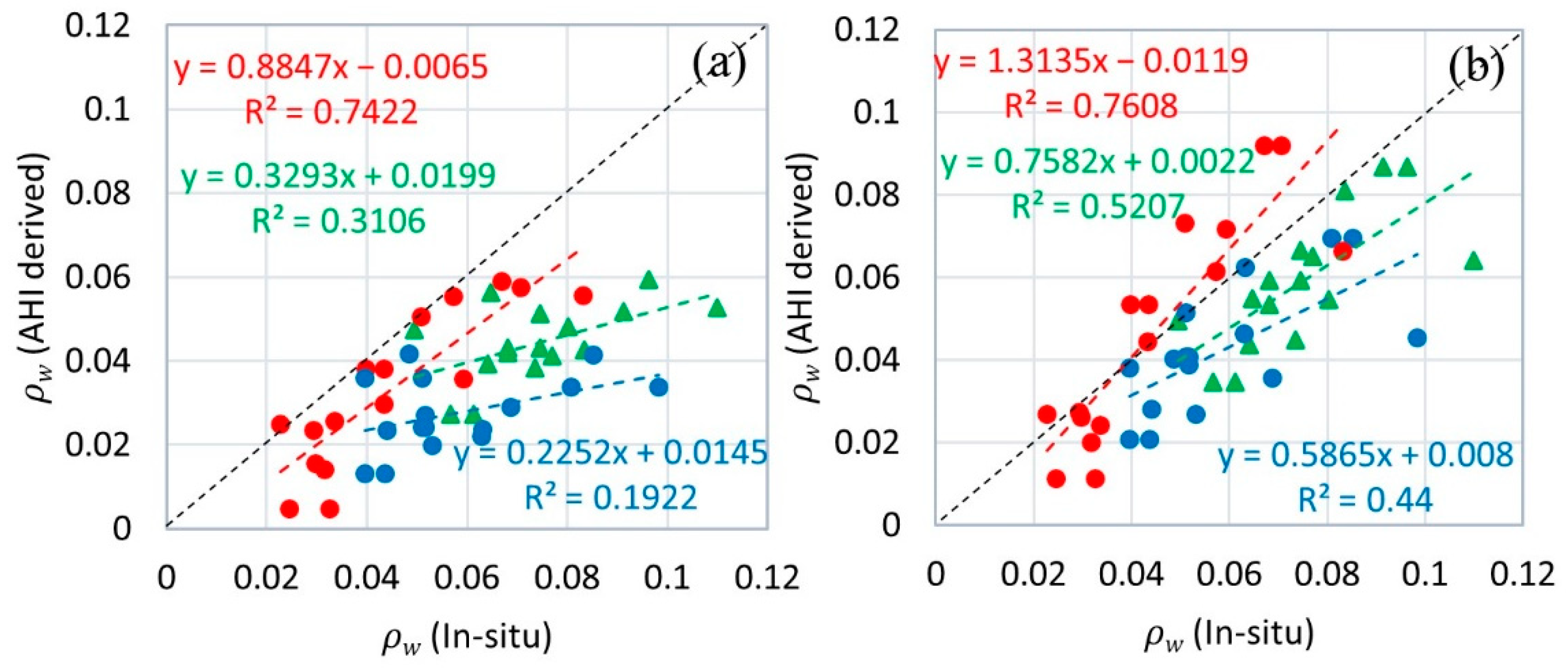
3.2. In-Situ Validation of Water-Leaving Reflectance

Validation of AHI-derived water leaving reflectance (AHI-${\rho }_w$) in visible bands, using both atmospheric approaches, was performed using in-situ TriOS hyperspectral data that were collected within ±5 min of the AHI image acquisition time. The AHI pixel was selected after matching the geographical location of in-situ data with the closest pixel of the AHI image. For accuracy assessment, R, RMSE, and APD were used for AHI-${\rho }_w$ validation. The validation results are shown in

Table 5. In-situ validation of the water-leaving reflectance (${\rho }_w)$ derived from the AHI in visible bands corrected using the NIR-SWIR and SWIR approaches.

	Band 1 (440 nm)		Band 2 (510 nm)		Band 3 (640 nm)
${\mathit{\rho }}_{\mathit{w}}$	NIR-SWIR	SWIR	NIR-SWIR	SWIR	NIR-SWIR	SWIR
R	0.43	0.66	0.55	0.72	0.86	0.87
MAE	0.031	0.016	0.030	0.016	0.012	0.012
RMSE	0.034	0.02	0.032	0.019	0.014	0.014
APD	124%	47%	71%	31%	94%	38%

, for AHI band 1 (blue-470 nm), 2 (green-510 nm), and 3 (red-640 nm). The correlation coefficient, R, for the green and red band, shows a reasonable correlation (>0.5) for both the NIR-SWIR and SWIR methods. However, the SWIR method shows better results than the NIR-SWIR method for the blue band. The NIR-SWIR method underestimated the blue band by 124%. The overall reasonable value of R suggests that these methods could be used to derive AHI-${\rho }_w$ when water reflected reasonably in visible bands. For instance, the highest in-situ values of reflectance in blue, green, and red bands were 0.09, 0.1, and 0.08. Dorji, et al. [58] showed in their study that AHI could not be used reliably at low reflectance values (clear seawater). The R, APD, and MSRE results suggest that the SWIR method outperformed the NIR-SWIR method in all visible bands (Table 5). The lowest RMSE of 0.014 and the highest R of 0.87 was observed for band 3, as compared to the other two visible bands that were corrected using the same approach. Figure 5 shows the scatter plot between in-situ ${\rho }_w$and AHI-${\rho }_w$.

3.3. Calibration and Validation of the Regional TSS Model

A new regional TSS model was developed on the basis of the AHI red and green band. First, the AHI red band threshold value$, R_{rs}\left(640 \mathrm{nm}\right)$ ≥ 0.01 $s{r}^{-1},$was used to classify water in two different water classes, low TSS water class, and moderate-high TSS water class. [59] also used this threshold value for $R_{rs}\left(740 \mathrm{nm}\right)$ to classify water in different water-types, before developing the TSS model. In this study, the threshold was selected based on in-situ hyperspectral data and corresponding TSS concentrations. When TSS concentration was low$, R_{rs}\left(640 \mathrm{nm}\right)$ < 0.01 $s{r}^{-1}$, the green band was more significant to estimate the TSS, and as TSS concentration increased, the red band became more significant for estimating the TSS. Figure 6a shows the correlation between AHI-green band and in-situ TSS and Figure 6b shows correlation between AHI-red band and in-situ TSS. Where, $R_{rs}\left(640 \mathrm{nm}\right)$ < 0.01 $s{r}^{-1}$, AHI’s green-band-based linear model (Equation (24)) was used to estimate TSS, and where$R_{rs}\left(640 \mathrm{nm}\right)$ ≥ 0.01 $s{r}^{-1}$, AHI’s red-band-based linear model (Equation (25)) was used to estimate TSS. About 80% and 20% split was used to develop and validate the regional model, respectively. Figure 6c shows the model validation. Within the validation dataset, the developed model estimated low and high TSS with reasonable accuracy, resulting in an MAE of 0.2 mg/L, RMSE of 0.2 mg/L, and APD of 11% for TSS < 10 mg/L, and MAE of 3.1 mg/L, RMSE of 4.3 mg/L, and APD of 10% for TSS > 10 mg/L. Overall, the models performed well, exhibiting a determination coefficient R² of 0.86 and an overall MAE of 2.2 mg/L, RMSE of 3.6 mg/L, and APD of 11%.

$$TSS=324.38 \times R_{rs}\left(510\right)$$

(24)

$$TSS=2214.8 \times R_{rs}\left(640\right)$$

(25)

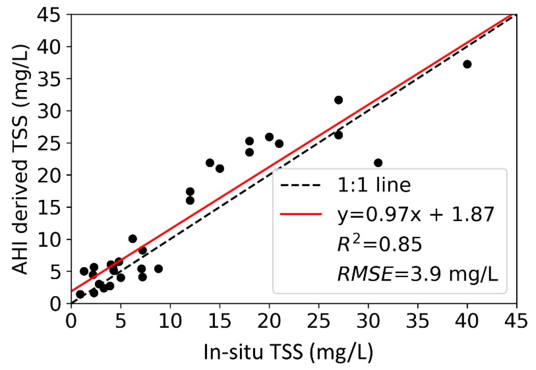
3.4. Validating TSS Model Using AHI Data

Before using the developed TSS model to map hourly TSS concentrations, The TSS model was evaluated using atmospherically corrected AHI data. Section 3.2. shows that the SWIR atmospheric correction approach outperformed the NIR-SWIR approach, when validated with in-situ water leaving reflectance with respect to the AHI bands. Therefore, the cloud-free AHI images from 2016–2019, corrected using the SWIR approach and same–day-station-based TSS data collected by EPD, Hong Kong, was used for validation of the TSS model. The regionally tuned model estimated TSS ≥ 10 mg/L better (R = 0.83, MAE = 4.9 mg/L, RMSE = 4.9 mg/L, and APD = 19% ) than TSS < 10 mg/L (R = 0.53, MAE = 1.8 mg/L, RMSE = 2.1 mg/L, and APD = 38%). Overall determination coefficient R² of 0.85 with MAE of 3.1 mg/L, RMSE of 3.9 mg/L, and APD 30% was observed between the in-situ and AHI-derived TSS measurements (Figure 7).

3.5. Hourly TSS Concentration Mapping

Hourly TSS concentrations were mapped using atmospherically corrected AHI data over the study area on 19 December 2016 from 10:00–15:00 (HKT), at a spatial resolution of 2 km (Figure 8a). From the hourly spatial distribution maps, it was found that the TSS concentrations decreased along the PRE from 10:00–15:00 HKT. The hourly average TSS graph showed that the TSS concentration was around 50 mg/L in the Western Huangmao River estuary in the morning and increased to 57 mg/L in the afternoon at 13:00 HKT and decreased to 53 mg/L in the late afternoon at 15:00 HKT (blue line in Figure 8b). Likewise, TSS concentrations increased along the lower reach of the PRE from 20 mg/L to 26 mg/L from 10:00–15:00 HKT (red line in Figure 8b). However, the diurnal changes in TSS over clear sea water that the model detected were minimum (green line in Figure 8c). The average TSS difference observed over clear seawater was only 0.3 mg/L from 10:00–15:00 HKT. However, the difference was significant in the coastal areas. This might suggest that the changes in water reflectance were due to changes in the TSS concentration rather than changes in solar geometry throughout the day.

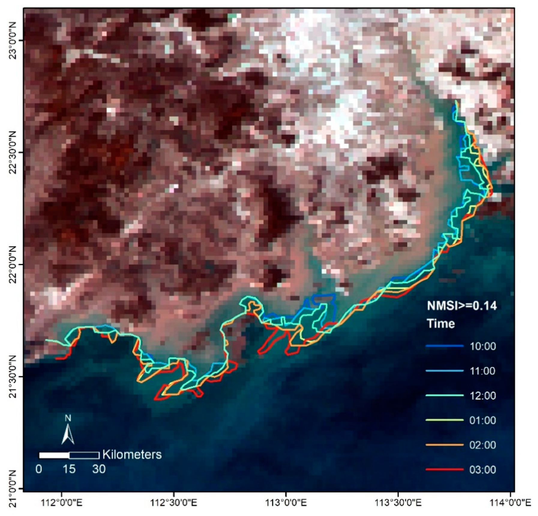
3.6. Validation of Diurnal Variation in Turbidity Front

Diurnal variation in turbidity fronts due to the wind, tides, and upwelling could also be monitored using the NSMI [20]. In this study, the NSMI values were assessed and an NSMI value >= 0.14 was further used as the threshold value for tracking the changes in the turbidity front, as the NSMI value 0.14 corresponded to the TSS value 20 mg/L. The value of NSMI increased as the suspended material increased. Figure S3 of supplementary data shows the variation in NSMI during daytime from 10:00–15:00 HKT, with a half-hourly difference. It was found that the noise in the clear water regions increased in the afternoon. Vanhellemont, et al. [60] also mentioned that the remote-sensing reflectance ($R_{rs}$) became the highest at local noon when considering pure water (TSS Min = 0.0 mg/L). They further concluded that in the geostationary satellites, variation in $R_{rs}$as a result of varying satellite-solar geometry was minimal for highly turbid waters. Therefore, we expect that the changes observed in the turbidity fronts (Figure 9) were the results of the actual changes in turbidity rather than the diurnal variation in water reflectance caused by the changes in solar zenith and azimuth angles, during the daytime. Figure 9 shows the changes in the turbidity front (TSS contour of 20 mg/L) observed from the AHI data during the daytime. This part of the study concluded that AHI data could be used for monitoring diurnal TSS changes, as the clouds have a great impact on the data available from other ocean color satellites; thus, data gaps in ocean color satellites due to cloud cover can also be filled by the AHI images.

4. Discussion

In this study, we investigated the mapping of TSS concentrations with Himawari-8’s AHI sensor in the Pearl River estuary (PRE) and adjacent coastal waters. The study evaluated the possibility and limitations for mapping high temporal variation in TSS concentrations in the study area. AHI can capture multiple images per day. However, changing solar geometry (solar zenith and solar azimuth angle) throughout the day have substantial impacts on the collected satellite radiance ($L_{toa}$). A previous study by Dorji, et al. [58] shows that the $L_{toa}$ in the AHI red band decreased by 31.9% (from 13.2 to 9.0 W m⁻² μm⁻¹ sr⁻¹) from 10:00 to 15:00, in the Australian coastal waters. Thus, it is critical to consider the solar geometry when performing atmospheric correction of AHI. Otherwise, such a large variation would result in a high relative error in the AHI water-leaving reflectance (${\rho }_w$) data and thus in the final resulting TSS product. In the current study, which studied the varying solar geometry, two separate atmospheric correction approaches—the NIR-SWIR approach (using band 4 and 5) and the SWIR approach (using band 5 and 6), were used to derive the ${\rho }_w$differently. For the three test regions,${\rho }_w$in AHI (bands 1 to 3) retrieved by the SWIR atmospheric correction approach outperformed the NIR-SWIR approach. The NIR-SWIR atmospheric correction approach was established on the hypothesis that ${\rho }_w$ in the NIR band was nearly zero; however, visual collection of clear seawater data from box C could have caused the presence of pixels with ${\rho }_w$greater than zero, and thus potentially increased the estimation of the aerosol reflectance ratio ε(4,5). Moreover, the use of a median value of ε for the whole image could also have contributed to the lower accuracy of the NIR-SWIR approach as ε can be changed for each pixel, as ${\rho }_a$ was not necessarily spatially homogenous, especially near the coast, where the water turbidity was more variable. The median value of ε(4,5) was also always higher than the Median values of ε(5,6) for the available data in this study. Neukermans, et al. [22] and Vanhellemont and Ruddick [4] also proved that the combination of shorter and longer wavelengths (NIR-SWIR) resulted in higher values of ε than the combination of longer wavelengths (SWIRs) for SEVIRI and OLI, respectively. Vanhellemont and Ruddick [4] also found that in areas of high turbidity, the SWIR method gave higher and more reliable TSS values than the VIR-NIR approach, as the resulting ${\rho }_w$ was higher using the longer wavelength as compared to that using shorter NIR wavelengths. Our study also showed similar results by estimating higher ${\rho }_w$by the SWIR approach than the NIR-SWIR approach. Due to the lower ${\rho }_w$ estimation by the NIR-SWIR atmospheric correction approach, the derived TSS concentrations were also lower than TSS, which was derived by the SWIR atmospheric corrected data as input. Overall, a lower accuracy was found for the NIR-SWIR approach than for the SWIR approach, when compared to the in-situ spectral data. The correlation coefficients, R, for the red band were the highest for both atmospheric correction approaches.

A wide range of in-situ TSS data (0.6–114 mg/L) was used, along with spectral data to develop a new regional AHI-based TSS model, using the green and red bands of AHI. We validated the algorithm for the study area, and the results showed a good agreement across the TSS range of 1.0–50.8 mg/L. The AHI-based TSS validation using atmospherically corrected AHI data produced an overall R² of 0.85, MAE of 3.1 mf/L, RMSE of 3.9 mg/L, and APD 30%. Atmospherically corrected AHI data also displayed diurnal variation in TSS. It was found that the AHI-based TSS maps could be produced at high frequency with acceptable precisions for TSS ≤ 114 mg/L. Nonetheless, TSS occasionally crossed this upper limit [61]. In the study area, total inorganic particles and turbidity were proportional to TSS [61]. However, organic substances also contributed to TSS [62], and optical properties were also affected by Color Dissolved Organic Matter (CDOM) [63]. Moreover, normally Chl-a concentration has a much smaller variation than TSS, with an average value of 3.11 mg/m⁻³ [62], thus affecting only the blue and green portions of the electromagnetic spectrum. TSS concentrations in the estuarine area were usually moderate-high and the water reflected significantly in the red band. Therefore, the regional TSS algorithm relies on the AHI’s red band. Absorption effects of CDOM largely weakens in red and NIR bands [63] and the best correlation band shift from red to NIR with increasing TSS concentration [64]. Therefore, there is a need to study changes in the spectral combination of red and NIR band due to high TSS concentrations where the red band becomes saturated.

The AHI is featured by a higher temporal resolution (10 min for the whole earth disk) and it covers a spatial area much greater than the only available geostationary ocean color sensor, GOCI. When the ultra-high image capturing frequency is adopted, AHI is capable of divulging the diurnal variation of TSS in turbid estuarine plumes. This study demonstrates that applying a suitable atmospheric correction method to AHI images can provide useful information on the diurnal dynamic of TSS concentrations. Such information would help improve the environmental monitoring and management of coastal waters within the target region of Himawari-8.

Himawari-8 is a meteorological satellite by design and AHI onboard Himawari-8 is not formerly constructed to study water quality parameters. Therefore, the signal-to-noise ratio (SNR) for the visible-Short wave infrared bands of AHI is inferior to that of the specially constructed ocean color sensors. This low SNR might also add discrepancy between the TSS derived from the AHI and the in-situ measured TSS concentrations. However, previous studies by Vanhellemont, et al. [60] showed that the noise equivalent errors in TSS due to SNR in geostationary satellite data could be reduced by temporal averaging 10 min data to the hourly interval, without losing the temporal changes of TSS concentrations due to tidal variations. Furthermore, the current AHI processing, proposed in this study and the TSS algorithm used, still needs to be further investigated with the aid of large in-situ water leaving reflectance data and diurnal in-situ TSS data. However, this study shows that there is a potential for using AHI data to establish operational implementation and near-real-time data analysis for TSS mapping.

5. Conclusions

This study demonstrates the ability of the Himawari-8 AHI sensor in monitoring Total Suspended Solids (TSS) concentrations in moderately turbid to highly turbid coastal waters of the Pearl River Estuary and adjacent coastal areas. The NIR-SWIR and SWIR atmospheric correction approaches were adopted in this paper for the atmospheric correction of AHI data to study the ocean color. AHI-derived remote-sensing reflectance (R_rs), using the SWIR approach, in the red band (640 nm) and the green band (510 nm) shows a high correlation with in-situ R_rs. The R_rs in the red band results in the lowest RMSE, when corrected using the NIR-SWIR and SWIR atmospheric correction methods. The regional AHI-based algorithm was developed for the TSS retrievals. This locally tuned TSS model performed well within the validation dataset, exhibiting a determination coefficient R² of 0.86 and returning RMSE values of 3.6 mg/L. AHI-derived TSS concentrations were also consistent with in-situ TSS concentrations, producing R² = 0.85, MAE = 3.1 mg/L, RSME = 3.9 mg/L, and APD = 30%. AHI can provide more data for mapping diurnal TSS variations. Thus, atmospherically corrected AHI data based on the SWIR method can be used to capture the diurnal pattern of TSS concentrations and changes in turbidity at ultrahigh temporal resolution (every 10 min). TSS concentrations up to 114 mg/L can be mapped with high accuracy. Moreover, this can be done for fairly low TSS concentrations from ∼1.0 mg/L upwards (TSS∼114 mg/L). In summer afternoons, only TSS concentrations before 1:00 pm HKT could be derived over the study area, due to high sun-glint afterwards. These TSS measurements at high frequency provide not only detailed information for efficient environmental monitoring but are also important for gap filling in ocean color satellite data, and help researchers to better understand the TSS dynamics in sensitive coastal and estuarine environments.

References

1. Bernardo, N.; Watanabe, F.; Rodrigues, T.; Alcântara, E. Evaluation of the suitability of MODIS, OLCI and OLI for mapping the distribution of total suspended matter in the Barra Bonita Reservoir (Tietê River, Brazil). Remote Sens. Appl. Soc. Environ. 2016, 4, 68–82. [Google Scholar] [CrossRef]
2. Binding, C.E.; Bowers, D.G.; Mitchelson, J.E.G. An algorithm for the retrieval of suspended sediment concentrations in the Irish Sea from SeaWiFS ocean colour satellite imagery. Int. J. Remote Sens. 2003, 24, 3791–3806. [Google Scholar] [CrossRef]
3. Blix, K.; Pálffy, K.; Tóth, V.R.; Eltoft, T. Remote sensing of water quality parameters over Lake Balaton by using Sentinel-3 OLCI. Water 2018, 10, 1428. [Google Scholar] [CrossRef] [Green Version]
4. Vanhellemont, Q.; Ruddick, K. Advantages of high quality SWIR bands for ocean colour processing: Examples from Landsat-8. Remote Sens. Environ. 2015, 161, 89–106. [Google Scholar] [CrossRef] [Green Version]
5. Viollier, M.; Sturm, B. CZCS data analysis in turbid coastal water. J. Geophys. Res. Atmos. 1984, 89, 4977–4985. [Google Scholar] [CrossRef]
6. Fettweis, M.; Nechad, B.; Eynde, D. An estimate of the suspended particulate matter (SPM) transport in the southern North Sea using SeaWiFS images, in situ measurements and numerical model results. Cont. Shelf Res. 2007, 27, 1568–1583. [Google Scholar] [CrossRef] [Green Version]
7. Chen, X.; Han, X.; Feng, L. Towards a practical remote-sensing model of suspended sediment concentrations in turbid waters using MERIS measurements. Int. J. Remote Sens. 2015, 36, 3875–3889. [Google Scholar] [CrossRef]
8. Doxaran, D.; Lamquin, N.; Park, Y.; Mazeran, C.; Ryu, J.H.; Wang, M.; Poteau, A. Retrieval of the seawater reflectance for suspended solids monitoring in the East China Sea using MODIS, MERIS and GOCI satellite data. Remote Sens. Environ. 2014, 146, 36–48. [Google Scholar] [CrossRef]
9. Kratzer, S.; Brockmann, C.; Moore, G. Using MERIS full resolution data to monitor coastal waters—A case study from Himmerfjärden, a fjord-like bay in the northwestern Baltic Sea. Remote Sens. Environ. 2008, 112, 2284–2300. [Google Scholar] [CrossRef]
10. Chen, S.; Huang, W.; Wang, H.; Li, D. Remote sensing assessment of sediment re-suspension during Hurricane Frances in Apalachicola Bay, USA. Remote Sens. Environ. 2009, 113, 2670–2681. [Google Scholar] [CrossRef]
11. Chen, S.; Han, L.; Chen, X.; Li, D.; Sun, L.; Li, Y. Estimating wide range Total Suspended Solids concentrations from MODIS 250-m imageries: An improved method. ISPRS J. Photogramm. Remote Sens. 2015, 99, 58–69. [Google Scholar] [CrossRef]
12. Miller, R.L.; McKee, B.A. Using MODIS Terra 250 m imagery to map concentrations of total suspended matter in coastal waters. Remote Sens. Environ. 2004, 93, 259–266. [Google Scholar] [CrossRef]
13. National Snow and Ice Data Center. MODIS to VIIRS: Building a Time Series. National Snow and Ice Data Center. Available online: https://nsidc.org/nsidc-monthly-highlights/2017/08/modis-viirs-building-time-series (accessed on 13 January 2021).
14. Toming, K.; Kutser, T.; Uiboupin, R.; Arikas, A.; Vahter, K.; Paavel, B.J.R.S. Mapping water quality parameters with sentinel-3 ocean and land colour instrument imagery in the Baltic Sea. Remote Sens. 2017, 9, 1070. [Google Scholar] [CrossRef] [Green Version]
15. Li, J.; Gao, S.; Wang, Y. Delineating suspended sediment concentration patterns in surface waters of the Changjiang Estuary by remote sensing analysis. Acta Oceanol. Sin. 2010, 29, 38–47. [Google Scholar] [CrossRef]
16. Munday, J.C., Jr.; Alföldi, T.T. Landsat test of diffuse reflectance models for aquatic suspended solids measurement. Remote Sens. Environ. 1979, 8, 169–183. [Google Scholar] [CrossRef]
17. Onderka, M.; Pekárová, P. Retrieval of suspended particulate matter concentrations in the Danube River from Landsat ETM data. Sci. Total Environ. 2008, 397, 238–243. [Google Scholar] [CrossRef] [PubMed]
18. Wang, J.J.; Lu, X.X.; Liew, S.C.; Zhou, Y. Retrieval of suspended sediment concentrations in large turbid rivers using Landsat ETM+: An example from the Yangtze River, China. Earth Surf. Process. Landf. 2009, 34, 1082–1092. [Google Scholar] [CrossRef]
19. Hafeez, S.; Wong, M.S. Measurement of Coastal Water Quality Indicators Using Sentinel-2; An Evaluation Over Hong Kong and the Pearl River Estuary. In Proceedings of the IGARSS 2019—2019 IEEE International Geoscience and Remote Sensing Symposium, Yokohama, Japan, 28 July–2 August 2019; pp. 8249–8252. [Google Scholar]
20. Munirm, M.; Ramadhan, A.F.; Nastiti, A.; Putri, A.A.; Bawono, M.R.K.S.; Nur, Z. Utilization of Sentinel-2A imagery For Mapping The dynamics of Total Suspended Sediment at The River Mouth of The Padang City. In Proceedings of the 2019 5th International Conference on Science and Technology (ICST), Yogyakarta, Indonesia, 30–31 July 2019; Volume 1, pp. 1–6. [Google Scholar]
21. Saberioon, M.; Brom, J.; Nedbal, V.; Souček, P.; Císař, P. Chlorophyll-a and total suspended solids retrieval and mapping using Sentinel-2A and machine learning for inland waters. Ecol. Indic. 2020, 113, 106236. [Google Scholar] [CrossRef]
22. Neukermans, G.; Ruddick, K.; Bernard, E.; Ramon, D.; Nechad, B.; Deschamps, P.Y. Mapping total suspended matter from geostationary satellites: A feasibility study with SEVIRI in the Southern North Sea. Opt. Express 2009, 17, 14029–14052. [Google Scholar] [CrossRef] [PubMed] [Green Version]
23. Thompson, C.E.L.; Couceiro, F.; Fones, G.R.; Helsby, R.; Amos, C.L.; Black, K.; Parker, E.R.; Greenwood, N.; Statham, P.J.; Kelly-Gerreyn, B.A. In situ flume measurements of resuspension in the North Sea. Estuar. Coast. Shelf Sci. 2011, 94, 77–88. [Google Scholar] [CrossRef] [Green Version]
24. Neukermans, G.; Ruddick, K.; Greenwood, N. Diurnal variability of turbidity and light attenuation in the southern North Sea from the SEVIRI geostationary sensor. Remote Sens. Environ. 2012, 124, 564–580. [Google Scholar] [CrossRef]
25. Ruddick, K.; Vanhellemont, Q.; Yan, J.; Neukermans, G.; Wei, G.; Shang, S. Variability of suspended particulate matter in the Bohai Sea from the geostationary Ocean Color Imager (GOCI). Ocean Sci. J. 2012, 47, 331–345. [Google Scholar] [CrossRef]
26. Hu, Z.; Pan, D.; He, X.; Bai, Y. Diurnal variability of turbidity fronts observed by geostationary satellite ocean color remote sensing. Remote Sens. 2016, 8, 147. [Google Scholar] [CrossRef] [Green Version]
27. Mao, Y.; Wang, S.; Qiu, Z.; Sun, D.; Bilal, M. Variations of transparency derived from GOCI in the Bohai Sea and the Yellow Sea. Opt. Express 2018, 26, 12191–12209. [Google Scholar] [CrossRef]
28. Lou, X.; Hu, C. Diurnal changes of a harmful algal bloom in the East China Sea: Observations from GOCI. Remote Sens. Environ. 2014, 140, 562–572. [Google Scholar] [CrossRef]
29. Qi, L.; Hu, C.; Visser, P.M.; Ma, R. Diurnal changes of cyanobacteria blooms in Taihu Lake as derived from GOCI observations. Limnol. Oceanogr. 2018, 63, 1711–1726. [Google Scholar] [CrossRef] [Green Version]
30. Murakami, H. Ocean color estimation by Himawari-8/AHI. In Remote Sensing of the Oceans and Inland Waters: Techniques, Applications, and Challenges; International Society for Optics and Photonics: Bellingham, WA, USA, 2016; Volume 9878, p. 987810. [Google Scholar]
31. Chen, X.; Shang, S.; Lee, Z.; Qi, L.; Yan, J.; Li, Y. High-frequency observation of floating algae from AHI on Himawari-8. Remote Sens. Environ. 2019, 227, 151–161. [Google Scholar] [CrossRef]
32. Ryu, J.H. GOCI Statusand GOCI-II Plan. Available online: https://iocs.ioccg.org/wp-content/uploads/0915-joo-hyung-ryu-agency-report.pdf (accessed on 13 January 2021).
33. Zhou, Q.; Tian, L.; Wai, O.W.; Li, J.; Sun, Z.; Li, W. High-Frequency Monitoring of Suspended Sediment Variations for Water Quality Evaluation at Deep Bay, Pearl River Estuary, China: Influence Factors and Implications for Sampling Strategy. Water 2018, 10, 323. [Google Scholar] [CrossRef] [Green Version]
34. Tang, C.; Zhou, D.; Endler, R.; Lin, J.; Harff, J. Sedimentary development of the Pearl River Estuary based on seismic stratigraphy. J. Mar. Syst. 2010, 82, S3–S16. [Google Scholar] [CrossRef]
35. Justesen, P.; Ellegaard, A.C.; Bernitt, L.; Lu, Q. 2-D & 3-D modeling of Hong Kong waters. In Proceedings of the Second International Conference of Hydrodynamics; Balkema: Rotterdam, The Netherlands, 1996; pp. 649–654. [Google Scholar]
36. Jayawardena, A.W.; Lai, F. Time series analysis of water quality data in Pearl River, China. J. Environ. Eng. 1989, 115, 590–607. [Google Scholar] [CrossRef]
37. Zhan, W.; Wu, J.; Wei, X.; Tang, S.; Zhan, H. Spatio-temporal variation of the suspended sediment concentration in the Pearl River Estuary observed by MODIS during 2003–2015. Cont. Shelf Res. 2019, 172, 22–32. [Google Scholar] [CrossRef]
38. Chen, C.; Tang, S.; Pan, Z.; Zhan, H.; Larson, M.; Jönsson, L. Remotely sensed assessment of water quality levels in the Pearl River Estuary, China. Mar. Pollut. Bull. 2007, 54, 1267–1272. [Google Scholar] [CrossRef] [PubMed]
39. Yin, K. Influence of monsoons and oceanographic processes on red tides in Hong Kong waters. Mar. Ecol. Prog. Ser. 2003, 262, 27–41. [Google Scholar] [CrossRef] [Green Version]
40. Yukio, K.H.M.; Misako, K. Himawari-8 SST by JAXA, Japan Aerospace Exploration Agency (JAXA); Earth Observation Research Center (EORC): Melbourne, Australia, 2015; Available online: http://adf5c324e923ecfe4e0a-6a79b2e2bae065313f2de67bbbf078a3.r67.cf1.rackcdn.com/Melbourne%20Workshop%202015%20-%20Monday%209th%20November%202015/M08satelliteoceanographywsmelbourneyukiokurihara.pdf (accessed on 13 January 2021).
41. Japan Meteorological Agency. Himawari-8/9Himawari Standard DataUser’s Guide. Available online: https://www.data.jma.go.jp/mscweb/en/himawari89/space_segment/hsd_sample/HS_D_users_guide_en_v12.pdf (accessed on 13 January 2021).
42. Monitor, J.H. JAXA Himawari Monitor. Available online: https://www.eorc.jaxa.jp/ptree/userguide.html (accessed on 13 January 2021).
43. Ruddick, K.G.; Ovidio, F.; Rijkeboer, M. Atmospheric correction of SeaWiFS imagery for turbid coastal and inland waters. Appl. Opt. 2000, 39, 897–912. [Google Scholar] [CrossRef] [PubMed] [Green Version]
44. Gordon, H.R.; Wang, M. Influence of oceanic whitecaps on atmospheric correction of ocean-color sensors. Appl. Opt. 1994, 33, 7754–7763. [Google Scholar] [CrossRef] [PubMed]
45. Vermote, E.F.; Tanré, D.; Deuze, J.L.; Herman, M.; Morcette, J.J. Second simulation of the satellite signal in the solar spectrum, 6S: An overview. IEEE Trans. Geosci. Remote Sens. 1997, 35, 675–686. [Google Scholar] [CrossRef] [Green Version]
46. Proud, S.R.; Fensholt, R.; Rasmussen, M.O.; Sandholt, I. A comparison of the effectiveness of 6S and SMAC in correcting for atmospheric interference of Meteosat Second Generation images. J. Geophys. Res. Atmos. 2010, 115, D17. [Google Scholar] [CrossRef]
47. NASA. Giovanni the Bridge Between Data and Science v 4.34. Available online: https://giovanni.gsfc.nasa.gov/giovanni (accessed on 13 January 2021).
48. Wang, M.; Shi, W. Cloud masking for ocean color data processing in the coastal regions. IEEE Trans. Geosci. Remote Sens. 2006, 44, 3196–3205. [Google Scholar] [CrossRef]
49. Vanhellemont, Q.; Ruddick, K. Atmospheric correction of metre-scale optical satellite data for inland and coastal water applications. Remote Sens. Environ. 2018, 216, 586–597. [Google Scholar] [CrossRef]
50. Gordon, H.R.; Wang, M. Retrieval of water-leaving radiance and aerosol optical thickness over the oceans with SeaWiFS: A preliminary algorithm. Appl. Opt. 1994, 33, 443–452. [Google Scholar] [CrossRef]
51. Mueller, J.L.; Morel, A.; Frouin, R.; Davis, C.; Arnone, R.; Carder, K.; Lee, Z.P.; Sterward, R.G.; Hooker, S.; Mobley, C.D.; et al. Ocean Optics Protocols for Satellite Ocean Color Sensor Validation, Revision 4. Volume III: Radiometric Measurements and Data Analysis Protocols; Goddard Space Flight Space Center: Greenbelt, MD, USA, 2003; Volume 3.
52. Ruddick, K.; Cauwer, V.; Mol, B. Use of the near infrared similarity reflectance spectrum for the quality control of remote sensing data. In Remote Sensing of the Coastal Oceanic Environment; International Society for Optics and Photonics: Bellingham, WA, USA, 2005; Volume 5885, p. 588501. [Google Scholar]
53. Mobley, C.D. Estimation of the remote-sensing reflectance from above-surface measurements. Appl. Opt. 1999, 38, 7442–7455. [Google Scholar] [CrossRef] [PubMed]
54. Strickland, J.D.H.; Parsons, T.R. A Practical Handbook of Seawater Analysis, 2nd ed.; Fisheries Research Board of Canada: Ottawa, ON, Canada, 1972. [Google Scholar]
55. EPD. Marine Water Quality Data. Available online: http://epic.epd.gov.hk/EPICRIVER/marine/?lang=en (accessed on 13 January 2021).
56. Hafeez, S.; Wong, M.S.; Ho, C.H.; Nazeer, M.; Nichol, J.; Abbas, S.; Tang, D.; Lee, K.H.; Pun, L. Comparison of machine learning algorithms for retrieval of water quality indicators in case-II waters: A case study of Hong Kong. Remote Sens. 2019, 11, 617. [Google Scholar] [CrossRef] [Green Version]
57. Montalvo, L.G. Spectral Analysis of Suspended Material in Coastal Waters: A Comparison Between Band Math Equations. 2010. Available online: https://docplayer.net/39330139-Spectral-analysis-of-suspended-material-in-coastal-waters-a-comparison-between-band-math-equations.html (accessed on 13 January 2021).
58. Dorji, P.; Fearns, P. Atmospheric correction of geostationary Himawari-8 satellite data for Total Suspended Sediment mapping: A case study in the Coastal Waters of Western Australia. ISPRS J. Photogramm. Remote Sens. 2018, 144, 81–93. [Google Scholar] [CrossRef]
59. Balasubramanian, S.V.; Pahlevan, N.; Smith, B.; Binding, C.; Schalles, J.; Loise, H.; Gurlin, D.; Greb, S.; Alikas, K.; Randla, M.; et al. Robust algorithm for estimating total suspended solids (TSS) in inland and nearshore coastal waters. Remote Sens. Environ. 2020, 246, 111768. [Google Scholar] [CrossRef]
60. Vanhellemont, Q.; Neukermans, G.; Ruddick, K. Synergy between polar-orbiting and geostationary sensors: Remote sensing of the ocean at high spatial and high temporal resolution. Remote Sens. Environ. 2014, 146, 49–62. [Google Scholar] [CrossRef] [Green Version]
61. Xing, Q.; Lou, M.; Chen, C.; Shi, P. Using in situ and satellite hyperspectral data to estimate the surface suspended sediments concentrations in the Pearl River estuary. IEEE J. Sel. Top. Appl. Earth Obs. Remote Sens. 2013, 6, 731–738. [Google Scholar] [CrossRef]
62. Liu, D.; Fu, D.; Xu, B.; Shen, C. Estimation of total suspended matter in the Zhujiang (Pearl) River estuary from Hyperion imagery. Chin. J. Oceanol. Limnol. 2012, 30, 16–21. [Google Scholar] [CrossRef]
63. Zhang, Y.; Lin, H.; Chen, C.; Chen, L.; Zhang, B.; Gitelson, A.A. Estimation of chlorophyll-a concentration in estuarine waters: Case study of the Pearl River estuary, South China Sea. Environ. Res. Lett. 2011, 6, 24016. [Google Scholar] [CrossRef]
64. Tang, S.; Dong, Q.; Chen, C.; Liu, F.; Jin, G. Retrieval of suspended sediment concentration in the pearl river estuary from meris using support vector machines. In Proceedings of the 2009 IEEE International Geoscience and Remote Sensing Symposium, Cape Town, South Africa, 12–17 July 2009; Volume 3, pp. 239–242. [Google Scholar]
Figure 1. (a) Advanced Himawari Imager (AHI) true-color image of the study area captured on 2 February 2016 at 10:00 (HKT). All bands were aggregated to a 2-km spatial resolution. Box A corresponds to very turbid coastal water (river plume), box B corresponds to moderately turbid water, and box C corresponds to the homogenous clearwater area, (b) in-situ hyperspectral data collected during field campaigns in August 2014, January 2018, and January 2019, (c) in-situ hyperspectral data collected during field campaigns in May 2018.
Remotesensing 13 00336 g001
Figure 2. Distribution of aerosol reflectance ratio ( ε ), over clear sea water pixels, obtained from the Rayleigh corrected AHI image on 7 February 2016 at 10:00 (HKT); (a) ε ( 5 , 6 ) and (b) ε ( 4 , 5 ) .
Remotesensing 13 00336 g002
Figure 3. (a) In-situ ASD measured R r s   collected during August 2014 campaign in the Pearl River Estuary (PRE), and (b) in-situ TriOS measured R r s collected during January 2018, May 2018 and January 2019 campaigns. The range of total suspended solid (TSS) is 18.5–114 mg/L in (a) and 0.6–70 mg/L in (b).
Remotesensing 13 00336 g003
Figure 4. Scatter plots showing the comparison between NIR-SWIR ρ w and SWIR ρ w at the first four bands of AHI considering highly turbid coastal area (box A) and moderately turbid and algal bloom affected area (box B). (a) AHI band 1 (470 nm), (b) AHI band 2 (510 nm), (c) AHI band 3 (640 nm), and (d) AHI band 4 (856 nm). The colors in the scatterplots denote the pixel counts.
Remotesensing 13 00336 g004
Figure 5. In-situ water leaving reflectance ( ρ w ) and AHI-derived water leaving reflectance match-up pairs for (a) the NIR-SWIR and (b) the SWIR atmospheric correction approach. The colored dotted lines are the best fit lines and black dotted line is 1:1 line.
Remotesensing 13 00336 g005
Figure 6. (a) Calibration of the TSS model based on the AHI green band (Rrs 510 nm). (b) Calibration of the TSS model based on the AHI red band (Rrs 640 nm). (c) TSS match-up analysis with the validation dataset. In the scatterplots (a,b), the superimposed equations are the linear “best-fitting” functions.
Remotesensing 13 00336 g006
Figure 7. Validation of the developed TSS model using the AHI corrected data and same-day in-situ TSS data.
Remotesensing 13 00336 g007
Figure 8. (a) Hourly TSS concentration map based on AHI data on 19 December 2016, (b) average hourly changes in TSS in coastal waters, red line (red box-lower Pearl River estuary), the blue line (blue box-Huangmao River estuary), and (c) the average hourly changes in TSS in seawater green line (black box-clear water).
Remotesensing 13 00336 g008
Figure 9. Diurnal changes in the turbidity front captured by AHI data on 7 February 2016.
Remotesensing 13 00336 g009