A Dual-Channel Aerosol Optical Depth Retrieval Algorithm Incorporating the BRDF Effect from AVHRR over Eastern Asia

Abstract

A NOAA/AVHRR dual-channel method over land is proposed to simultaneously retrieve aerosol optical depth (AOD) at 0.55 μm, and surface reflectance at 0.63 and 0.85 μm. Compared with previous well-established one-channel retrieval algorithms, this algorithm takes advantage of the surface reflectance ratio between 0.63 and 0.85 μm in an attempt to account for the effect induced by the surface bidirectional reflectance distribution function (BRDF). This effect cannot be negligible due to the orbit drift and phasing running of NOAA satellites, both of which potentially cause large solar angular variation. Meanwhile, the observation posture change of AVHRR would cause large sensor angular variation in time series measurements. The used surface reflectance ratio based on dual channels at 0.63 and 0.85 μm is found more reasonable to be assumed as unchanged during a certain period of time, compared to the traditional ratio when addressing the BRDF issue. AOD retrievals have been carried out over Eastern Asia. Validation against aerosol robotic network (AERONET) measurements shows that up to 83% of AOD validation collocations are within error lines (±0.15 ± 0.15τ, $\tau$ is AOD) with an $R$ of 0.88 and an root mean square error (RMSE) of 0.15. The dual-channel algorithm taking into account the surface BRDF effect is proved outperforming the conventional 0.63 μm-channel method. It indicates that our algorithm has the potential to be applied to the retrieval of long series of AOD, especially to the AOD retrieval of the sensors which lack a shortwave infrared channel required in the MODerate resolution Imaging Spectroradiometer (MODIS) dark target AOD algorithm.

1. Introduction

Aerosols play an important role in the regional and global climate through direct interactions with radiation [1,2,3,4] and indirect interactions with clouds [5,6,7,8,9,10,11]. It has been well recognized that satellite retrieved aerosol optical depth (AOD) data is one of the useful data sources to constrain the uncertainties of climate effect induced by intensive anthropogenic activities (e.g., [12]). In particular, the long-term accurate AOD measurement, from either ground-based or satellite-based instruments, can well reflect the trend of local and global air pollution [7,13,14].

Ground-based AOD observations from the aerosol robotic network (AERONET) can provide AOD measurements with high accuracy [15]. However, AERONET is not available before 1997 in eastern Asia. Moreover, it only reflects local aerosol properties near the ground-based stations. In comparison, the Advanced Very High-Resolution Radiometer (AVHRR) series, with global observations observed on a daily basis for 40 years, has become a topic of interest [16,17,18,19,20,21,22].

Numerous previous studies have been dedicated to AVHRR AOD retrieval, especially over oceans, due to water’s low reflectance [23] and its maximum sensitivity to aerosol retrieval [24]. Global AOD distribution over oceans have been retrieved from single-channel [25] and dual-channel algorithms [16,17,26]. The early AVHRR AOD algorithms used channel 1 reflectance measurements by assuming a known aerosol particle size distribution and refractive index, which lead to the underestimation of the AOD values due to the strong temporal and spatial variability of aerosol properties [27,28,29]. Therefore, it is suggested to retrieve AOD and size distribution or refractive index values using multichannel reflectance measurements [26]. One of the attempts was based on the relationship between top-of-atmospheric (TOA) reflectance at 0.63 and 0.85 μm for different aerosol optical properties [17].

The AOD retrieval over land would be more difficult because of the complex heterogeneity of land surface. AVHRR was not primarily designed for aerosol retrieval and fewer channels were available, which would intensify the difficulties of AOD retrieval over land [20,22]. Nevertheless, several studies have investigated the potential of retrieving aerosols over land [18,19,20,21,22]. The accurate surface reflectance estimation is essential to the AOD retrieval. In order to acquire the surface reflectance from the limited AVHRR spectral information, time series images input [30,31] or empirical relationships of surface reflectance between spectral bands [21] are used as a solution. The first method originates from early studies, which found a clear day, namely a day with only the background aerosol, and assumed that the surface reflectance between the clear day and a hazy day did not change. Then, the difference between these two days was used to retrieve the aerosol properties [30,31]. Subsequent studies improved the surface reflectance estimation by finding the clear days from time series images [19,20]. The improved method assumes that the surface reflectance remains unchanged during the 45-day period and that there are several clear days. Because AVHRR scans the earth with large variability of observation postures, the method used the convex hull algorithm to account for the view geometry variation effect on the surface reflectance estimation [19,20]. Its application to Europe showed good results compared with MODerate resolution Imaging Spectroradiometer (MODIS) and Medium Resolution Imaging Spectrometer (MERIS) products [20]. Nevertheless, the method improved by Riffler et al. [20] was applied to a surface reflectance of less than 0.07, restricting its application outside of Europe. Another way of estimating surface reflectance employs the empirical relationship of surface reflectance between the only visible band at 0.63 μm and the 3.75 μm band which is less unaffected by the aerosols [21]. Recently, Hsu et al. [22] developed the AVHRR AOD retrieval algorithm on the basis of the Deep Blue algorithm which has been previously applied to the MODIS, Sea-viewing Wide Field-of-view Sensor (SeaWiFS) and Visible Infrared Imaging Radiometer Suite (VIIRS). The Deep Blue algorithm over land uses a minimum reflectance technique in essence to find the clear day for the pre-established surface reflectance database (according to different scattering angles and normalized difference vegetation index (NDVI) domains) in dry regions. In vegetated regions, the Deep Blue algorithm uses a maximum NDVI to find the clear day and obtains the surface reflectance at 0.63 μm from the Rayleigh-corrected TOA reflectance at 0.85 μm and NDVI (NDVI empirically corrected according to AOD, scattering angle and air mass).

In the process of finding out the clear day from time series measurements, the surface bidirectional reflectance distribution function (BRDF) effect cannot be ignored because of both the solar zenith angle and the view geometry changing considerably during these days. Previous studies have revealed that the National Oceanic and Atmospheric Administration (NOAA) satellites which carry AVHRR sensors underwent orbit drift. The phenomenon means that the transit time varies greatly during the lifetime of satellites, causing a large change in the solar zenith angle [32,33,34]. The solar angular variation can be even larger for the afternoon satellites. Moreover, the phasing running of the NOAA satellites can result in the imaging time of the same pixel on adjacent days reaching ±51 min, leading to the solar angular variation unignorable [35,36]. Besides, the large AVHRR observing posture variation causes the large variation in view geometry. All the above factors lead to an unignorable BRDF effect. Only a few studies have accounted for the BRDF effect [19,20,22]. Further, the surface reflectance at 0.63 μm alone is used to retrieve AOD. However, our forward sensitivity study reveals that in some cases only using the 0.63 μm channel to retrieve AOD may be inadequate and cause large error. Therefore, a dual-channel retrieval algorithm is required. Thus, we go further to take advantage of the surface reflectance ratio between 0.63 and 0.85 μm to estimate the clear day (the least TOA reflectance ratio) and to retrieve AOD instead of the surface reflectance at 0.63 μm. This paper is organized in the following manner. Section 2 introduces the data sets and the preprocess method. The whole algorithm is depicted in detail in Section 3. The need of a dual-channel retrieval algorithm is described firstly. The reason for choosing the surface reflectance ratio to address the BRDF effect is then demonstrated from the theoretical point of view, including the uncertainty study as well. The validation results are presented in Section 4. Finally, the key conclusions are summarized in Section 5.

2. Datasets and Their Preprocessing

We mainly used AVHRR observations as the data source. Besides, AERONET measurements were used to analyze the dual-channel retrieval algorithm and validate the AOD retrieval result. The two datasets are described below.

2.1. AVHRR

The Local Area Coverage (LAC) data of AVHRR/3 was used in this study. AVHRR/3 observes the Earth in the following six spectral bands: 0.58–0.68 μm (channel 1), 0.725–1.0 μm (channel 2), 1.58–1.64 μm (channel 3A), 3.55–3.93 μm (channel 3B), 10.3–11.3 μm (channel 4), and 11.5–12.5 μm (channel 5). The nominal resolution of the LAC data at the nadir is 1.1 km. NOAA uses two satellites, namely a morning satellite and an afternoon satellite, to ensure that the sunlight side of the Earth is observed at least twice every day. In this study, Eastern Asia was selected as the study area (Figure 1). The geographic range covers from 18° N to 54° N and 110° E to 136° E. AVHRR data from July 2008 to June 2010 were collected. During this period, three satellites were involved. NOAA-18 (NN) and NOAA-19 (NP) are the afternoon satellites, while NOAA-17 (NM) is the morning satellite.

The AVHRR data preprocess and gas absorption correction method is described as follows. Firstly, the AVHRR TOA radiance was calibrated into reflectance using the post-launched calibration coefficients from NOAA/National Environmental Satellite Information Data and Information Service (NOAA/NESDIS) [37,38]. Secondly, the clouds were masked using the Clouds from AVHRR Extended System (CLAVR-x) results [39]. We also filtered the oceanic pixels using MODIS land water mask product (MOD44W). Followingly, because snow- or ice-covered surfaces reflect too much light, snow and ice pixels were eliminated, especially in the winter and spring seasons of Eastern Asia. The snow and ice product from global map datasets at 4 × 4 km spatial resolution (ftp://www.orbit.nesdis.noaa.gov/pub/smcd/emb/snow/global_mult_snow_ice/) were used [40]. Then, pixels of which satellite zenith angles larger than 60° or solar zenith angles larger than 63° were discarded because plane parallel approximation was used in the study.

The AVHRR TOA reflectance at 0.63 and 0.85 μm should be corrected to remove the effects of water vapor and ozone because 0.85 μm channel is heavily influenced by a strong water vapor absorption band. The MODIS gas correction method was employed (http://modis.gsfc.nasa.gov/data/atbd/atmos_atbd.php). Products from the Ozone Monitoring Instrument (OMI) on board the NASA Aura satellite were used as ozone input. We recalculated the water vapor absorption coefficients which were adjusted for AVHRR spectral responses using the Second Simulation of a Satellite Signal in the Solar Spectrum-Vector (6SV) radiative transfer code [41]. The formula adopted for water vapor transmission is

$$T_g\left(H_{2}O,M\right)=\exp \left(-\exp \left(a+b\ln \left(M{U}_{H_{2}O}\right)+c{\ln }^2\left(M{U}_{H_{2}O}\right)\right)\right),$$

(1)

where $M$ is the air mass, $U_{H_{2}O}$ is the total precipitable water vapor and we used MOD/MYD07 products as input. Coefficients $a$, $b$, and $c$ were calculated, and the values of $a$, $b$, and $c$ are listed in

Table 1. Water vapor absorption coefficients of AVHRR and MODIS.

Wavelength (μm)	a		b		c
	AVHRR	MODIS	AVHRR	MODIS	AVHRR	MODIS
0.63	−5.5424	−5.7389	0.9083	0.9255	−0.0419	−0.0188
0.85	−2.4187	−5.3296	0.4995	0.8246	−0.0248	−0.0277

. The values of $a$, $b$, and $c$ in 0.63 μm change little from those in MODIS 0.66 μm band, while $a$, $b$, and $c$ values in 0.85 μm are significantly different from those in MODIS 0.86 μm band. It is revealed that different sensor spectral responses (Figure 2) over the water vapor absorption band can cause different water vapor influences. Therefore, the water vapor correction of AVHRR 0.85 μm channel is necessary. In the absence of MOD/MYD07 water vapor data, the global average optical depth values were used and the Beer–Bouguer–Lambert law was adopted (http://modis.gsfc.nasa.gov/data/atbd/atmos_atbd.php).

After the gas absorption correction, the remaining AVHRR pixels were further processed to remove undetected clouds or cloud shadow pixels and resized to a resolution of 11 km, because cloud shadow may contaminate the surface reflectance and mistaking clouds for aerosol could lead to abnormal high AOD retrievals. The brightest 50% and darkest 20% of AVHRR pixels were removed when the TOA reflectance values of channel 1 were between 0 and 0.25, which is similar as what is done in the MODIS pixel pre-selection method.

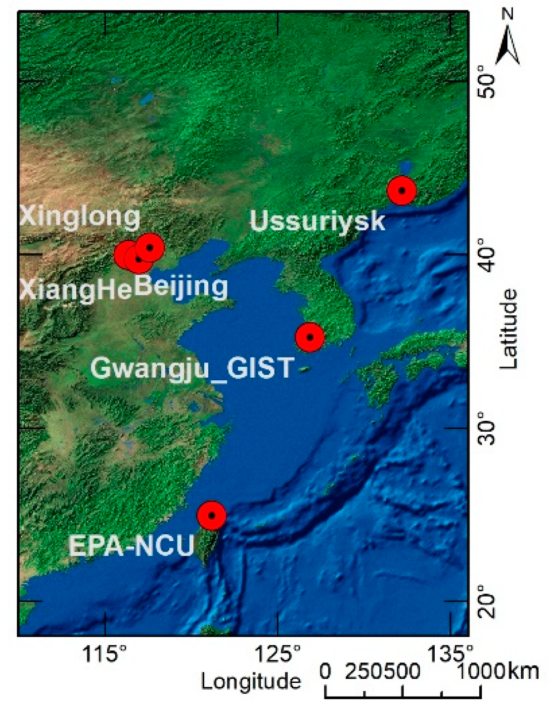
2.2. AERONET Measurements

AERONET is a global network that provides long-term and continuous AOD data with relatively high accuracy and precision [15,42] for validating satellite-based AOD retrievals [43,44]. Overall, six AERONET sites were chosen to validate the following AVHRR retrievals: Beijing, Ussuriysk, EPA-NCU, Gwangju_GIST, XiangHe, and Xinglong (Figure 1). Their latitudes, longitudes and elevations are displayed in

Table 2. Six AERONET stations used for aerosol retrieval validation in Eastern Asia, their geographic locations and land cover types.

Name	Longitude (°)	Latitude (°)	Elevation (m)	Characteristic
Beijing	116.38	39.98	92	urban
Ussuriysk	132.16	43.7	280	suburban, forest
EPA-NCU	121.19	24.97	144	urban, near shrubland
Gwangju_GIST	126.84	35.23	52	suburban, sparse vegetation
XiangHe	116.96	39.75	36	agricultural, rainfed croplands, suburban
Xinglong	117.58	40.4	970	forest

. The last column of Table 2 also gives the land surface coverage types, which are roughly outlined in the view of the site information from the AERONET website.

In this study, level 2.0 cloud-screened and quality-assured AOD data of version 3 algorithm [15,42] were collected. To compare with the AVHRR-retrieved AOD values at 0.55 μm, ground-based AOD values at 0.55 μm were logarithmically calculated using instantaneous AERONET AOD estimates at 0.675 μm and the Ångström exponent (0.44–0.87 μm). The AERONET sun photometers also sample the almucantar sky radiance every 60 min. The inversion algorithm retrieves the aerosol optical properties, namely size distribution and refractive index, from diffuse sky observations. Level 1.5 size distribution and complex refractive indices products were used for high availability.

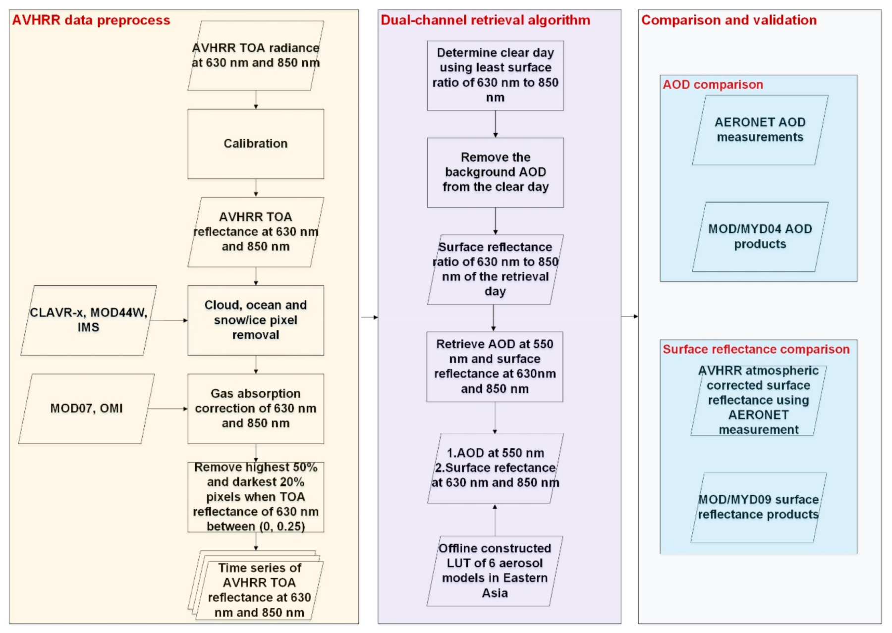
3. Retrieval Methodology

The flowchart of the dual-channel retrieval algorithm is shown in Figure 3. A brief description of the workflow is given as below.

(a) 

AVHRR data preprocess: The detailed description of calibration, the screening, and the gas absorption correction has been given in Section 2.1. Then time series of AVHRR TOA reflectance at 0.63 and 0.85 μm were prepared.

(b) 

Dual-channel retrieval algorithm: Firstly, the clear day in 31 days was searched for each pixel according to the least TOA reflectance ratio. Secondly, the background AOD and Rayleigh scattering of the clear day was removed. Next, assuming that the surface bidirectional reflectance properties do not change during the 31 days, the surface reflectance ratio of the retrieval day was obtained. Finally, the AOD values at 0.55μm and the surface reflectance values at 0.63 and 0.85 μm were retrieved using the surface reflectance ratio of the retrieval day on the basis that the surface reflectance ratio would be monotonically decreasing as the AOD value increases. Detailed description of the algorithm is shown in Section 3.4.

(c) 

Comparison and validation: The retrieved AOD and surface reflectance results are evaluated in terms of statistical comparisons and spatial analysis of one-day case (shown in Section 4).

This part begins with the forward sensitivity analysis and the need for a dual-channel algorithm is derived. After that, the reason for choosing the surface reflectance ratio to address the BRDF effect is demonstrated theoretically in Section 3.2. Next, the whole dual-channel retrieval algorithm is stated in detail in Section 3.3 and Section 3.4. Then the uncertainty analysis was studied in Section 3.5.

3.1. Forward Sensitivity Study and the Need for a Dual-Channel AOD Algorithm

The TOA reflectance values at 0.63 and 0.85 μm were simulated as a function of AOD and the surface reflectance values at 0.63 and 0.85 μm using the 6SV software [41]. The two sets of the surface reflectance values at 0.85 μm (0.15 and 0.2) were used, each one of which was assumed with two different surface reflectance ratios between 0.63 and 0.85 μm ($k^{\prime }$ = 0.1177, 0.845). The solar zenith angle is 22.14°, the satellite zenith angle is 48°, and the relative azimuth angle −156.41°. Figure 4 shows that under some condition, only using 0.63 μm channel to retrieve AOD may cause larger error than using both channels at 0.63 and 0.85 μm. For example, when $k^{\prime }$ = 0.1177, two TOA reflectance lines of 0.63 μm are too close to each other so that it is difficult to accurately extract AOD value from the TOA reflectance values, especially when AOD value is high. To depict the surface reflectance ratio $k^{\prime }$ in such condition, we simulated the TOA reflectance ratio of 0.63 to 0.85 μm as the function of AOD using 6SV software [41] (the relationship is shown in Figure 5). Overall, four groups of surface reflectance values at 0.63 and 0.85 μm were used at the same values of Figure 4. The sun-view angles were also taken the same values. It can be shown that using $k^{\prime }$ instead of the surface reflectance at 0.63 μm can help differentiate two indistinguishable lines in Figure 4 when $k^{\prime }$ = 0.1177. The two lines can be distinguished more easily as the AOD value increases. Therefore, it is necessary to use the measurements of two AVHRR red and near-infrared channels in order to retrieve accurate AOD values. It should also be noted that in Figure 4 when surface reflectance value at 0.85 μm is 0.2 the TOA reflectance value decreases with the increasing AOD. This is contrary to the assumption based on which the clear day is selected and should be avoided in the AOD retrieval.

In order to further illustrate the different sensitivities of AOD inversion between using the conventional 0.63 μm channel and using the $k^{\prime }$ ratio in the case of $k^{\prime }$ = 0.1177, the AOD values at 0.55 μm were retrieved with errors added to the surface reflectance at 0.63 μm and to the $k^{\prime }$ ratio, respectively. Errors ranging from −0.05 to 0.05 stepped by 0.01 were used. In the forward simulation the surface reflectance at 0.85 μm was set as 0.15 and the $k^{\prime }$ value of 0.1177 was used. The sun-view angles were the same as Figure 4 and Figure 5. It is shown that the AOD mean absolute error (MAE) of the conventional algorithm is much larger than that of the dual-channel algorithm (Figure 6). Therefore, the AOD retrieval algorithm using the $k^{\prime }$ ratio is more robust to the input error than the conventional 0.63 μm-channel algorithm. The founding illustrates that under some condition using the 0.63 μm channel alone to retrieve AOD may be inadequate and cause large error.

The effect of the $k^{\prime }$ ratio error on the discrimination of the TOA reflectance ratios was also investigated. The sun-view angles and the surface reflectance values at 0.85 μm were taken the same values as Figure 4 and Figure 5. The error of ±0.05 and ±0.1 was added to the $k^{\prime }$ value (depicted in Figure 7 and Figure 8, respectively). It is shown that for $k^{\prime }$ = 0.845 the error of ±0.05 would cause the TOA reflectance ratio indistinguishable, while for $k^{\prime }$ = 0.1177 the condition varies with the AOD value. When the AOD value is less than 1, the error of ±0.05 would cause the TOA reflectance ratio difficult to be distinguished (Figure 7). When the AOD value is larger than 1, the error of the $k^{\prime }$ value causing the TOA reflectance ratio indistinguishable would be 0.1 (Figure 8).

3.2. Why Choosing the Surface Reflectance Ratio to Address the BRDF Effect?

Beside the above forward sensitivity study, the reason for choosing the surface reflectance ratio to address the BRDF effect due to the view geometry variation and solar angular change is also demonstrated from the theoretical point of view followingly.

Previous studies have shown that the surface bidirectional reflectance properties can be described by two parts that vary separately with wavelength and geometry [45]. Moreover, the scale of surface geometrical structure considering the shadowing effects is much larger than the wavelength [45]. Therefore, the surface reflectance shape can be assumed as independent of the wavelength [46]. Furthermore, the surface bidirectional reflectance $A_{\mathsf{\Omega },\lambda }$ can be described as the product of the surface reflectance magnitude and the surface reflectance shape [47].

$$A_{\mathsf{\Omega },\lambda }=f_{\lambda , t}\times B_{\mathsf{\Omega }}$$

(2)

where $f_{\lambda , t}$ is the surface reflectance magnitude varying with the wavelength $\lambda$ and time, $B_{\mathsf{\Omega }}$ is the surface reflectance shape mainly depending on the geometry $\mathsf{\Omega }$. $B_{\mathsf{\Omega }}$ can be assumed as varying much more slowly than the surface reflectance magnitude [47].

Then the following ratio was used [48,49] to address the surface reflectance issue in AOD retrieval as follows.

$$k_{\lambda }=\frac{A_{{\mathsf{\Omega }}_1,\lambda }}{A_{{\mathsf{\Omega }}_2,\lambda }}\approx k,$$

(3)

Herein, Equation (3) is transformed to more conveniently relate the surface bidirectional reflectance of the retrieval day to that of the clear day. The transformation is

$$k_{\mathsf{\Omega }}^{\prime }=\frac{A_{\mathsf{\Omega },{\lambda }_1}}{A_{\mathsf{\Omega },{\lambda }_2}},$$

(4)

From Equations (2) and (3), we can obtain

$$\begin{array}{cc}{k}_{{\lambda }_1}-k_{{\lambda }_2}=\frac{A_{{\mathsf{\Omega }}_1,{\lambda }_1}}{A_{{\mathsf{\Omega }}_2,{\lambda }_1}}& -\frac{A_{{\mathsf{\Omega }}_1,{\lambda }_2}}{A_{{\mathsf{\Omega }}_2,{\lambda }_2}}=\left(\frac{f_{{\lambda }_1,t_1}}{f_{{\lambda }_1,t_2}}-\frac{f_{{\lambda }_2,t_1}}{f_{{\lambda }_2,t_2}}\right)\times \frac{B_{{\mathsf{\Omega }}_1}}{B_{{\mathsf{\Omega }}_2}}\\ & =\frac{f_{{\lambda }_1,t_1}\times f_{{\lambda }_2,t_2}-f_{{\lambda }_2,t_1}\times f_{{\lambda }_1,t_2}}{f_{{\lambda }_1,t_2}\times f_{{\lambda }_2,t_2}}\times \frac{B_{{\mathsf{\Omega }}_1}}{B_{{\mathsf{\Omega }}_2}}\end{array}$$

(5)

Because $B_{\mathsf{\Omega }}$ is assumed as varying much more slowly than the surface reflectance magnitude [47], Equation (5) can be simplified as

$$k_{{\lambda }_1}-k_{{\lambda }_2}\approx \frac{f_{{\lambda }_1,t_1}\times f_{{\lambda }_2,t_2}-f_{{\lambda }_2,t_1}\times f_{{\lambda }_1,t_2}}{f_{{\lambda }_1,t_2}\times f_{{\lambda }_2,t_2}}=\frac{f_{{\lambda }_1,t_1}}{f_{{\lambda }_1,t_2}}-\frac{f_{{\lambda }_2,t_1}}{f_{{\lambda }_2,t_2}}$$

(6)

When ${\lambda }_1$ and ${\lambda }_2$ take the red and near-infrared bands, respectively, the quantity of $k_{{\lambda }_1}-k_{{\lambda }_2}$ can be considerable, as for the soybeans, savannah and pasture land (Figure 9). However, if we substitute the denominator of the right part of Equation (6) for $f_{{\lambda }_2,t_1}\cdot f_{{\lambda }_2,t_2}$, we can obtain

$$\begin{gathered} \frac{f_{{\lambda }_1,t_1}\times f_{{\lambda }_2,t_2}-f_{{\lambda }_2,t_1}\times f_{{\lambda }_1,t_2}}{f_{{\lambda }_2,t_1}\times f_{{\lambda }_2,t_2}}=\frac{f_{{\lambda }_1,t_1}}{f_{{\lambda }_2,t_1}}-\frac{f_{{\lambda }_1,t_2}}{f_{{\lambda }_2,t_2}}=\frac{f_{{\lambda }_1,t_1}}{f_{{\lambda }_2,t_1}}\times \frac{B_{{\mathsf{\Omega }}_1}}{B_{{\mathsf{\Omega }}_1}}-\frac{f_{{\lambda }_1,t_2}}{f_{{\lambda }_2,t_2}}\times \frac{B_{{\mathsf{\Omega }}_2}}{B_{{\mathsf{\Omega }}_2}} \\ =\frac{A_{{\mathsf{\Omega }}_1,{\lambda }_1}}{A_{{\mathsf{\Omega }}_1,{\lambda }_2}}-\frac{A_{{\mathsf{\Omega }}_2,{\lambda }_1}}{A_{{\mathsf{\Omega }}_2,{\lambda }_2}}=k_{{\mathsf{\Omega }}_1}^{\prime }-k_{{\mathsf{\Omega }}_2}^{\prime } \end{gathered}$$

(7)

Equation (7) is generally smaller than Equation (6) because $f_{{\lambda }_2,t_1}$ is usually much larger than $f_{{\lambda }_1,t_2}$. Therefore, it is more reasonable to assume that the surface reflectance ratio $k^{\prime }$ remains unchanged during a certain period of time compared to $k_{\lambda }$ (Equation (3)).

$$k_{t_1}^{\prime }=k_{t_2}^{\prime }=\cdots =k^{\prime },$$

(8)

Followingly, the Rahman–Pinty–Verstraete (RPV) model [50] was used to verify the validity of Equation (8). The RPV model was developed through taking the hot spot effect into consideration on the basis of earlier empirical bidirectional reflectance models. A total of three input parameters are required in the model. Rahman et al. [50] has listed a set of inversion results of the three parameters for different cover types in the AVHRR red and near-infrared channel against various datasets, including ground-based, laboratory, and airborne measurements (Table 1 in the RPV paper). The inversion results were used in the analysis. The hard wheat type was excluded for possible printing error because the surface reflectance values of the hard wheat are different from those in the original data source [51]. The validity of Equation (8) was analyzed as follows. Firstly, the geometries of the test were from the same location at which 15 AVHRR images from 14 June 2009 to 28 June 2009 onboard the NOAA-19 satellite were taken. Secondly, the surface reflectance values were calculated from the RPV model using the above geometries and $k^{\prime }$ ($k$) values were obtained. Then, the difference of any two $k^{\prime }$ ($k$) values was calculated. Lastly, all the difference values of $k^{\prime }$ ($k$) were averaged to obtain the MAE of $k_{{\mathsf{\Omega }}_1}^{\prime }-k_{{\mathsf{\Omega }}_2}^{\prime }$ and $k_{{\lambda }_1}-k_{{\lambda }_2}$ for different ground cover types (shown in Figure 9). ${\lambda }_1$ and ${\lambda }_2$ was taken as the red and near-infrared channel, respectively. A smaller difference means more robustness on geometry. The mean absolute error of $k_{{\mathsf{\Omega }}_1}^{\prime }-k_{{\mathsf{\Omega }}_2}^{\prime }$ is 0.015 while that of $k_{{\lambda }_1}-k_{{\lambda }_2}$ 0.1. $k_{{\mathsf{\Omega }}_1}^{\prime }-k_{{\mathsf{\Omega }}_2}^{\prime }$ is much smaller than $k_{{\lambda }_1}-k_{{\lambda }_2}$. Verification with the RPV model demonstrates the improvement of Equation (8) when applied to the red and near-infrared channels. Furthermore, by addressing the unignorable BRDF issue through the $k^{\prime }$ ratio, the AOD retrievals could be improved not only because the more reasonable assumption of the unchanged $k^{\prime }$ ratio during a certain period of time than the tradition ratio $k$, but also because the AOD retrieval using the $k^{\prime }$ ratio is more robust to the error than the conventional algorithm (Figure 6).

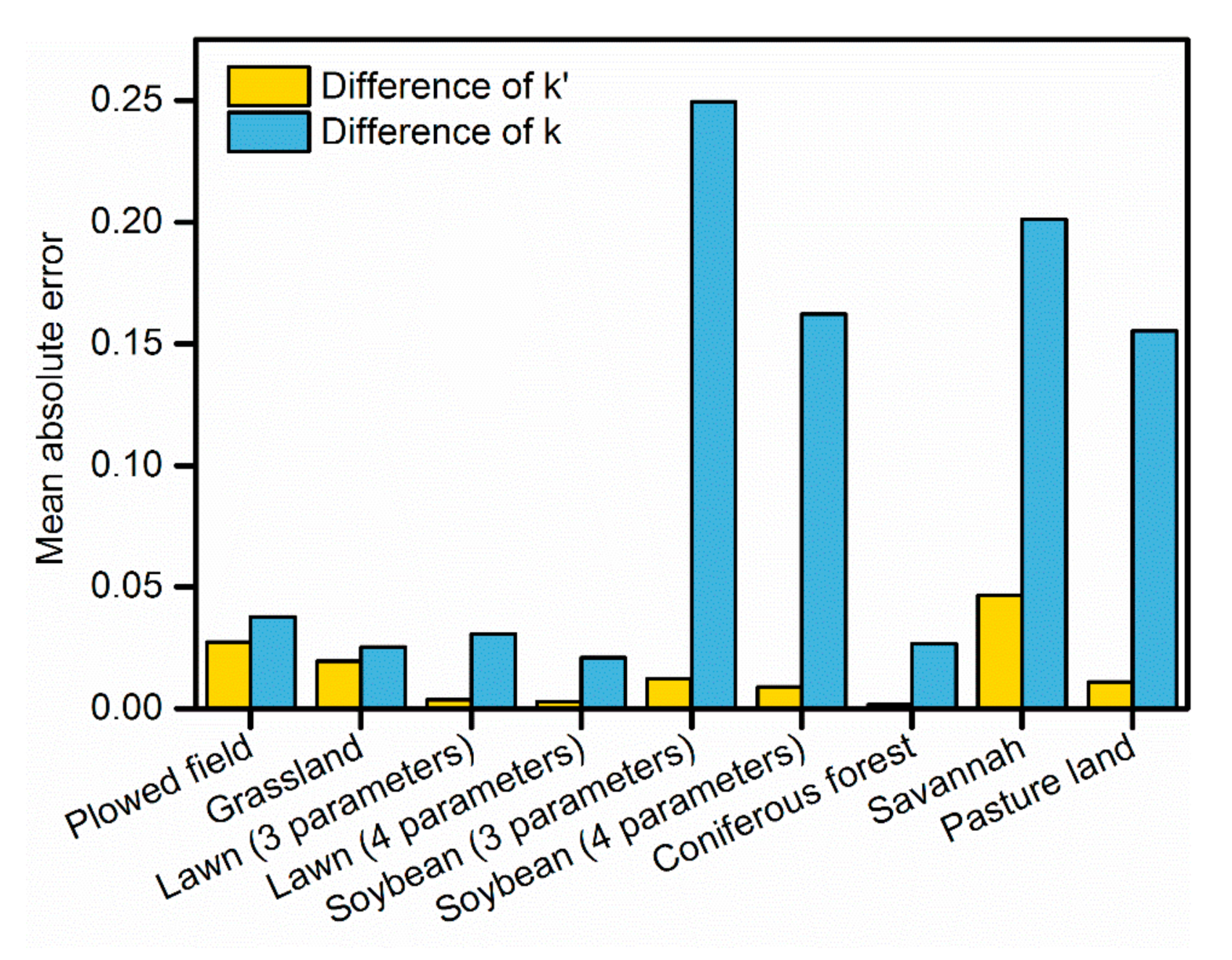
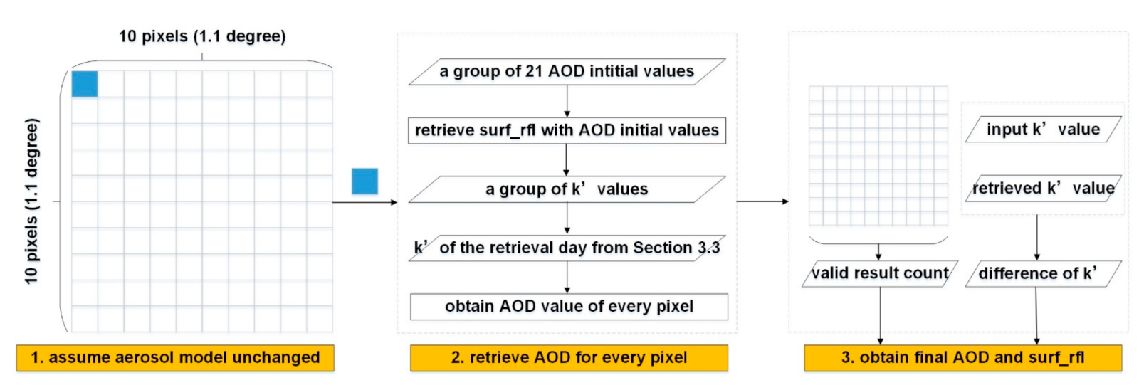
3.3. Determination of the Surface Reflectance Ratio $k^{\prime }$

After the AVHRR data preprocess, the clear day was searched by pixel from ±15 days of the retrieval image with the assumptions that the surface bidirectional properties do not change in 31 days and that at least one clear day exists in the 31-day span. The 31-day span was selected because too long a time period may have a significant surface reflectance change. For the contrasting too short a time period there might be no enough cloud clear days to select and the retrieved AOD values may be lower than the ground measurements [22,52]. The retrieval region was confined to non-bright areas where NDVI is greater than 0.15. Then, the clear day was determined by the least TOA reflectance ratio of 0.63 to 0.85 μm because the atmospheric effect would increase the TOA reflectance at 0.63 μm and decrease the TOA reflectance at 0.85 μm in the non-bright areas.

After the clear day was found, the surface reflectance at 0.63 and 0.85 μm of the clear day can be acquired via removing the background AOD and Rayleigh scattering. Knapp et al. [53] demonstrated that the background AOD value error can be introduced to AOD retrieval, but the error is not enlarged in AOD retrievals. In this study, daily Aqua MODIS Deep Blue AOD product (MYD08_D3 Version 6.1) was averaged to produce monthly background AOD values, similar to Hsu et al. [22]. Then, the surface reflectance ratio $k^{\prime }$ of the clear day pixel was determined according to Equation (4). Assuming the surface bidirectional reflectance properties do not change during a period of time, the surface ratio $k^{\prime }$ of the retrieval day can be derived according to Equation (8).

3.4. The Dual-Channel AOD Retrieval Algorithm

The flowchart of the AOD retrieval algorithm after the determination of the surface reflectance ratio $k^{\prime }$ is shown in Figure 10. The AVHRR AOD value was retrieved in the 10 × 10 pixels aggregation box (1.1 degree × 1.1 degree). In the box, aerosol model was treated as unchanged [54] assuming that aerosol optical properties change slowly in space [55]. The six aerosol models in Eastern Asia clustered from ground-based measurements [56] were used. Then for every aerosol model in each box, the AOD spatial distribution was retrieved by the following steps. Firstly, a group of 21 AOD initial values (0.05, 0.1, 0.15, 0.2, 0.3, 0.4, 0.5, 0.6, 0.7, 0.8, 0.9, 1.0, 1.25, 1.5, 2, 2.5, 3, 3.5, 4, 4.5, and 5) were constructed. Then for each AOD initial value, the surface reflectance value at 0.63 and 0.85 μm was retrieved by linear interpolation using the 6SV-calculated Lookup Table (LUT; the 6SV software cf. [41]). In the LUT, the TOA reflectance at 0.63 and 0.85 μm was calculated offline as a function of solar zenith angle, satellite zenith angle, relative azimuth angle, AOD, surface reflectance, and aerosol model. Detailed description of the LUT is shown in

Table 3. Dimensions of the LUT for aerosol retrieval.

Variable Name	No. of Entries	Entries
Wavelength (μm)	2	0.63, 0.85
Solar zenith angle (°)	8	0, 12, 24, 36, 48, 54, 60, 66
Satellite zenith angle (°)	11	0, 8, 14, 20, 24, 30, 36, 42, 48, 54, 60
Relative azimuth angle (°)	15	0, 12, 24, 36, 48, 60, 72, 84, 96, 108, 120, 132, 144, 160, 180
AOD	5	0.0001, 0.25, 0.5, 1.0, 2.0, 3.0, 4.0
Surface reflectance	7	0.01, 0.12, 0.15, 0.18, 0.23, 0.34, 0.45
Aerosol model	6	from [55]

. Therefore, the group of surface reflectance ratio $k^{\prime }$ (having 21 values corresponding to the AOD initial values) was obtained.

It followed that the $k^{\prime }$ group was compared with the surface reflectance ratio $k^{\prime }$ of the retrieval day determined from Section 3.3 to obtain AOD value at 0.55 μm by linear interpolation. The basis for this step is that $k^{\prime }$ would be monotonically decreasing as the AOD value increases. It is because for given surface reflectance values at 0.63 and 0.85 μm, the atmospheric effect would increase the TOA reflectance at 0.63 μm and decrease the TOA reflectance at 0.85 μm in the non-bright areas. Therefore, when the TOA reflectance values are given, the surface reflectance value at 0.63 μm will decrease with the increasing AOD values, while the surface reflectance value at 0.85 μm will increase. Thus, the ratio $k^{\prime }$ between 0.63 and 0.85 μm would be monotonically decreasing as the AOD value increases. If we draw a horizonal line near around 0.8 in the Figure 5, it is also shown that when the TOA reflectance ratio is given (~0.8), the AOD value increases with the decreasing surface reflectance ratio (k′) value (from 0.845 to 0.1177).

Lastly, the final AOD value at 0.55 μm and surface reflectance value at 0.63 and 0.85 μm of every box were retrieved according to the valid result count in the box and the least difference between the retrieved and input surface reflectance ratios. It is noted that the spatial resolution of retrieved AOD and surface reflectance is 11 km.

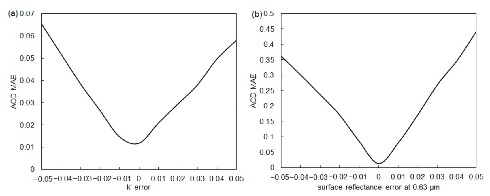
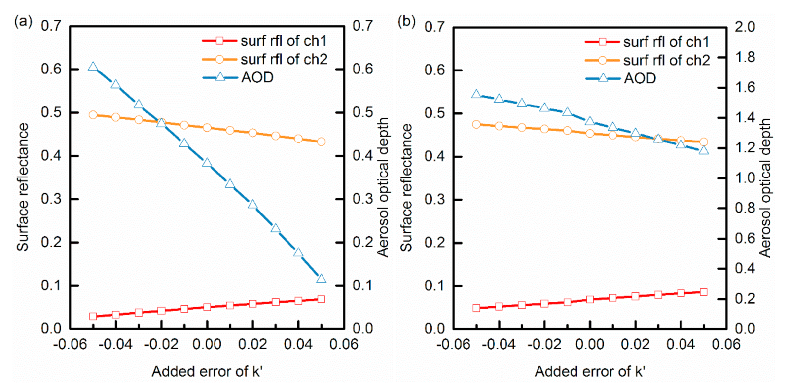
3.5. Uncertainty Study

AOD retrievals with different added errors of $k^{\prime }$ were simulated in this part. Errors ranging from −0.05 to 0.05 stepped by 0.01 were added to the surface ratio $k^{\prime }$. The value of 0.05 was used because the differences of $k^{\prime }$ for most ground cover types are less than 0.05 as shown in Figure 9. The sun-view angles were the same as Figure 4 and Figure 5. The AOD value was set as 0.4 and 1.5, respectively. A typical vegetation example is shown (the surface reflectance at 0.63and 0.85 μm is 0.05 and 0.46, respectively) in Figure 11. It is revealed that the surface reflectance value at 0.85 μm decreases slowly, whereas the AOD value decreases as the surface reflectance value at 0.63 μm increases. It should be noted that the surface reflectance input at 0.63 μm is much less than that at 0.85 μm. It implies that the $k^{\prime }$ error has a larger effect on the surface reflectance at 0.63 μm than on the surface reflectance at 0.85 μm. When the AOD value is 0.4 and 1.5, the maximum relative errors of AOD are 71.4 and 21.3%, respectively (The relative error ${\delta }_{\tau }$ of AOD is defined as ${\delta }_{\tau }=\frac{\tau -{\tau }_{\mathrm{ref}}}{{\tau }_{\mathrm{ref}}}$, here ${\tau }_{\mathrm{ref}}$ represents the reference value of $\tau$ and as to Figure 11a,b ${\tau }_{\mathrm{ref}}$ is 0.4 and 1.5, respectively). Therefore, it is indicated that the accuracy of $k^{\prime }$ has a greater impact on the AOD retrieval when the AOD value is low.

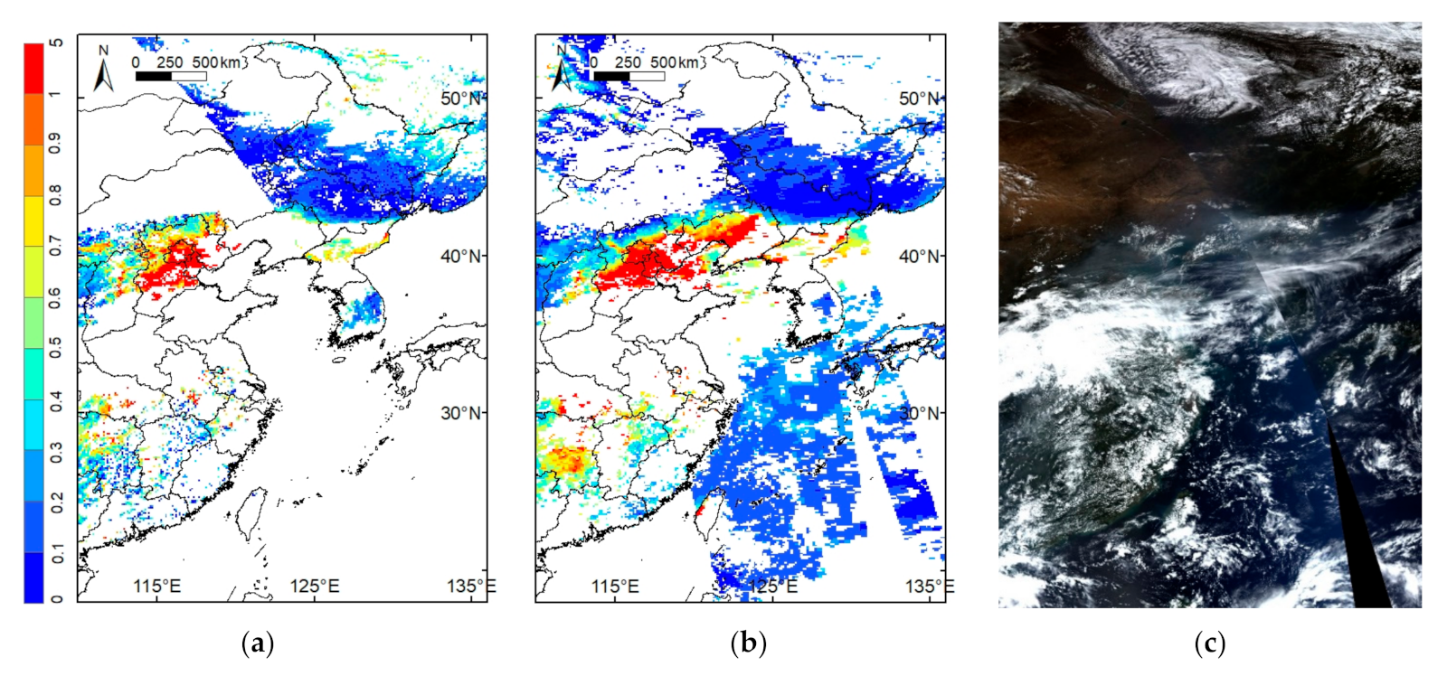
4. Results and Validation

First, the retrieved surface reflectance value was compared with the atmospherically corrected surface reflectance value using AERONET observation and MOD09 product. Then, the retrieved AOD value was compared with AERONET observation and MODIS AOD value. The spatial distribution of one day is also shown.

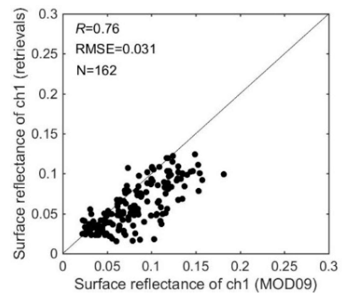
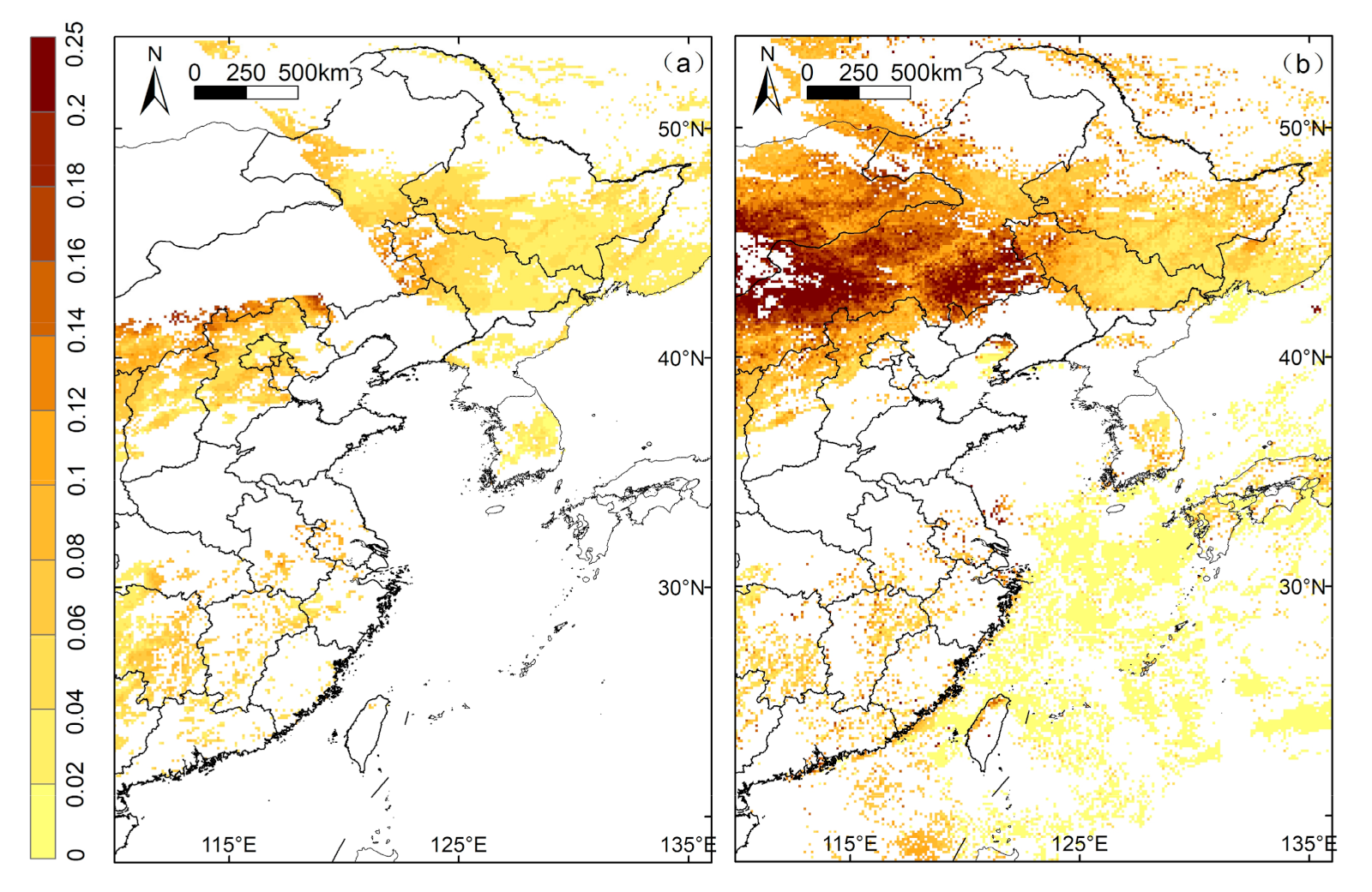
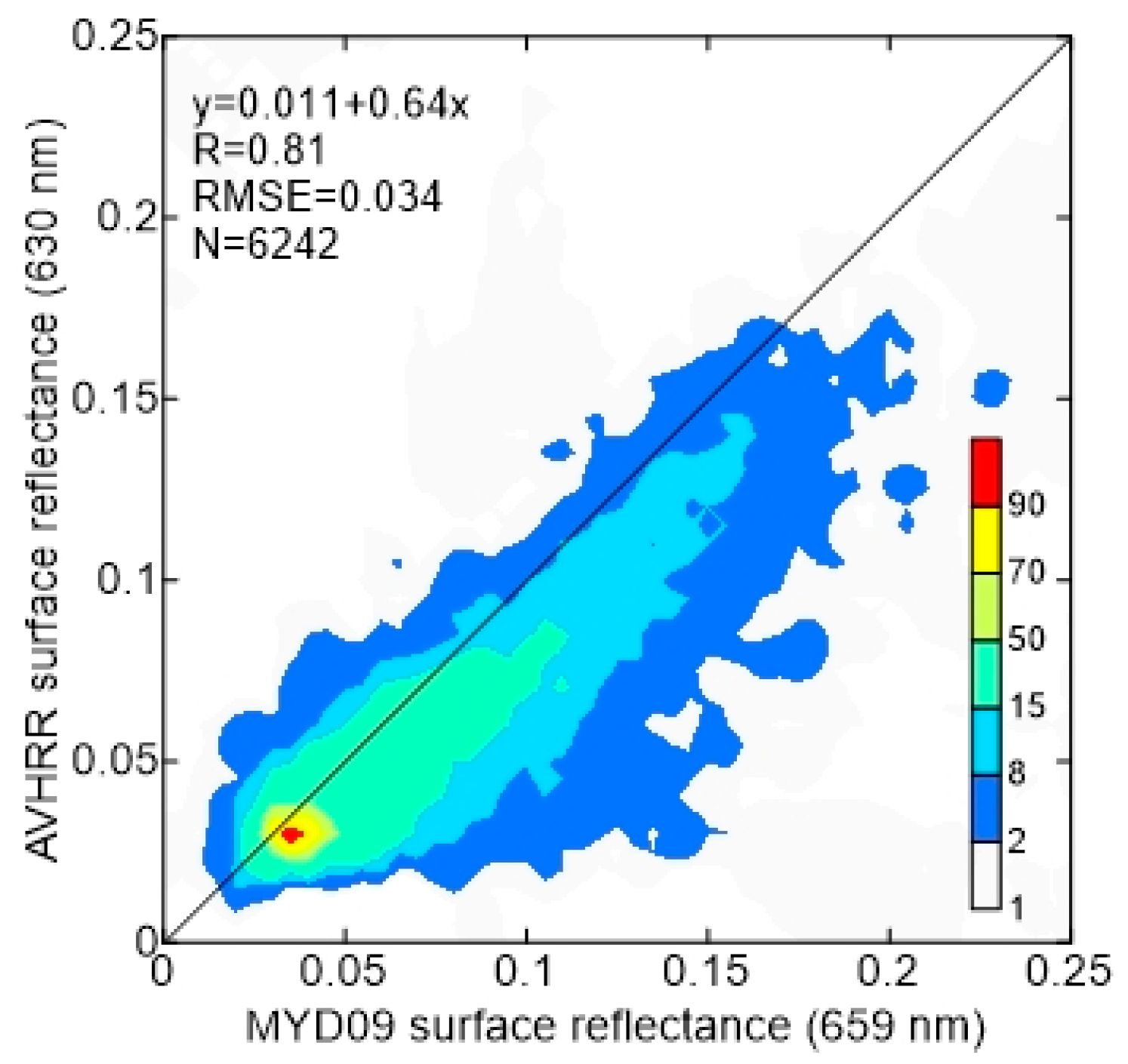
4.1. Comparison of the Retrieved Surface Reflectance against Atmospherically Corrected Surface Reflectance and MOD09 Product

The retrieved surface reflectance value was compared with the AVHRR atmospheric-corrected surface reflectance value first. The AVHRR atmospheric-corrected surface reflectance was derived with the input of the ground-based AERONET AOD, size distribution, and complex refractive index product and can be considered as benchmark surface reflectance. Figure 12 is the comparison of the surface reflectance at 0.63 and 0.85 μm. The comparison collocations of 0.63 μm shows a more dispersed distribution ($R$ = 0.59) than that of 0.85 μm. It could be caused by the estimated $k^{\prime }$ error, confirming that the $k^{\prime }$ error has a larger effect on the surface reflectance at 0.63 μm than on the surface reflectance at 0.85 μm. Furthermore, the undetected cloud and cloud shadow would intensify this error. The root mean square error (RMSE) of 0.63 and 0.85 μm is 0.03 and 0.029, respectively, also indicating the surface reflectance retrieval at 0.85 μm is more robust than that at 0.63 μm which is consistent with the uncertainty conclusion in Section 3.5.

Next, the AVHRR surface reflectance retrieval was compared with daily Terra and Aqua MODIS MOD09GA surface reflectance product of a 500 m spatial resolution in the AERONET stations. The AVHRR channel 1 result of the morning satellite (NM) was compared with the MOD09GA channel 1 result of Terra satellite, while the AVHRR result of the afternoon satellites (NN and NP) was compared with the MYD09GA result of Aqua satellite. The channel 2 result was not used for comparison because the spectral response curve of channel 2 of AVHRR is much wider than that of MODIS (Figure 2). The MOD09GA result which is identified with cloud pollution was removed. The correlation coefficient $R$ of channel 1 is 0.76, and the RMSE error 0.031 (Figure 13). The AVHRR channel 1 surface reflectance is generally less than the MODIS surface reflectance. The difference would be caused by the different spectral response functions between the AVHRR and MODIS bands (Figure 2). The comparison between AVHRR and MOD09GA surface reflectance results shows that the alignment between the two surface reflectance results is relatively good.

Figure 14 shows a comparison map example of AVHRR surface reflectance retrieval at 0.63 μm compared with the MYD09 surface reflectance product at 0.66 μm on 24 September 2009. Note that the AVHRR algorithm is applicable to non-bright region with the exception of oceans. The scatter-density plot shows similar performance between the AVHRR and MYD09 surface reflectance products with the $R$ 0.81 and the RMSE error 0.034 (Figure 15). The lower AVHRR surface reflectance values than MODIS would be due to the different spectral response functions between the AVHRR and MODIS bands.

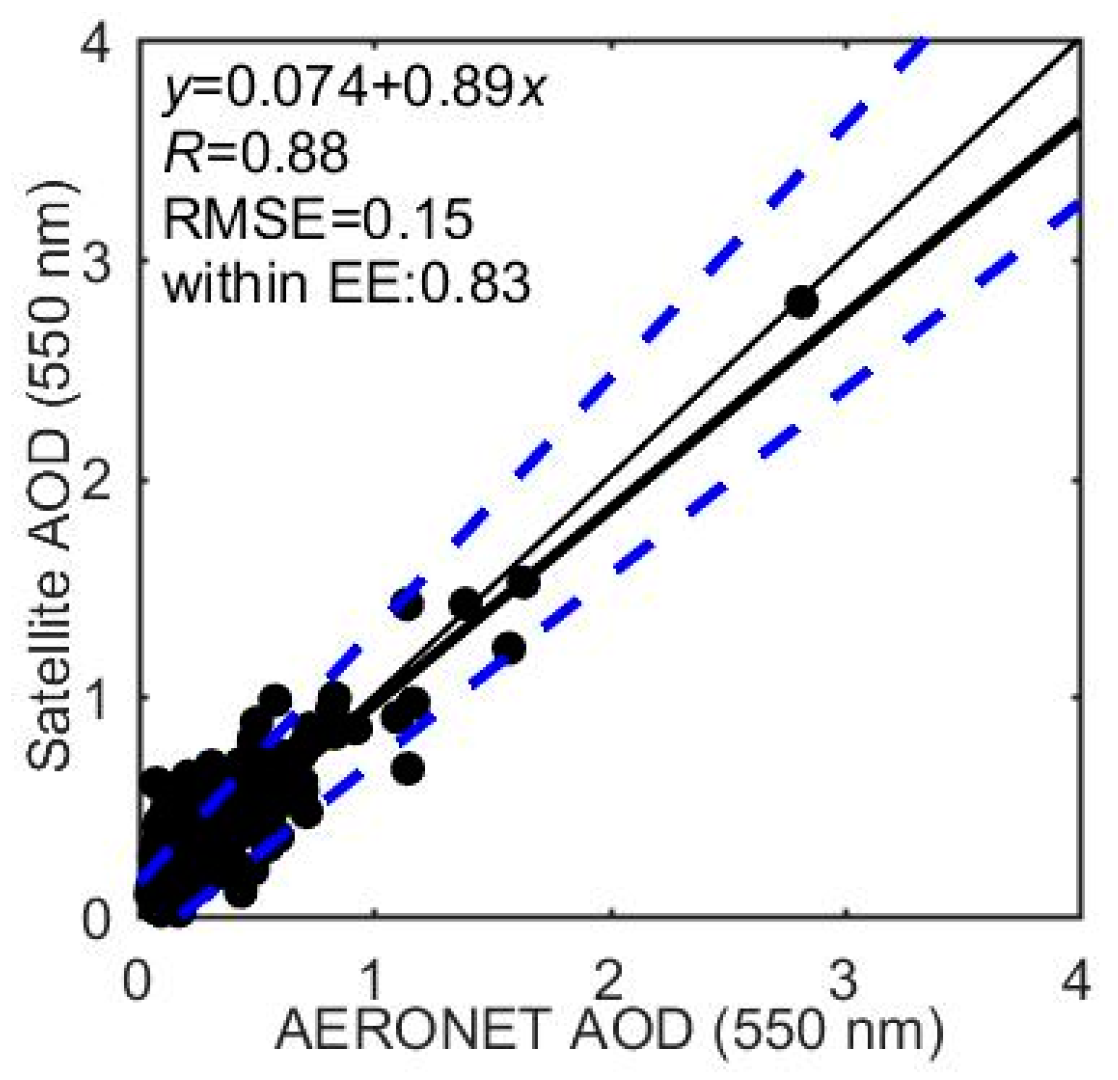
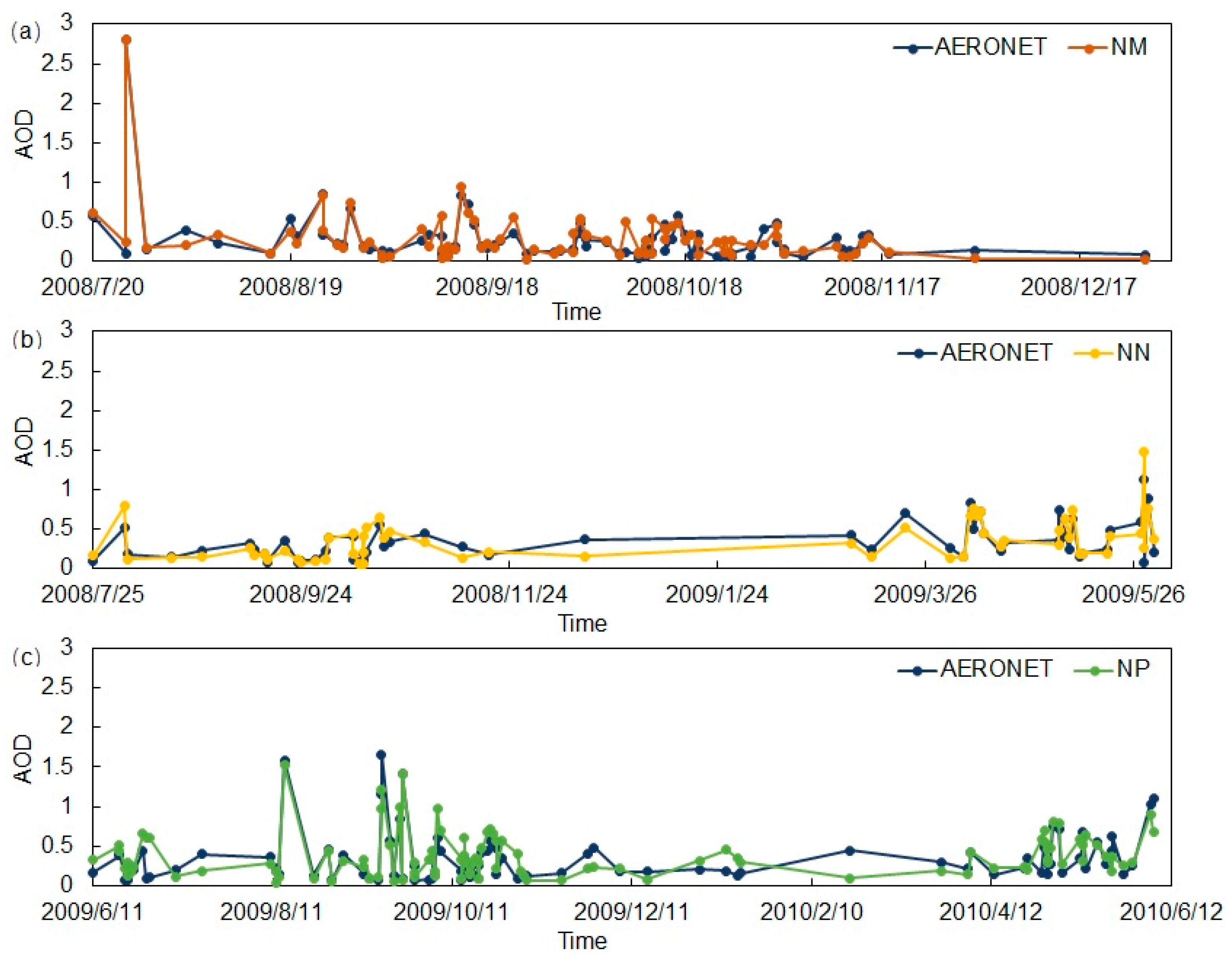
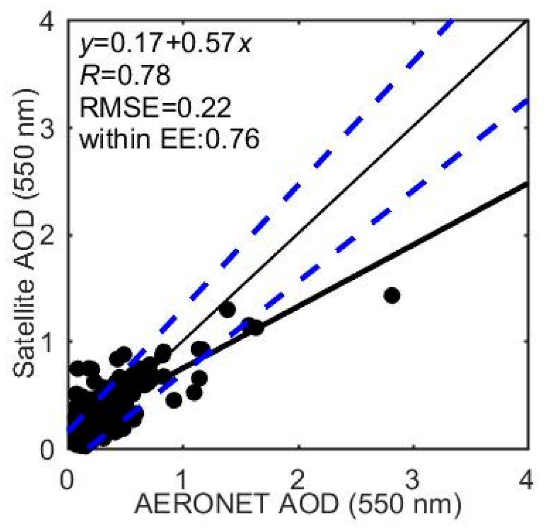
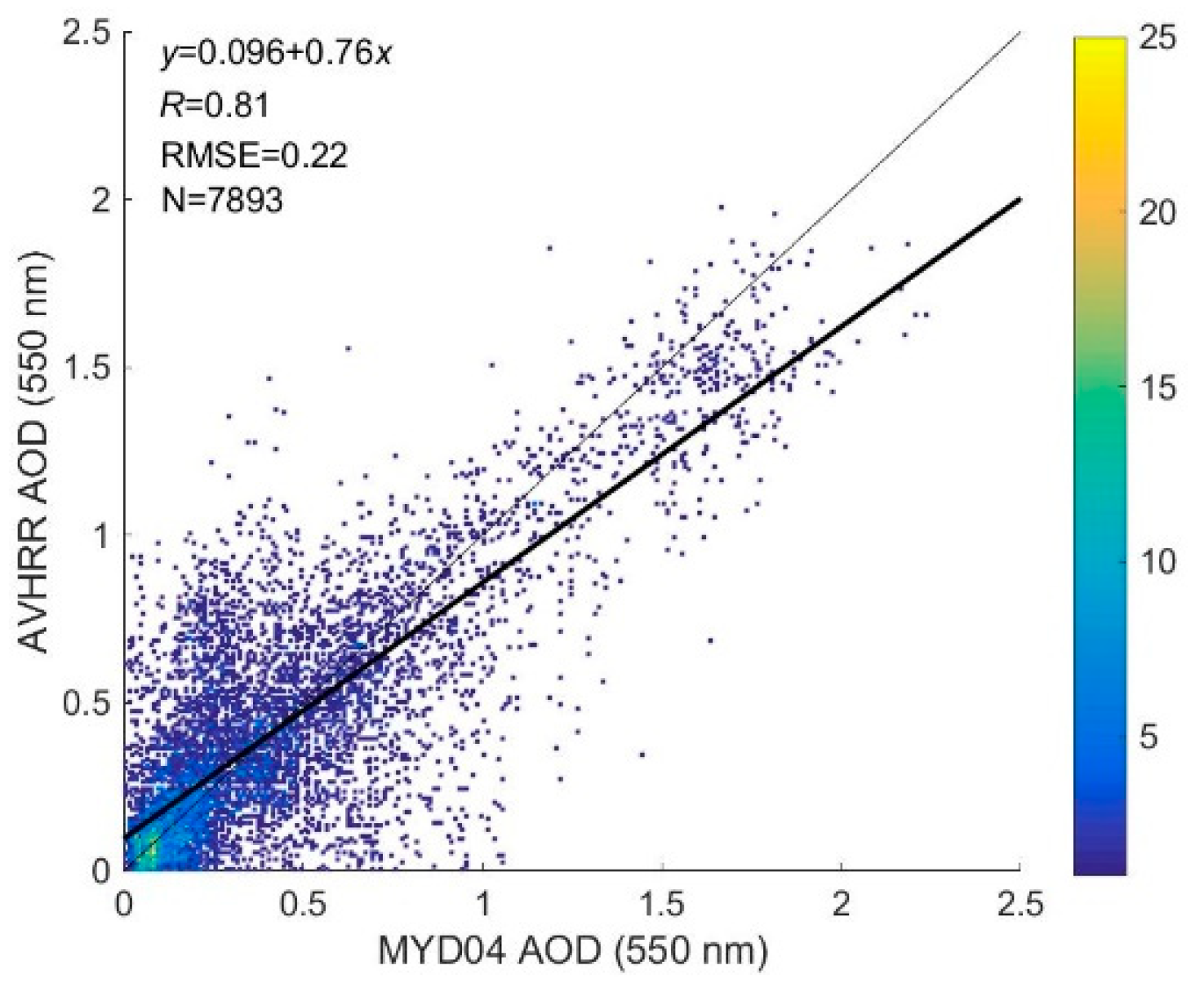
4.2. Comparison of the AOD Retrieval against the AERONET and MODIS Products

We compared the derived AVHRR AOD result with the AERONET data and MODIS product taking the spatiotemporal effect into consideration. A mean AERONET observation within ±30 min of the satellite overpass was calculated so that it could be compared with the mean of 5 × 5 pixels centered over the AERONET station [44]. The result is considered as valid if half of the pixels have values.

Figure 16 depicts the relationship between the AVHRR AOD value and AERONET AOD observation at 0.55 μm, yielding the linear regression equation of $y$ = 0.074 + 0.89$x$ with an $R$ of 0.88, an RMSE of 0.15, and 83% of collocations within error lines (±0.15 ± 0.15$\tau$, $\tau$ is AOD). The non-zero intercept may be attributed to the calibration inaccuracies or the surface tackling error, and the deviation of the slopes from unity results from the inappropriate selection of aerosol model in the AVHRR algorithm [44]. The RMSE error is probably due to the random error caused by the surface reflectance changes or subpixel cloud contamination, while the $R$ denotes the possible ability to detect aerosol signal from the AVHRR sensor [22,57,58,59,60].

Time series comparison of AVHRR AOD retrievals versus AERONET AOD measurements within ±30 min of the satellite overpass is shown in Figure 17. The three AVHRR onboard satellites were involved, namely NM, NN, and NP. It is shown that the AVHRR AOD retrievals can capture the AOD changes over time.

The conventional estimate of AOD at 0.55 μm using 0.63 μm channel was also retrieved. The conventional estimate of AOD used the same clear day results as the $k^{\prime }$ ratio. Validation against the AEROENT measurement in Figure 18 shows that the linear regression equation is $y$ = 0.17 + 0.57$x$ with an $R$ of 0.78 and an RMSE error of 0.22, which is inferior to the AOD retrieval using the $k^{\prime }$ ratio.

One example of the large-scale AOD retrievals from AVHRR and MODIS is shown in Figure 19. Both the AQUA/MODIS Dark Target and Deep Blue AOD products are utilized. The AVHRR AOD spatial distribution is similar to the MYD04 product, which is low in 42–54° N and high in 38–42° N covering the Beijing, Tianjin, and Hebei province, China. The AVHRR AOD retrievals at 0.55 μm on 24 September 2009 were also compared with MYD04 AOD products at 0.55 μm (Figure 20). It is shown that the linear regression line is $y$ = 0.096 + 0.76$x$ with an $R$ of 0.81 and an RMSE 0.22.

5. Conclusions

The orbit drift and phasing running of NOAA satellites and large view geometry variation would cause an unignorable BRDF effect in the determination of surface reflectance from time series of AVHRR measurements. Our forward sensitivity study found the need for dual channels at 0.63 μm and 0.85 μm to retrieve AOD instead of the single-channel algorithm using 0.63 μm. We used the surface reflectance ratio $k^{\prime }$ between 0.63 μm and 0.85 μm to address the surface BRDF effect. The ratio was demonstrated from both the forward-sensitivity and theoretical point of view and the validity was examined. It was found that the AOD inversion using the $k^{\prime }$ ratio is more robust to the input error than the conventional 0.63 μm-channel algorithm. Moreover, it is more reasonable to assume that the $k^{\prime }$ ratio remains unchanged during a certain period of time compared to the traditional ratio $k$ when addressing the BRDF issue. Then, the AVHRR dual-channel algorithm was proposed to determine AOD at 0.55 μm and surface reflectance at 0.63 and 0.85 μm. This novel approach was applied to Eastern Asia. The surface reflectance retrieval was compared with the atmospherically corrected surface reflectance value and MODIS surface reflectance product. The surface reflectance at 0.85 μm has better statistic results than that at 0.63 μm, consistent with the uncertainty conclusion. The AOD retrieval was compared with AERONET AOD observation, yielding the linear regression equation of $y$ = 0.074 + 0.89$x$ with an $R$ of 0.88, an RMSE error of 0.15. The fraction of the AOD validation collocations within the error lines (±0.15 ± 0.15$\tau$) was 83%. The favorable correlation provides confidence in the utility of our AVHRR AOD algorithm over land. Time series comparison between AVHRR AOD retrievals and AERONET AOD measurements shows that the AVHRR AOD retrievals can capture the AOD changes over time. The proposed dual-channel AOD algorithm taking into account the surface BRDF effect is proved outperforming the conventional 0.63 μm-channel method.

The generic nature of the dual-channel algorithm makes it appropriate for AOD retrievals from common sensors, especially from those that lack the shortwave infrared channel that is required in the MODIS Dark Target AOD algorithm. Nonetheless, the present algorithm is confined to non-bright regions because of the use of the clear day. Moreover, the algorithm is more suitable for the situation in which the surface reflectance does not change dramatically. Further research could focus on improving the gathering of the surface reflectance of an adjacent clear day, such as adopting the quantitative expression of surface bidirectional reflectance [46] and employing a non-Lambertian forward model [61,62].

AVHRR may provide an almost 40-year unique archive of AOD retrieval over land from the 1980s to present, during which time aerosol plays a particularly important and unclear role in the global and regional climate. To achieve this objective, more studies are still needed; for example, earlier aerosol model assumption and AOD validation without the AERONET observation available would be helpful.

References

1. Herman, B.M.; Browning, S.R. The effect of aerosols on the Earth-atmosphere albedo. J. Atmos. Sci. 1975, 32, 1430–1445. [Google Scholar] [CrossRef] [Green Version]
2. Haywood, J.M.; Ramaswamy, V.; Soden, B.J. Tropospheric aerosol climate forcing in clear-sky satellite observations over the oceans. Science 1999, 283, 1299–1303. [Google Scholar] [CrossRef] [Green Version]
3. Hatzianastassiou, N.; Matsoukas, C.; Drakakis, E.; Stackhouse, P.W., Jr.; Koepke, P.; Fotiadi, A.; Pavlakis, K.G.; Vardavas, I. The direct effect of aerosols on solar radiation based on satellite observations, reanalysis datasets, and spectral aerosol optical properties from Global Aerosol Data Set (GADS). Atmos. Chem. Phys. 2007, 7, 2585–2599. [Google Scholar] [CrossRef] [Green Version]
4. Xu, H.; Guo, J.P.; Ceamanos, X.; Roujean, J.L.; Min, M.; Carrer, D. On the influence of the diurnal variations of aerosol content to estimate direct aerosol radiative forcing using MODIS data. Atmos. Environ. 2016, 141, 186–196. [Google Scholar] [CrossRef]
5. Kaufman, Y.J.; Tanré, D.; Boucher, O. A satellite view of aerosols in the climate system. Nature 2002, 419, 215–223. [Google Scholar] [CrossRef]
6. Fan, J.; Leung, L.R.; Li, Z.; Morrison, H.; Chen, H.; Zhou, Y.; Qian, Y.; Wang, Y. Aerosol impacts on clouds and precipitation in eastern China: Results from bin and bulk microphysics. J. Geophys. Res. 2012, 117, D00K36. [Google Scholar] [CrossRef]
7. Boucher, O.; Randall, D.; Artaxo, P.; Bretherton, C.; Feingold, G.; Forster, P.; Kerminen, V.-M.; Kondo, Y.; Liao, H.; Lohmann, U.; et al. IPCC AR5 (2013) Chapter 7: Clouds and Aerosols. In Climate Change 2013: The Physical Science Basis. Contribution of Working Group I to the Fifth Assessment Report of the Intergovernmental Panel on Climate Change; Cambridge University Press: Cambridge, UK, 2013. [Google Scholar]
8. Wang, F.; Guo, J.; Zhang, J.; Huang, J.; Min, M.; Chen, T.; Liu, H.; Deng, M.; Li, X. Multi-sensor quantification of aerosol-induced variability in warm cloud properties over eastern China. Atmos. Environ. 2015, 113, 1–9. [Google Scholar] [CrossRef]
9. Guo, J.; Deng, M.; Lee, S.S.; Wang, F.; Li, Z.; Zhai, P.; Liu, H.; Lv, W.; Yao, W.; Li, X. Delaying precipitation and lightning by air pollution over the Pearl River Delta. Part I: Observational analyses. J. Geophys. Res. Atmos. 2016, 121, 6472–6488. [Google Scholar] [CrossRef]
10. Guo, J.; Liu, H.; Li, Z.; Rosenfeld, D.; Jiang, M.; Xu, W.; Jiang, J.H.; He, J.; Chen, D.; Min, M.; et al. Aerosol-induced changes in the vertical structure of precipitation: A perspective of TRMM precipitation radar. Atmos. Chem. Phys. 2018, 18, 13329–13343. [Google Scholar] [CrossRef] [Green Version]
11. Li, Z.; Lau, W.K.-M.; Ramanathan, V.; Wu, G.; Ding, Y.; Manoj, M.G.; Liu, J.; Qian, Y.; Li, J.; Zhou, T.; et al. Aerosol and Monsoon Climate Interactions over Asia. Rev. Geophys. 2016, 54, 866–929. [Google Scholar] [CrossRef]
12. Petrenko, M.; Kahn, R.; Chin, M.; Soja, A.; Kucsera, T.; Harshvardhan. The use of satellite-measured aerosol optical depth to constrain biomass burning emissions source strength in the global model GOCART. J. Geophys. Res. 2012, 117, D18212. [Google Scholar] [CrossRef] [Green Version]
13. Guo, J.P.; Zhang, X.Y.; Wu, Y.R.; Zhaxi, Y.; Che, H.Z.; La, B.; Wang, W.; Li, X.W. Spatio-temporal variation trends of satellite-based aerosol optical depth in China during 1980–2008. Atmos. Environ. 2011, 45, 6802–6811. [Google Scholar] [CrossRef]
14. De Leeuw, G.; Sogacheva, L.; Rodriguez, E.; Kourtidis, K.; Georgoulias, A.K.; Alexandri, G.; Amiridis, V.; Proestakis, E.; Marinou, E.; Xue, Y.; et al. Two decades of satellite observations of AOD over mainland China using ATSR-2, AATSR and MODIS/Terra: Data set evaluation and large-scale patterns. Atmos. Chem. Phys. 2018, 18, 1573–1592. [Google Scholar] [CrossRef] [Green Version]
15. Holben, B.N.; Eck, T.F.; Slutsker, I.; Tanré, D.; Buis, J.P.; Setzer, A.W.; Vermote, E.F.; Reagan, J.A.; Kaufman, Y.J.; Nakajima, T.; et al. AERONET—A federated instrument network and data archive for aerosol characterization. Remote Sens. Environ. 1998, 66, 1–16. [Google Scholar] [CrossRef]
16. Nakajima, T.; Higurashi, A. AVHRR remote sensing of aerosol optical properties in the Persian Gulf region, summer 1991. J. Geophys. Res. 1997, 102, 16935–16946. [Google Scholar] [CrossRef]
17. Higurashi, A.; Nakajima, T. Development of a Two-Channel Aerosol Retrieval Algorithm on a Global Scale Using NOAA AVHRR. J. Atmos. Sci. 1999, 56, 924–941. [Google Scholar] [CrossRef]
18. Knapp, K.R.; Stowe, L.L. Evaluating the potential for retrieving aerosol optical depth over land from AVHRR Pathfinder Atmosphere data. J. Atmos. Sci. 2002, 59, 279–293. [Google Scholar] [CrossRef]
19. Hauser, A.; Oesch, D.; Foppa, N.; Wunderle, S. NOAA AVHRR derived aerosol optical depth over land. J. Geophys. Res. 2005, 110, D08204. [Google Scholar] [CrossRef]
20. Riffler, M.; Popp, C.; Hauser, A.; Fontana, F.; Wunderle, S. Validation of a modified AVHRR aerosol optical depth retrieval algorithm over Central Europe. Atmos. Meas. Tech. 2010, 3, 1255–1270. [Google Scholar] [CrossRef] [Green Version]
21. Mei, L.; Xue, Y.; Kokhanovsky, A.A.; von Hoyningen-Huene, W.; de Leeuw, G.; Burrows, J.P. Retrieval of aerosol optical depth over land surfaces from AVHRR data. Atmos. Meas. Tech. 2014, 7, 2411–2420. [Google Scholar] [CrossRef] [Green Version]
22. Hsu, N.C.; Lee, J.; Sayer, A.M.; Carletta, N.; Chen, S.-H.; Tucker, C.J.; Holben, B.N.; Tsay, S.-C. Retrieving near-global aerosol loading over land and ocean from AVHRR. J. Geophys. Res. Atmos. 2017, 122, 9968–9989. [Google Scholar] [CrossRef] [Green Version]
23. Husar, R.B.; Prospero, J.M.; Stowe, L.L. Characterization of tropospheric aerosols over the oceans with the NOAA advanced very high resolution radiometer optical thickness operational product. J. Geophys. Res. 1997, 102, 16889–16909. [Google Scholar] [CrossRef] [Green Version]
24. King, M.D.; Kaufman, Y.J.; Tanré, D.; Nakajima, T. Remote sensing of tropospheric aerosols from space: Past, present and future. B. Am. Meteorol. Soc. 1999, 80, 2229–2259. [Google Scholar] [CrossRef] [Green Version]
25. Stowe, L.L.; Carey, R.M.; Pellegrino, P.P. Monitoring the Mt. Pinatubo aerosol layer with NOAA/11 AVHRR data. Geophys. Res. Lett. 1992, 19, 159–162. [Google Scholar] [CrossRef] [Green Version]
26. Durkee, P.A.; Pfeil, F.; Frost, E.; Shema, R. Global analysis of aerosol particle characteristics. Atmos. Environ. 1991, 25, 2457–2471. [Google Scholar] [CrossRef]
27. Ignatov, A.M.; Stowe, L.L.; Sakerin, S.M.; Korotaev, G. Validation of NOAA/NESDIS satellite aerosol product over the North Atlantic in 1989. J. Geophys. Res. 1995, 100, 5123–5132. [Google Scholar] [CrossRef]
28. Ignatov, A.M.; Stowe, L.L.; Singh, R.; Sakerin, S.; Kabanov, D.; Dergileva, I. Validation of NOAA/AVHRR aerosol retrievals using sunphotometer measurements from R/V Akademik Vernadsky in 1991. Adv. Space Res. 1995, 16, 95–98. [Google Scholar] [CrossRef]
29. Geogdzhayev, I.V.; Mishchenko, M.I. Sensitivity analysis of aerosol retrieval algorithms using two-channel satellite radiance data. Proc. SPIE 1999, 3763, 155–168. [Google Scholar]
30. Fraser, R.S.; Kaufman, Y.J.; Mahoney, R.L. Satellite measurements of aerosol mass and transport. Atmos. Environ. 1984, 18, 2577–2584. [Google Scholar] [CrossRef]
31. Kaufman, Y.J.; Fraser, R.S.; Ferrare, R.A. Satellite measurements of large-scale air pollution: Method. J. Geophys. Res. 1990, 95, 9895–9909. [Google Scholar] [CrossRef]
32. Price, J.C. Timing of NOAA afternoon passes. Int. J. Remote Sens. 1991, 12, 193–198. [Google Scholar] [CrossRef]
33. Kaufmann, R.K.; Zhou, L.; Knyazikhin, Y.; Shabanov, V.; Myneni, R.B.; Tucker, C.J. Effect of orbital drift and sensor changes on the time series of AVHRR vegetation index data. IEEE Trans. Geosci. Remote Sens. 2000, 38, 2584–2597. [Google Scholar]
34. Devasthale, A.; Karlsson, K.-G.; Quaas, J.; Grassl, H. Correcting orbital drift signal in the time series of AVHRR derived convective cloud fraction using rotated empirical orthogonal function. Atmos. Meas. Tech. 2012, 5, 267–273. [Google Scholar] [CrossRef] [Green Version]
35. McGregor, J.; Gorman, A.J. Some considerations for using AVHRR data in climatological studies: 1. Orbital characteristics of NOAA satellites. Int. J. Remote Sens. 1994, 15, 537–548. [Google Scholar] [CrossRef]
36. Gleason, A.C.R.; Prince, S.D.; Goetz, S.J.; Small, J. Effects of orbital drift on land surface temperature measured by AVHRR thermal sensors. Remote Sens. Environ. 2002, 79, 147–165. [Google Scholar] [CrossRef]
37. Heidinger, A.K.; Straka III, W.C.; Molling, C.C.; Sullivan, J.T.; Wu, X. Deriving an inter-sensor consistent calibration for the AVHRR solar reflectance data record. Int. J. Remote Sens. 2010, 31, 6493–6517. [Google Scholar] [CrossRef]
38. Molling, C.C.; Heidinger, A.K.; Straka, W.C., III; Wu, X. Calibrations for AVHRR channels 1 and 2: Review and path towards consensus. Int. J. Remote Sens. 2010, 31, 6519–6540. [Google Scholar] [CrossRef]
39. Stowe, L.L.; Davis, P.A.; Mcclain, E.P. Scientific Basis and Initial Evaluation of the CLAVR-1 Global Clear/Cloud Classification Algorithm for the Advanced Very High Resolution Radiometer. J. Atmos. Ocean Tech. 1999, 16, 656–681. [Google Scholar] [CrossRef]
40. NOAA/NESDIS/OSDPD/SSD, IMS Daily Northern Hemisphere Snow and Ice Analysis at 4 km and 24 km Resolution, Global Snow and Ice Map Datasets; National Snow and Ice Data Center: Boulder, CO, USA, 2004.
41. Vermote, E.F.; Tanré, D.; Deuzé, J.L.; Herman, M.; Morcrettte, J.-J. Second Simulation of the Satellite Signals in the Solar Spectrum, 6S: An Overview. IEEE Trans. Geosci. Remote Sens. 1997, 35, 675–686. [Google Scholar] [CrossRef] [Green Version]
42. Dubovik, O.; King, M.D. A flexible inversion algorithm for retrieval of aerosol optical properties from Sun and sky radiance measurements. J. Geophys. Res. 2000, 105, 20673–20696. [Google Scholar] [CrossRef] [Green Version]
43. Chu, D.A.; Kaufman, Y.J.; Ichoku, C.; Remer, L.A.; Tanré, D.; Holben, B.N. Validation of MODIS aerosol optical depth retrieval over land. Geophys. Res. Lett. 2002, 29. [Google Scholar] [CrossRef] [Green Version]
44. Ichoku, C.; Chu, D.A.; Mattoo, S.; Kaufman, Y.J.; Remer, L.A.; Tanré, D.; Slutsker, I.; Holben, B.N. A spatio-temporal approach for global validation and analysis of MODIS aerosol products. Geophys. Res. Lett. 2002, 29. [Google Scholar] [CrossRef] [Green Version]
45. Flowerdew, R.J.; Haigh, J.D. An approximation to improve accuracy in the derivation of surface reflectances from multi-look satellite radiometers. Geophys. Res. Lett. 1995, 22, 1693–1696. [Google Scholar] [CrossRef]
46. North, P.R.J.; Briggs, S.A.; Plummer, S.E.; Settle, J.J. Retrieval of land surface bi-directional reflectance and aerosol opacity from ATSR-2 multi-angle imagery. IEEE Trans. Geosci. Remote Sens. 1999, 37, 526–537. [Google Scholar] [CrossRef]
47. Vermote, E.; Justice, C.O.; Bréon, F.-M. Towards a Generalized Approach for Correction of the BRDF Effect in MODIS Directional Reflectances. IEEE Trans. Geosci. Remote Sens. 2009, 47, 898–908. [Google Scholar] [CrossRef]
48. Veefkind, J.P.; de Leeuw, G.; Durkee, P.A.; Russell, P.B.; Hobbs, P.V.; Livingston, J.M. Aerosol optical depth retrieval using ATSR-2 and AVHRR data during TARFOX. J. Geophys. Res. 1999, 104, 2253–2260. [Google Scholar] [CrossRef] [Green Version]
49. Tang, J.; Xue, Y.; Yu, T.; Guan, Y. Aerosol optical thickness determination by exploiting the synergy of TERRA and AQUA MODIS. Remote Sens. Environ. 2005, 94, 327–334. [Google Scholar] [CrossRef]
50. Rahman, H.; Pinty, B.; Verstraete, M.M. Coupled Surface-Atmosphere Reflectance (CSAR) Model 2. Semiempirical Surface Model Usable with NOAA Advanced Very High Resolution Radiometer Data. J. Geophys. Res. 1993, 98, 20791–20801. [Google Scholar] [CrossRef]
51. Kimes, D.; Newcomb, W.; Tucker, C.; Zonneveld, I.; Van Wijngaarden, W.; de Leeuw, J.; Epema, G. Directional reflectance factor distributions for cover types of northern Africa. Remote Sens. Environ. 1985, 18, 1–19. [Google Scholar] [CrossRef] [Green Version]
52. Knapp, K.R.; Frouin, R.; Kondragunta, S.; Prados, A. Toward aerosol optical depth retrievals over land from GOES visible radiances: Determining surface reflectance. Int. J. Remote Sens. 2005, 26, 4097–4116. [Google Scholar] [CrossRef]
53. Knapp, K.R.; Vonder Haar, T.H.; Kaufman, Y.J. Aerosol optical depth retrieval from GOES-8: Uncertainty study and retrieval validation over South America. J. Geophys. Res. 2002, 107. [Google Scholar] [CrossRef] [Green Version]
54. Mei, L.; Xue, Y.; de Leeuw, G.; Holzer-Popp, T.; Guang, J.; Li, Y.; Yang, L.; Xu, H.; Xu, X.; Li, C.; et al. Retrieval of aerosol optical depth over land based on a time series technique using MSG/SEVIRI data. Atmos. Chem. Phys. 2012, 12, 9167–9185. [Google Scholar] [CrossRef] [Green Version]
55. Li, Y.; Xue, Y.; de Leeuw, G.; Li, C.; Yang, L.; Hou, T.; Marir, F. Retrieval of aerosol optical depth and surface reflectance over land from NOAA AVHRR data. Remote Sens. Environ. 2013, 133, 1–20. [Google Scholar] [CrossRef]
56. Lee, K.H.; Kim, Y.J. Satellite remote sensing of Asian aerosols: A case study of clean, polluted, and Asian dust storm days. Atmos. Meas. Tech. 2010, 3, 1771–1784. [Google Scholar] [CrossRef] [Green Version]
57. Ignatov, A.; Stowe, L. Physical basis, premises, and self-consistency checks of aerosol retrievals from TRMM VIRS. J. Appl. Meteorol. 2000, 39, 2259–2277. [Google Scholar] [CrossRef]
58. Zhao, T.X.-P.; Stowe, L.L.; Smirnov, A.; Crosby, D.; Sapper, J.; McClain, C.R. Development of a global validation package for satellite oceanic aerosol optical thickness retrieval based on AERONET observations and its application to NOAA/NESDIS operational aerosol retrievals. J. Atmos. Sci. 2002, 59, 294–312. [Google Scholar] [CrossRef] [Green Version]
59. Zhao, T.X.-P.; Dubovik, O.; Smirnov, A.; Holben, B.N.; Sapper, J.; Pietras, C.; Voss, K.J.; Frouin, R. Regional evaluation of an advanced very high resolution radiometer (AVHRR) two-channel aerosol retrieval algorithm. J. Geophys. Res. 2004, 109, D02204. [Google Scholar] [CrossRef] [Green Version]
60. Popp, C.; Hauser, A.; Foppa, N.; Wunderle, S. Remote sensing of aerosol optical depth over central Europe from MSG-SEVIRI data and accuracy assessment with ground-based AERONET measurements. J. Geophys. Res. 2007, 112, D24S11. [Google Scholar] [CrossRef] [Green Version]
61. Li, X.; Wang, J.; Ni, W.; Strahler, A.H.; Woodcock, C. Simulation of path scattering and multiple bounces of photons between two media. Sci. China Ser. E 1996, 26, 457–466. (In Chinese) [Google Scholar]
62. Yang, L.; Xue, Y.; Jie, G.; Kazemian, H.; Zhang, J.; Li, C. Improved aerosol optical depth and Ångstrom exponent retrieval over land from MODIS based on the non-lambertian forward model. IEEE Geosci. Remote Sens. Lett. 2014, 11, 1629–1633. [Google Scholar] [CrossRef]
Figure 1. Overview of the study area and the AERONET stations.
Remotesensing 13 00365 g001
Figure 2. Normalized spectral response functions of channels 1 and 2 for AVHRR/NOAA-17-19, MODIS/Terra, and MODIS/Aqua (https://www.star.nesdis.noaa.gov/smcd/GCC/instrInfo-srf.php).
Remotesensing 13 00365 g002
Figure 3. Flowchart of the dual-channel retrieval algorithm.
Remotesensing 13 00365 g003
Figure 4. The TOA reflectance at 0.63 and 0.85 μm as the function of AOD at 0.55 μm when the solar zenith angle is 22.14°, satellite zenith angle 48°, and relative azimuth angle −156.41°. The “surf_ch2” indicates a surface reflectance at 0.85 μm. “ k = 0.1177 ( k = 0.845)” means that the surface reflectance ratio of 0.63 to 0.85 μm is 0.1177 (0.845).
Remotesensing 13 00365 g004
Figure 5. The simulated TOA reflectance ratio of 0.63 to 0.85 μm as the function of AOD at 0.55 μm when the solar zenith angle is 22.14°, satellite zenith angle 48°, and relative azimuth angle −156.41°. The “surf_ch2” indicates a surface reflectance at 0.85 μm. “ k = 0.1177 ( k = 0.845)” means that the surface reflectance ratio of 0.63 to 0.85 μm is 0.1177 (0.845).
Remotesensing 13 00365 g005
Figure 6. The AOD MAE versus the k error (a) and the surface reflectance error at 0.63 μm (b).
Remotesensing 13 00365 g006
Figure 7. The simulated TOA reflectance ratio of 0.63 to 0.85 μm as the function of AOD at 0.55 μm when the solar zenith angle is 22.14°, satellite zenith angle 48°, and relative azimuth angle −156.41°. The “surf_ch2” indicates a surface reflectance at 0.85 μm. The k value means the surface reflectance ratio of 0.63 to 0.85 μm.
Remotesensing 13 00365 g007
Figure 8. The same as Figure 7 but for different k values.
Remotesensing 13 00365 g008
Figure 9. The mean absolute errors of k Ω 1 k Ω 2 and k λ 1 k λ 2 for different ground cover types.
Remotesensing 13 00365 g009
Figure 10. Flowchart of the dual-channel AOD retrieval algorithm after the determination of the surface reflectance ratio k .
Remotesensing 13 00365 g010
Figure 11. The retrieved AOD values and surface reflectance values with added errors of k when the AOD value is 0.4 (a) and 1.5 (b), respectively. The solar zenith angle is 22.14°, satellite zenith angle 48°, and relative azimuth angle −156.41°.
Remotesensing 13 00365 g011
Figure 12. Comparison of the retrieved AVHRR surface reflectance and atmospheric-corrected surface reflectance using ground-based observations of the aerosol optical properties at 0.63 μm (a) and 0.85 μm (b), respectively. The line is the 1:1 plot. The text denotes the correlation coefficient ( R ), the RMSE error and the number of retrievals (N).
Remotesensing 13 00365 g012
Figure 13. Comparison of the retrieved AVHRR channel 1 (0.63 μm) surface reflectance and MOD09GA channel 1 (0.66 μm) surface reflectance result. The line is the 1:1 plot. The text denotes the R , the RMSE error and the number of retrievals (N).
Remotesensing 13 00365 g013
Figure 14. The AVHRR-retrieved surface reflectance (a) and MYD09 surface reflectance product maps (b) of Eastern Asia on 24 September 2009. AVHRR has filtered oceanic pixels. The upper left space of AVHRR surface reflectance result is due to data missing.
Remotesensing 13 00365 g014
Figure 15. The scatter-density plot of the AVHRR-retrieved surface reflectance at 0.63 μm (NP satellite) versus the MYD09 surface reflectance product at 0.66 μm (Aqua satellite) over Eastern Asia on 24 September 2009. Data was sorted and binned into 0.005 × 0.005 boxes. The color scale indicates the number of collocations. The line is the 1:1 plot. The text describes the linear regression relationship, R , RMSE error, and number of collocations (N).
Remotesensing 13 00365 g015
Figure 16. The AVHRR AOD retrieval at 0.55 μm versus the AERONET AOD measurement at 0.55 μm. The narrow solid line is the 1:1 line. The bold solid line depicts the regressed line. The error lines (±0.15 ± 0.15 τ ) are also shown (dashed blue lines). The text describes the linear regression relationship, R , RMSE error, and ratio within the error lines.
Remotesensing 13 00365 g016
Figure 17. Time series of AVHRR AOD retrievals at 0.55 μm versus AERONET AOD measurements at 0.55 μm. The three AVHRR onboard satellites were involved: (a) NM; (b) NN; (c) NP.
Remotesensing 13 00365 g017
Figure 18. The conventional AVHRR AOD retrieval at 0.55 μm using 0.63 μm channel versus the AERONET AOD measurement at 0.55 μm. The narrow solid line is the 1:1 line. The bold solid line depicts the regressed line. The error lines (±0.15 ± 0.15 τ ) are also shown (dashed blue lines). The text describes the linear regression relationship, R , RMSE error, and ratio within the error lines.
Remotesensing 13 00365 g018
Figure 19. AOD maps over Eastern Asia on 24 September 2009: (a) NP AVHRR AOD; (b) AQUA MODIS Dark Target and Deep Blue AOD product; (c) RGB composite image of MYD02 data with a spatial resolution of 1 km.
Remotesensing 13 00365 g019
Figure 20. AVHRR AOD retrieval at 0.55 μm versus MYD04 AOD product at 0.55 μm on 24 September 2009. Data was sorted and binned into 0.01 × 0.01 boxes. The color scale indicates the number of collocations. The narrow solid line is the 1:1 line. The bold solid black line depicts the regressed line. The text describes the linear regression relationship, R , RMSE error, and number of pixels (N).
Remotesensing 13 00365 g020