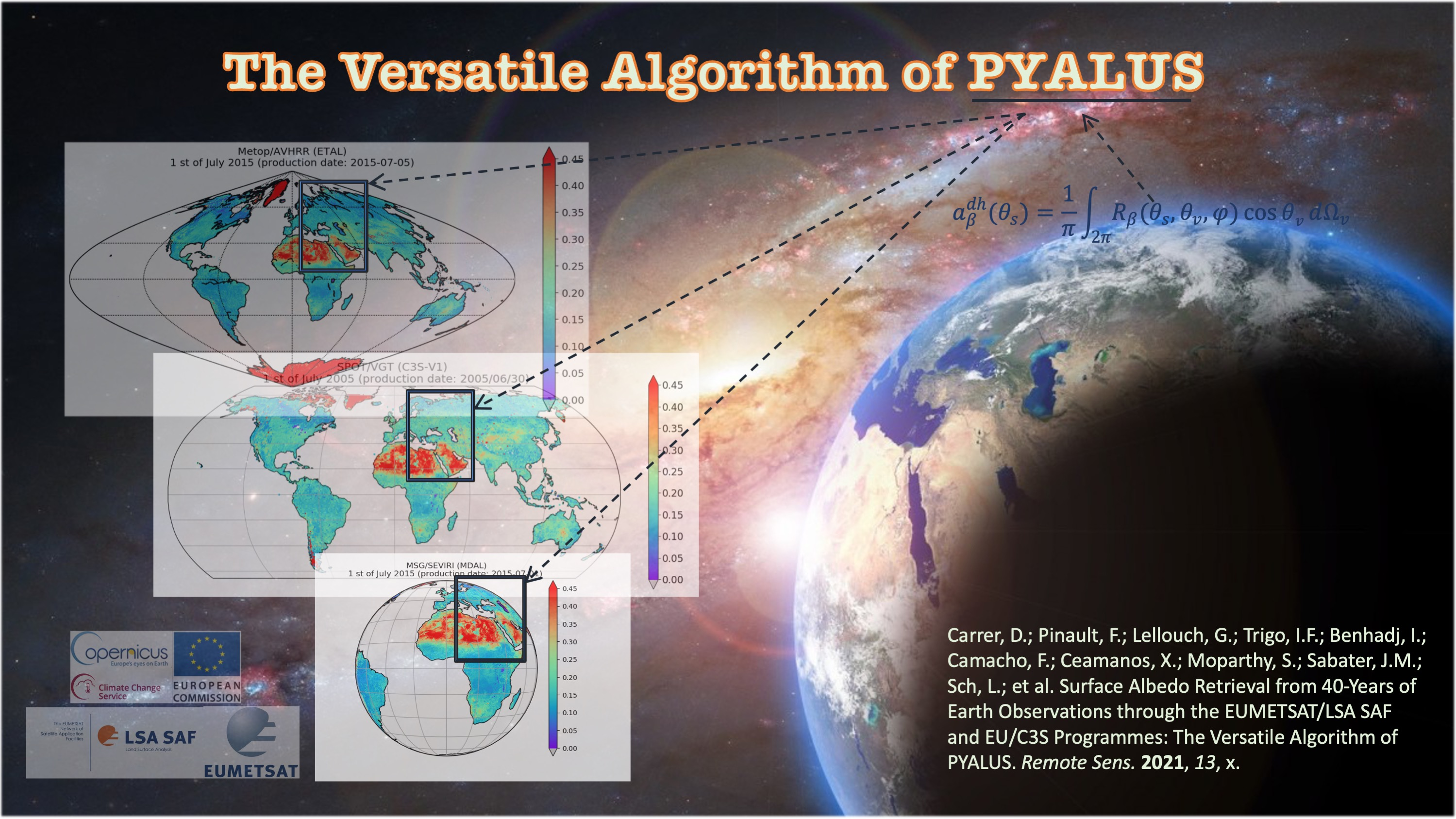
Surface Albedo Retrieval from 40-Years of Earth Observations through the EUMETSAT/LSA SAF and EU/C3S Programmes: The Versatile Algorithm of PYALUS


 ,
,  , ,
, , 
Abstract

1. Introduction
2. Algorithm Description
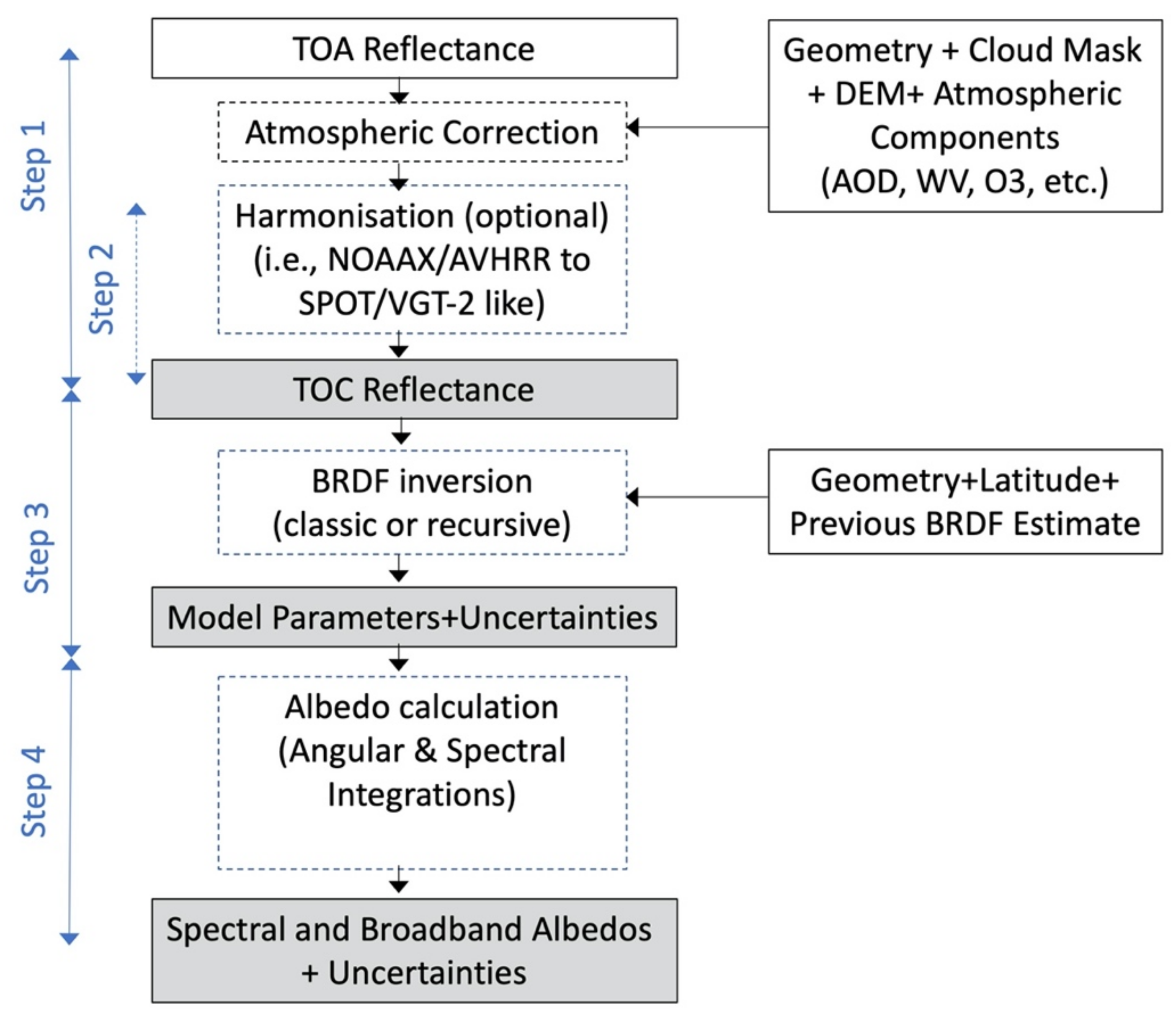
2.1. Method Overview
- Step 1.
- Atmospheric Correction: In a first step, the reflectances measured by the sensor at the Top of the Atmosphere (TOA) are used to estimate the reflectances at the Top of the Canopy (TOC) by applying the Simplified Method for the Atmospheric Correction (called SMAC) [36] of satellite measurements in the solar spectrum. This atmospheric correction process is described in Section 2.2.
- Step 2.
- Harmonisation (optional): This second step aims to harmonise data that are spectrally heterogeneous because they have been acquired by different sensors. The spectral harmonisation step is an optional step that allows the calculation of spectral albedos at fixed wavelengths (corresponding to a chosen reference sensor) from different sensors having different spectral characteristics (only used in C3S). First, a reference sensor is chosen (i.e., the four bands of SPOT/VGT2). The TOC reflectances from each given sensor are then harmonised into reflectances that would have been observed by the reference sensor on each of its bands. This method is further detailed in Section 2.3.
- Step 3.
- BRDF Inversion: In the third step, the measured TOC reflectances are used to fit the coefficients of a semi-empirical kernel-based reflectance model. These coefficients allow to rebuild the complete angular dependency of the bi-directional reflectance distribution function (BRDF). More information is presented in Section 2.4.
- Step 4.
- Albedo Computation: This step is composed of two main processes. First, the spectral albedo values, which are associated to the instrument channels, are determined by angular integration of the bi-directional reflectance factors. Second, the narrow-to-broadband conversion of albedos is performed. More information on this last step is given in Section 2.5.
2.2. Atmospheric Correction
- Gas content (mainly ozone and water vapour);
- Aerosol content and aerosol type;
- Molecular scattering mainly driven by the sea-level surface pressure and the surface elevation.
2.3. Spectral Harmonisation
2.4. BRDF Inversion
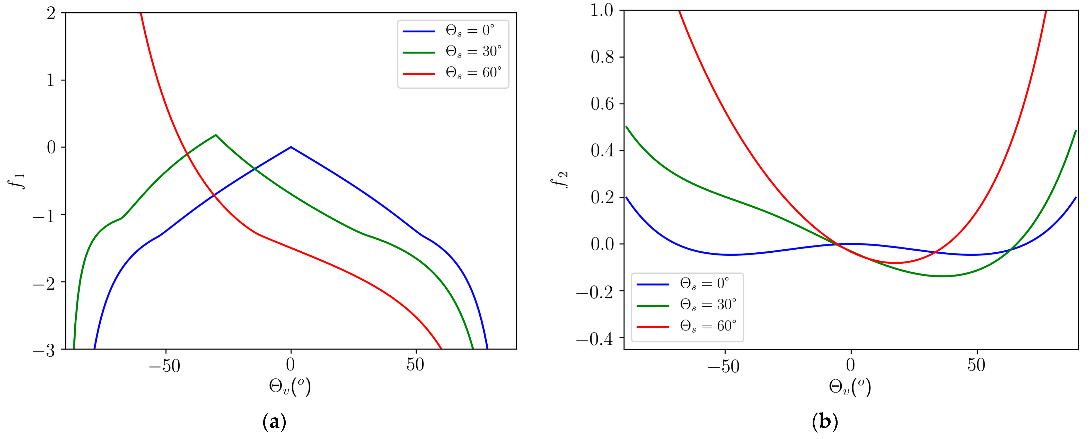
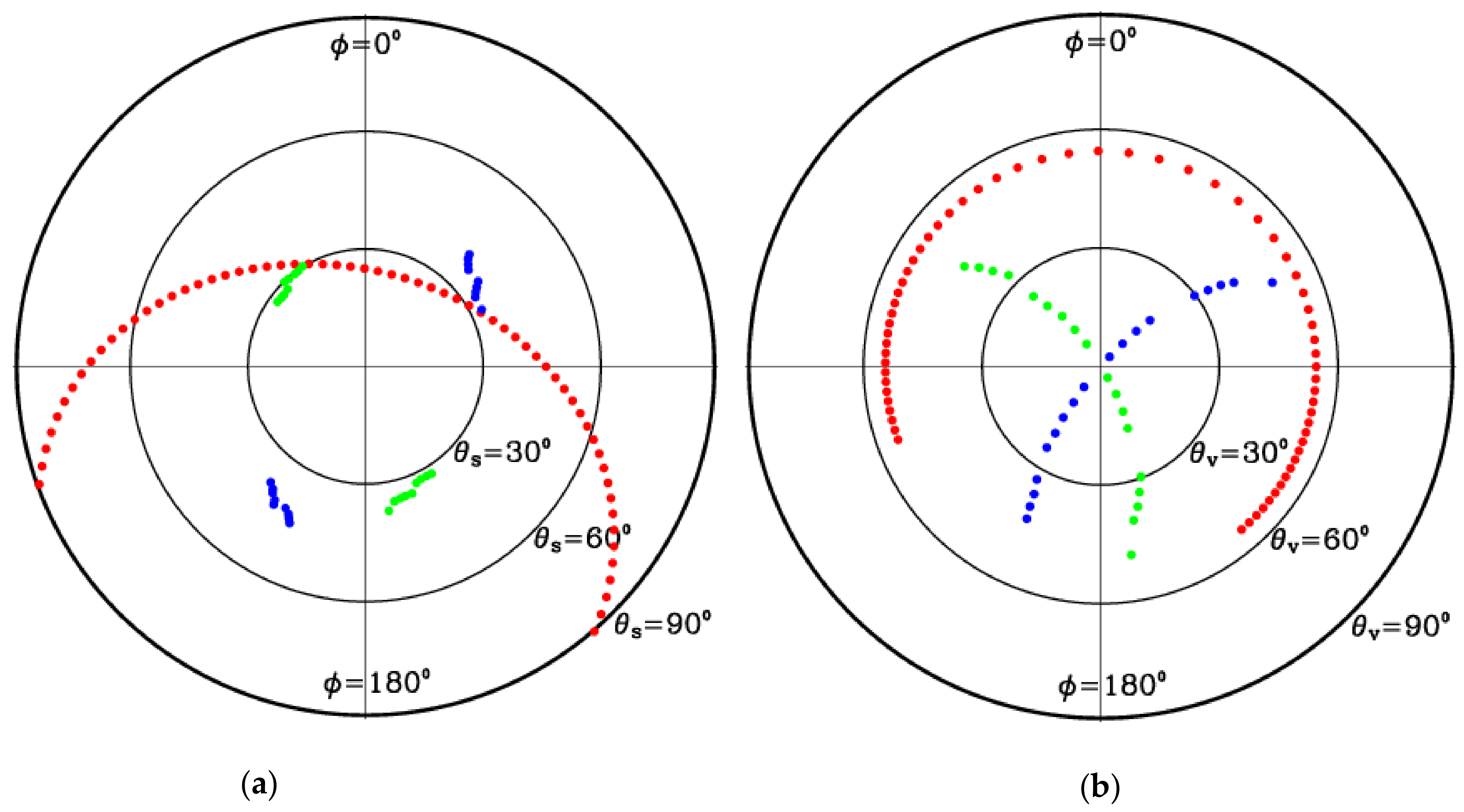
2.4.1. BRDF Models
2.4.2. Least Square Solution
2.4.3. Addition of a Priori Constraints Using a Recursive Method
2.4.4. Initialisation—Determination of the First a Priori Information
- Step 1—Spin up run—Run is performed for one year. The BRDF estimates of the last day of the spin up period is later used in Step 2 as first guess (a priori BRDF in Equation (7)). After one year, the KF has lost memory of its initial state: the lack of initial BRDF model has no more impact on the output product. In most cases, a shorter period (around 3 months) is sufficient to initialize the KF depending on the cloudiness, but one year has been chosen to take into account the vegetation cycle.
- Step 2—Actual run—Using the latest model from step 1, consider it as the initial a priori BRDF model and generate the product for the full period with Kalman filtering enabled.
2.4.5. Regularisation
k1 = k1reg ± σreg[k1]
k2 = k2reg ± σreg[k2]
2.5. Albedo Computation
2.5.1. Angular Integration
2.5.2. Narrow-to-Broadband Conversion
2.6. Extra-Filters—Impact of Clouds, Cloud Shadows, and Eclipses
3. Data
3.1. Input: Auxiliary Data
3.1.1. Digital Elevation Model (DEM)
3.1.2. Atmospheric Parameters
3.1.3. SMAC Coefficients
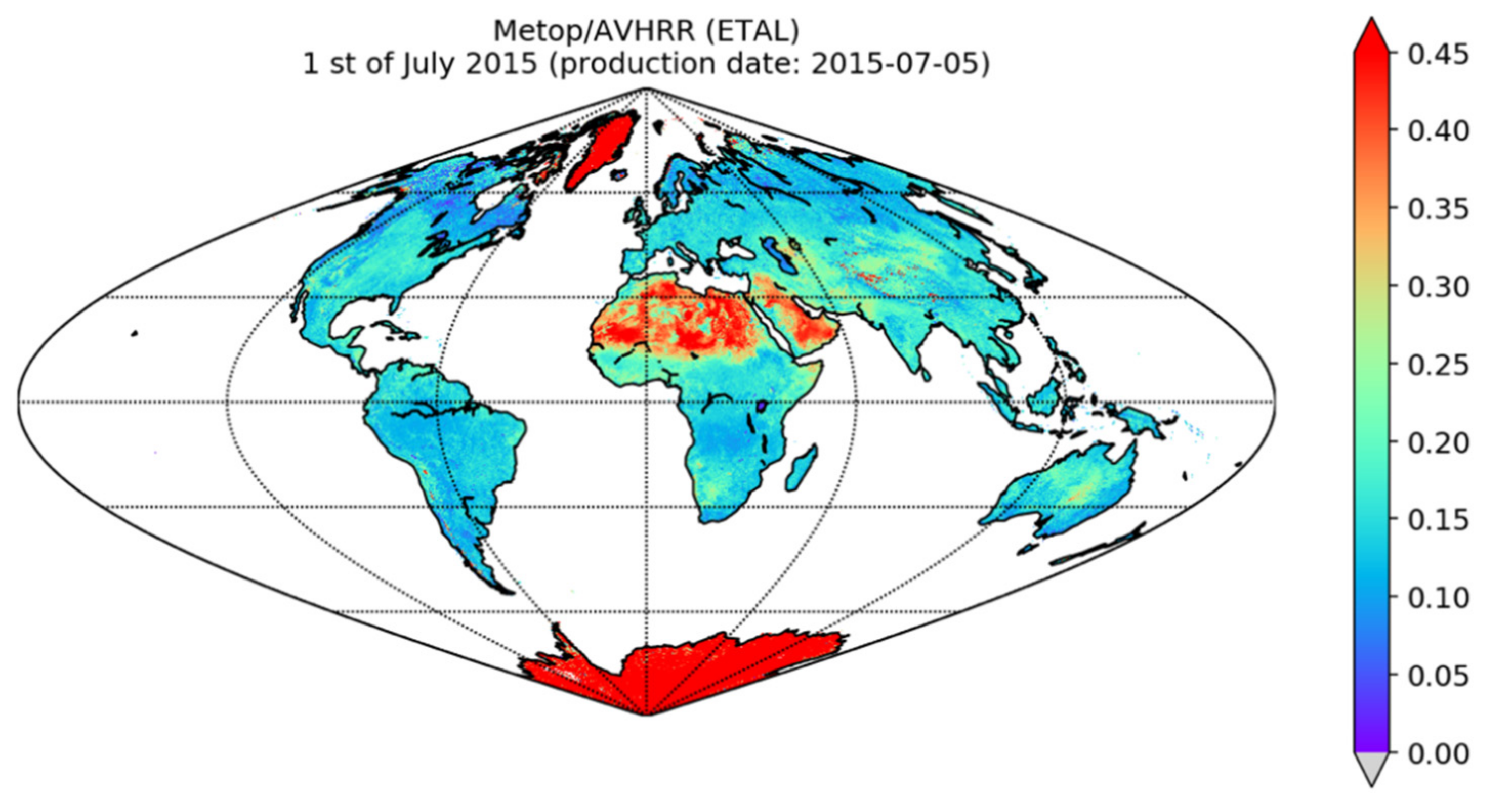
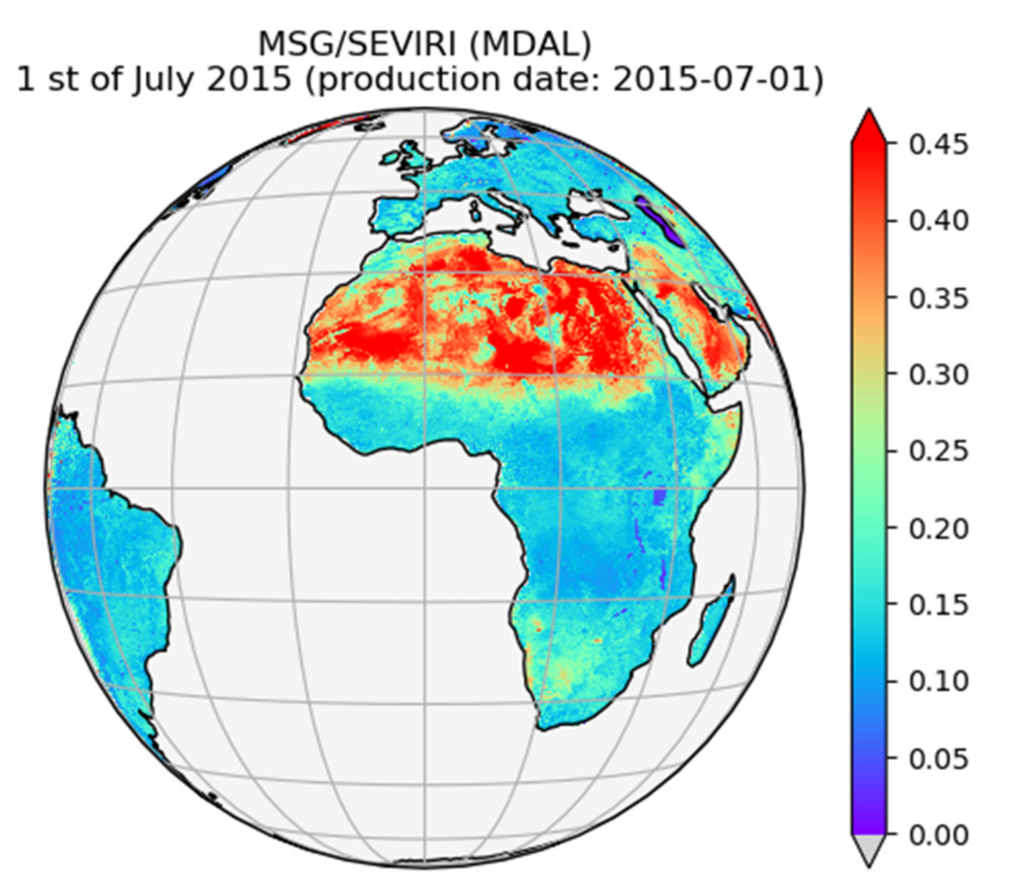
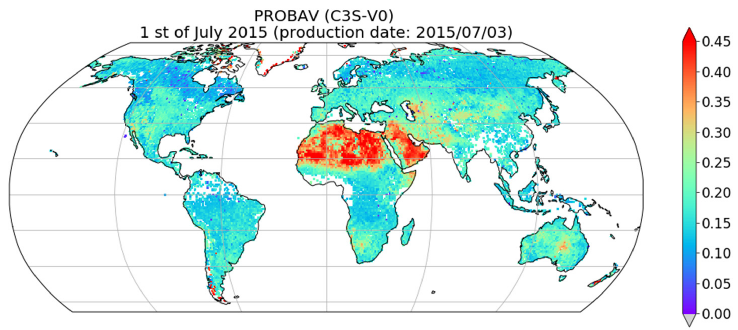
3.2. Radiance Inputs and Albedo Outputs
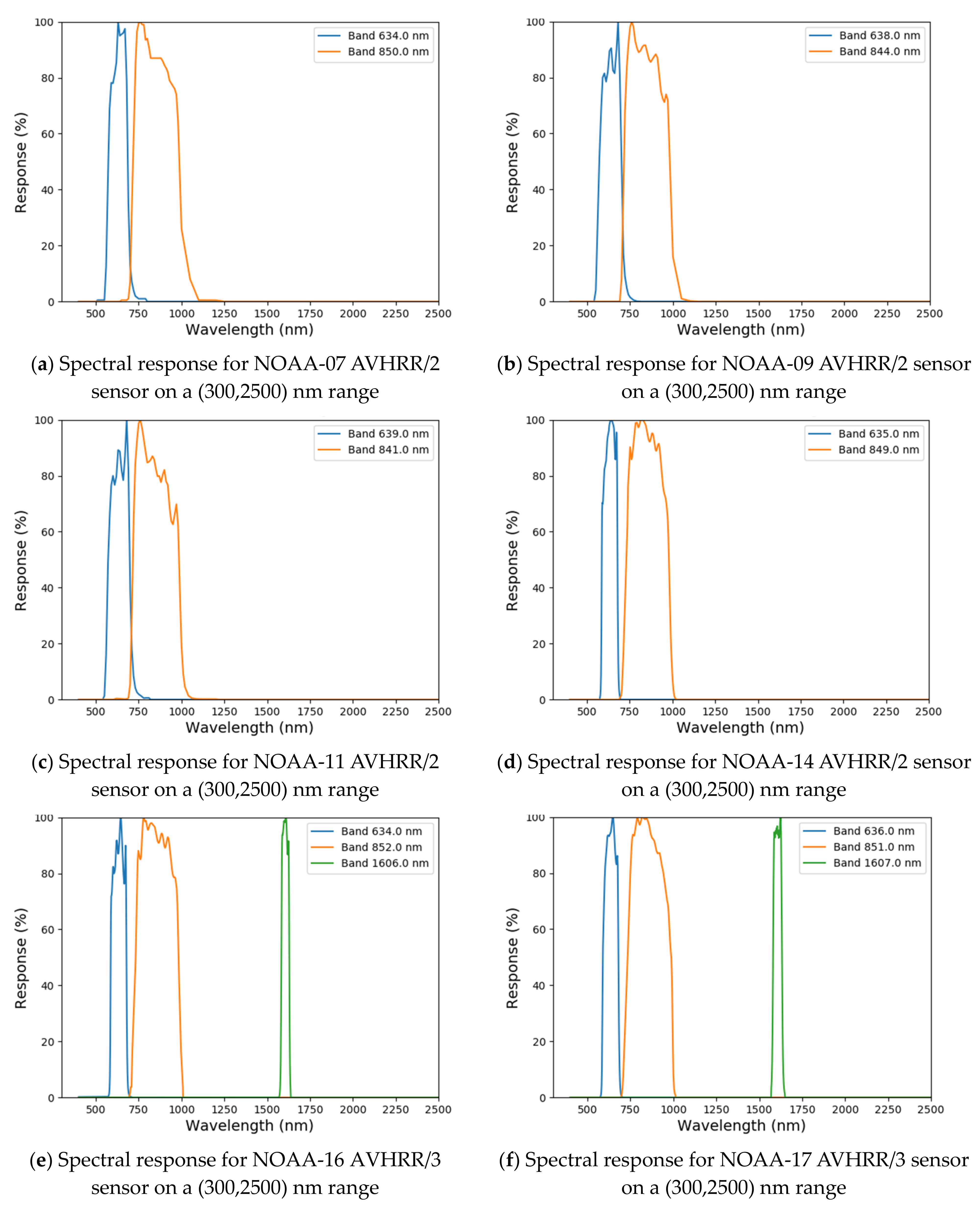
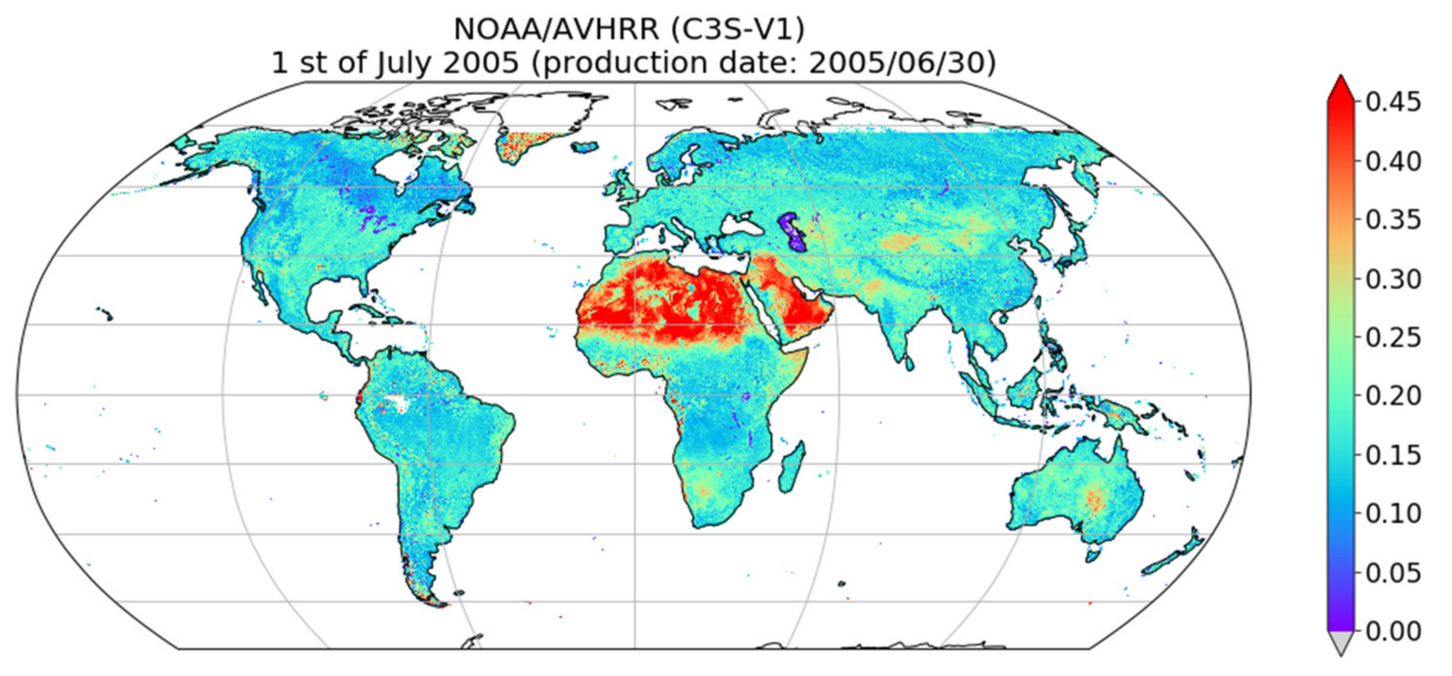
3.2.1. NOAA-X/AVHRR
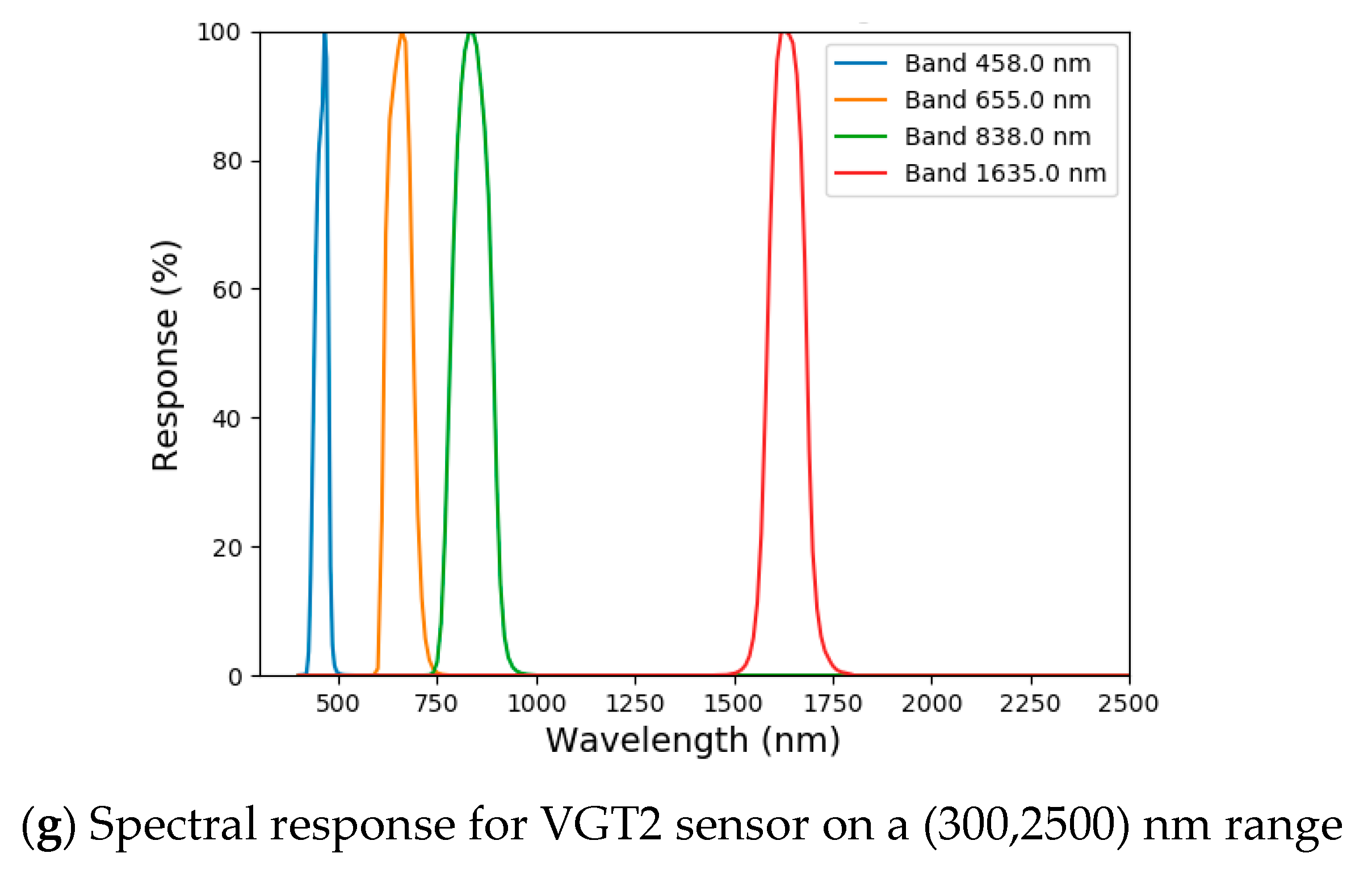
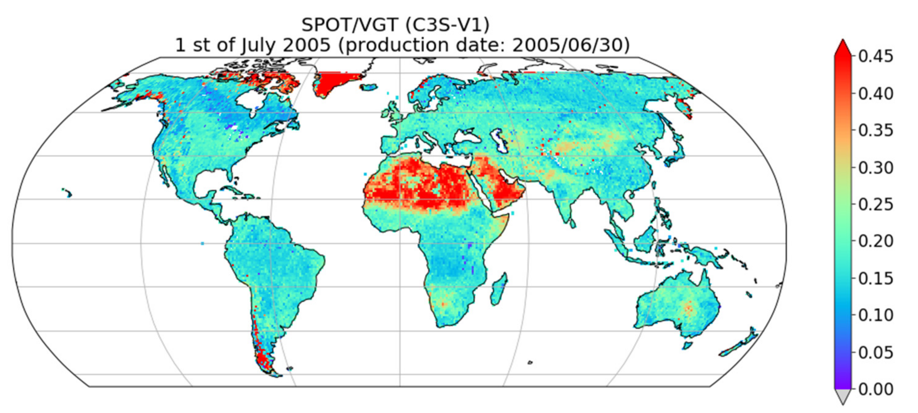
3.2.2. SPOT/VGT
3.2.3. Metop/AVHRR-3
3.2.4. MSG/SEVIRI
3.2.5. PROBA-V
4. Product Design
4.1. EUMETSAT and C3S Albedos
4.2. Albedo Characteristics: Spectral and Temporal
- Bi-hemispherical (‘white-sky’ or ‘WSA’) albedo products that are representative of diffuse conditions of illumination (typically cloudy sky conditions).
- Directional-hemispherical (‘black-sky’ or ‘BSA’) albedo products that are representative of direct conditions of illumination (typically clear sky conditions with pure atmosphere). As the surface is usually non-Lambertian and has directional properties, the value of surface albedo is given at a reference angle (solar position at the local noon).
- Spectral albedo for VGT-2 channels (B0, B2, B3 and MIR; Table 2);
- Broadband albedo for the visible (VIS) (0.4–0.7 µm), near-infrared (NIR) (0.7–4 µm) and the total shortwave (BB) (0.3–4 µm) spectral domains.
4.3. Product Content
5. Discussion and Known Issues
5.1. Differences between the LSA SAF and C3S Albedo Products
5.1.1. Atmospheric Correction
5.1.2. Spectral Harmonisation
5.2. Known Issues and Limitations
5.2.1. Residual of Clouds and Subpixel Clouds
5.2.2. Treatment of Snow Target Pixels
5.2.3. Calibration, Radiometry, and Orbit Drift
5.2.4. Atmospheric Correction
5.2.5. Review Process
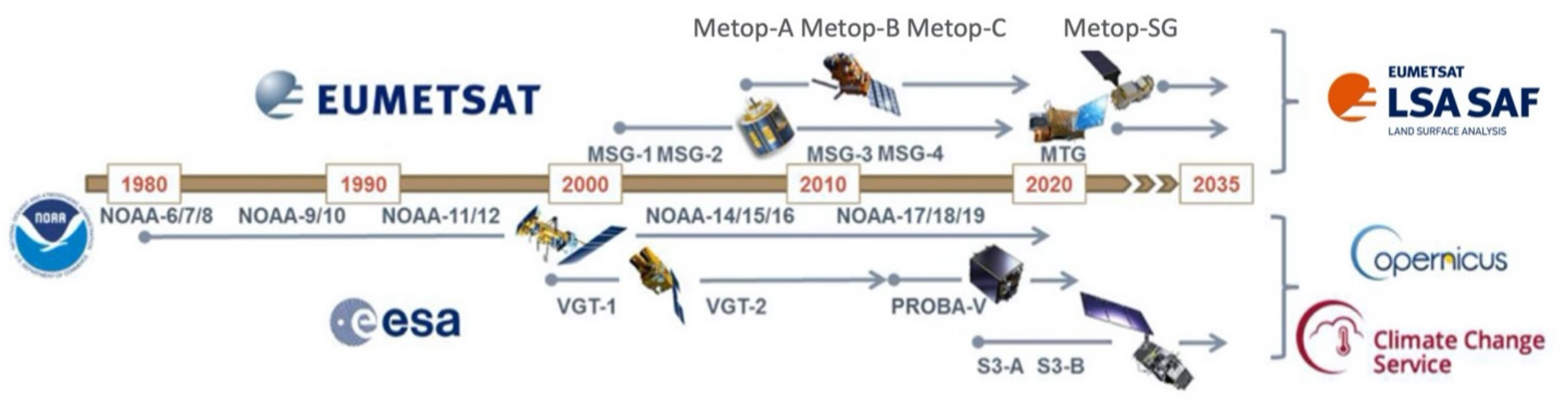
6. Roadmap for Product Continuity
7. Access to the Code Sources and Data Policy
8. Conclusions
Author Contributions
Funding
Institutional Review Board Statement
Informed Consent Statement
Data Availability Statement
Acknowledgments
Conflicts of Interest
Appendix A. Spectral Harmonisation

- The Fraction of Vegetation Cover (FCover) corresponds to the fraction of ground covered by green vegetation. It is a dimensionless parameter that takes values between 0 and 1.
- The Leaf Area Index (LAI) is another dimensionless quantity (m2/m2) that characterises plant canopies. It corresponds to the one-sided green leaf area per unit ground surface area.

| Name | Characteristics |
|---|---|
| Fcover | Uniform distribution on (0,1) |
| LAI | Normal distribution with mean = 4 × Fcover and standard deviation = 2, bounded within (0,10) |
| Hotspot parameter | Randomized on a uniform distribution between 0 and (1 + LAI/8)/2 |
| β′(NOAA-7/AVHRR) β(VGT2) | Sigma | ||||
| B0 | −0.0523 | 0.5813 | 0.0960 | 0.0309 | |
| B2 | 0.0097 | 1.0150 | −0.0203 | 0.0146 | |
| B3 | 0.0053 | −0.0746 | 1.0608 | 0.0162 | |
| MIR | 0.0216 | 0.5062 | 0.0873 | 0.0639 | |
| β′(NOAA-9/AVHRR) β(VGT2) | = RED | = NIR | = MIR | Sigma | |
| B0 | −0.0528 | 0.5820 | 0.0938 | 0.0311 | |
| B2 | 0.0088 | 1.0192 | −0.0258 | 0.0147 | |
| B3 | 0.0066 | −0.0802 | 1.0640 | 0.0162 | |
| MIR | 0.2016 | 0.5101 | 0.0829 | 0.0638 | |
| β′(NOAA-11/AVHRR) β(VGT2) | = RED | = NIR | = MIR | Sigma | |
| B0 | −0.0530 | 0.5807 | 0.0941 | 0.0312 | |
| B2 | 0.0084 | 1.0181 | −0.0256 | 0.0146 | |
| B3 | 0.0071 | −0.0802 | 1.0636 | 0.0162 | |
| MIR | 0.2015 | 0.5103 | 0.0825 | 0.0638 | |
| β′(NOAA-14/AVHRR) β(VGT2) | = RED | = NIR | = MIR | Sigma | |
| B0 | −0.0533 | 0.5706 | 0.1037 | 0.0312 | |
| B2 | 0.0082 | 0.9953 | −0.0036 | 0.0141 | |
| B3 | 0.0068 | −0.0382 | 1.0236 | 0.0155 | |
| MIR | 0.2020 | 0.5036 | 0.0880 | 0.0638 | |
| β′(NOAA-16/AVHRR) β(VGT2) | = RED | = NIR | = MIR | Sigma | |
| B0 | −0.0080 | 0.6869 | 0.1190 | −0.2241 | 0.0274 |
| B2 | −0.0010 | 0.9766 | −0.0068 | 0.0441 | 0.0135 |
| B3 | 0.0072 | −0.0287 | 1.0306 | −0.0160 | 0.0155 |
| MIR | 0.0119 | 0.0413 | 0.0210 | 0.9326 | 0.0141 |
| β′(NOAA-17/AVHRR) β(VGT2) | = RED | = NIR | = MIR | Sigma | |
| B0 | −0.0346 | 0.6920 | 0.1961 | −0.2742 | 0.0304 |
| B2 | −0.0032 | 0.9317 | −0.0476 | 0.1430 | 0.0132 |
| B3 | −0.0015 | −0.0749 | 1.0085 | 0.0793 | 0.0155 |
| MIR | 0.0710 | −0.2946 | −0.5074 | 1.8174 | 0.0346 |
References
- Carrer, D.; Meurey, C.; Ceamanos, X.; Roujean, J.L.; Calvet, J.C.; Liu, S. Dynamic mapping of snow-free vegetation and bare soil albedos at global 1km scale from 10-year analysis of MODIS satellite products. Remote Sens. Environ. 2014, 140, 420–432. [Google Scholar] [CrossRef]
- Davin, E.L.; de Noblet-Ducoudré, N. Climatic impact of global-scale deforestation: Radiative versus nonradiative processes. J. Clim. 2010, 23, 97–112. [Google Scholar] [CrossRef]
- Pielke, R.A.; Avissar, R. Influence of landscape structure on local and regional climate. Landsc. Ecol. 1990, 4, 133–155. [Google Scholar] [CrossRef]
- Ross, J. Role of phytometric investigations in the studies of plant stand architecture and radiation regime. In The Radiation Regime and Architecture of Plant Stands; Dr W. Junk Publishers: The Hague, The Netherlands, 1981; pp. 9–11. [Google Scholar]
- Cedilnik, J.; Carrer, D.; Mahfouf, J.F.; Roujean, J.L. Impact assessment of daily satellite-derived surface albedo in a limited-area NWP model. J. Appl. Meteorol. Climatol. 2012, 51, 1835–1854. [Google Scholar] [CrossRef]
- Carrer, D.; Lafont, S.; Roujean, J.-L.; Calvet, J.-C.; Meurey, C.; Le Moigne, P.; Trigo, I.F. Incoming Solar and Infrared Radiation Derived from METEOSAT: Impact on the Modeled Land Water and Energy Budget over France. J. Hydrometeorol. 2012, 13, 504–520. [Google Scholar] [CrossRef]
- Schaepman-Strub, G.; Schaepman, M.E.; Painter, T.H.; Dangel, S.; Martonchik, J.V. Reflectance quantities in optical remote sensing—Definitions and case studies. Remote Sens. Environ. 2006, 103, 27–42. [Google Scholar] [CrossRef]
- Bojinski, S.; Verstraete, M.; Peterson, T.C.; Richter, C.; Simmons, A.; Zemp, M. The Concept of Essential Climate Variables in Support of Climate Research, Applications, and Policy. Bull. Am. Meteorol. Soc. 2014, 95, 1431–1443. [Google Scholar] [CrossRef]
- Leroy, M.; Deuzé, J.L.; Bréon, F.M.; Hautecoeur, O.; Herman, M.; Buriez, J.C.; Tanré, D.; Bouffiès, S.; Chazette, P.; Roujean, J.-L. Retrieval of atmospheric properties and surface bidirectional reflectances over the land from POLDER/ADEOS. J. Geophys. Res. 1997, 102, 17023–17037. [Google Scholar] [CrossRef]
- Justice, C.O.; Vermote, E.; Townshend, J.R.; Defries, R.; Roy, D.P.; Hall, D.K.; Salomonson, V.V.; Privette, J.L.; Riggs, G.; Strahler, A.; et al. The moderate resolution imaging spectroradiometer (MODIS): Land remote sensing for global change research. IEEE Trans. Geosci. Remote Sens. 1998, 36, 1228–1249. [Google Scholar] [CrossRef]
- Wanner, W.; Strahler, A.H.; Hu, B.; Lewis, P.; Muller, J.P.; Li, X.; Schaaf, C.B.; Barnsley, M.J. Global retrieval of BRDF and albedo over land from EOS MODIS and MISR data: Theory and algorithm. J. Geophys. Res. 1997, 102, 17143–17161. [Google Scholar] [CrossRef]
- Strahler, A.H.; Muller, J.P. MODIS Science Team Members. MODIS BRDF/Albedo Product: Algorithm Theoretical Basis Document, Version 5.0. 1999. Available online: https://modis.gsfc.nasa.gov/data/atbd/atbd_mod09.pdf (accessed on 21 January 2021).
- Wang, Z.; Schaaf, C.B.; Chopping, M.J.; Strahler, A.H.; Wang, J.; Roman, M.O.; Rocha, A.V.; Woodcock, C.E.; Shuai, Y. Evaluation of Moderate-resolution Imaging Spectroradiometer (MODIS) snow albedo product (MCD43A) over tundra. Remote Sens. Environ. 2012, 117, 264–280. [Google Scholar] [CrossRef]
- Schaaf, C.B.; Gao, F.; Strahler, A.H.; Lucht, W.; Li, X.; Tsang, T.; Strugnell, N.C.; Zhang, X.; Jin, Y.; Muller, J.-P.; et al. First Operational BRDF, Albedo and Nadir Reflectance Products from MODIS. Remote Sens. Environ. 2002, 83, 135–148. [Google Scholar] [CrossRef]
- Wang, Z.; Schaaf, C.B.; Sun, Q.; Shuai, Y.; Román, M.O. Capturing rapid land surface dynamics with Collection V006 MODIS BRDF/NBAR/Albedo (MCD43) products. Remote Sens. Environ. 2018, 207, 50–64. [Google Scholar] [CrossRef]
- Diner, D.J.; Beckert, J.C.; Reilly, T.H.; Bruegge, C.J.; Conel, J.E.; Kahn, R.A.; Martonchik, J.V.; Ackerman, T.P.; Davies, R.; Gerstl, S.A.; et al. Multi-angle imaging spectro-radiometer (MISR) in- strument description and experiment overview. IEEE Trans. Geosci. Remote Sens. 1998, 36, 1072–1087. [Google Scholar] [CrossRef]
- Pinty, B.; Roveda, F.; Verstraete, M.M.; Gobron, N.; Govaerts, Y.; Martonchik, J.V.; Diner, D.J.; Kahn, R.A. Surface albedo retrieval from Meteosat. J. Geophys. Res. 2000, 105, 18099–18134. [Google Scholar] [CrossRef]
- Pinty, B.; Lattanzio, A.; Martonchik, J.V.; Verstraete, M.M.; Gobron, N.; Taberner, M.; Widlowski, J.L.; Dickinson, R.E.; Govaerts, Y. Coupling diffuse sky radiation and surface Albedo. J. Atmos. Sci. 2005, 62, 2580–2591. [Google Scholar] [CrossRef]
- Muller, J.P.; López, G.; Watson, G.; Shane, N.; Kennedy, T.; Yuen, P.; Lewis, P.; Fischer, J.; Guanter, L.; Domench, C.; et al. The ESA GlobAlbedo project for mapping the Earth’s land surface albedo for 15 years from European sensors. In Proceedings of the IEEE Geoscience and Remote Sensing Symposium (IGARSS), Munich, Germany, 22–27 July 2012. [Google Scholar]
- Muller, J.P. GlobAlbedo Final Validation Report; University College London: London, UK, 2013; Available online: http://www.globalbedo.org/docs/GlobAlbedo_FVR_V1_2_web.pdf (accessed on 10 June 2020).
- Liang, S.; Zhao, X.; Liu, S.; Yuan, W.; Cheng, X.; Xiao, Z.; Zhang, X.; Liu, Q.; Cheng, J.; Tang, H.; et al. A long-term Global LAnd Surface Satellite (GLASS) data-set for environmental studies. Int. J. Digit. Earth 2013, 6, 5–33. [Google Scholar] [CrossRef]
- Govaerts, Y.M.; Wagner, S.; Lattanzio, A.; Watts, P. Joint retrieval of surface reflectance and aerosol optical depth from MSG/SEVIRI observations with an optimal estima- tion approach: 1. Theory. J. Geophys. Res. 2010, 115, D02203. [Google Scholar] [CrossRef]
- Carrer, D.; Roujean, J.L.; Hautecoeur, O.; Elias, T. Daily estimates of aerosol optical thickness over land surface based on a directional and temporal analysis of SEVIRI MSG visible observations. J. Geophys. Res. 2010, 115, D10. [Google Scholar] [CrossRef]
- Barnsley, M.J.; Strahler, A.H.; Morris, K.P.; Muller, J.P. Sampling the surface bidirectional reflectance distribution function (BRDF): Evaluation of current and future satellite sensors. Remote Sens. Rev. 1994, 8, 271–311. [Google Scholar] [CrossRef]
- Strahler, A.H. Vegetation canopy reflectance modeling—Recent developments and remote sensing perspectives. Remote Sens. Rev. 1997, 15, 179–194. [Google Scholar] [CrossRef]
- Hu, B.; Lucht, W.; Li, X.; Strahler, A.H. Validation of kernel-driven models for global modeling of bidirectional reflectance. Remote Sens. Environ. 1997, 62, 201–214. [Google Scholar] [CrossRef]
- Wanner, W.; Li, X.; Strahler, A.H. On the derivation of kernels for kernel-driven models of bidirectional reflectance. J. Geophys. Res. Atmos. 1995, 100, 21077–21089. [Google Scholar] [CrossRef]
- Lucht, W.; Schaaf, C.B.; Strahler, A.H. An algorithm for the retrieval of albedo from space using semiempirical BRDF models. IEEE Trans. Geosci. Remote Sens. 2000, 38, 977–998. [Google Scholar] [CrossRef]
- Geiger, B.; Carrer, D.; Franchisteguy, L.; Roujean, J.L.; Meurey, C. Land Surface Albedo derived on a daily basis from Meteosat Second Generation Observations. IEEE Trans. Geosci. Remote Sens. 2008, 46, 3841–3856. [Google Scholar] [CrossRef]
- Carrer, D.; Moparthy, S.; Lellouch, G.; Ceamanos, X.; Pinault, F.; Freitas, S.C.; Trigo, I.F. Land Surface Albedo Derived on a Ten Daily Basis from Meteosat Second Generation Observations: The NRT and Climate Data Record Collections from the EUMETSAT LSA SAF. Remote Sens. 2018, 10, 1262. [Google Scholar] [CrossRef]
- Wang, D.D.; Liang, S.L.; He, T.; Yu, Y.Y. Direct Estimation of Land Surface Albedo from VIIRS Data: Algorithm Improvement and Preliminary Validation. J. Geophys. Res. Atmos. 2013, 118, 12577–12586. [Google Scholar] [CrossRef]
- Wang, D.D.; Liang, S.L.; Zhou, Y.; He, T.; Yu, Y.Y. A New Method for Retrieving Daily Land Surface Albedo from VIIRS Data. IEEE Trans. Geosci. Remote Sens. 2017, 55, 1765–1775. [Google Scholar] [CrossRef]
- Trigo, I.F.; Dacamara, C.C.; Viterbo, P.; Roujean, J.L.; Olesen, F.; Barroso, C.; Camacho-de-Coca, F.; Carrer, D.; Freitas, S.C.; García-Haro, J.; et al. The satellite application facility for land surface analysis. Int. J. Remote Sens. 2011, 32, 2725–2744. [Google Scholar] [CrossRef]
- Lellouch, G.; Carrer, D.; Vincent, C.; Pardé, M.C.; Frietas, S.; Trigo, I.F. Evaluation of Two Global Land Surface Albedo Datasets Distributed by the Copernicus Climate Change Service and the EUMETSAT LSA SAF. Remote Sens. 2020, 12, 1888. [Google Scholar] [CrossRef]
- Sanchez-Zapero, J.; Camacho, F.; Martinez-Sanchez, E.; Lacaze, R.; Carrer, D.; Pinault, F.; Benhadj, I.; Munoz-Sabater, J. Quality Assessment of PROBA-V Surface Albedo V1 for the Continuity of the Copernicus Climate Change Service. Remote Sens. 2020, 12, 2596. [Google Scholar] [CrossRef]
- Rahman, H.; Dedieu, G. SMAC: A simplified method for the atmospheric correction of satellite measurements in the solar spectrum. Intern. J. Remote Sens. 1994, 15, 123–143. [Google Scholar] [CrossRef]
- Vermote, E.F.; Tanré, D.; Deuze, J.L.; Herman, M.; Morcette, J.J. Second Simulation of the Satellite Signal in the Solar Spectrum, 6S: An Overview. IEEE Trans. Geosci. Remote Sens. 1997, 35, 675–686. [Google Scholar] [CrossRef]
- Press, W.H.; Teukolsky, S.A.; Vetterling, W.T.; Flannery, B.P. Numerical Recipes in Fortran; Cambridge University Press: Cambridge, UK, 1992. [Google Scholar]
- Li, X.; Gao, F.; Wang, J.; Strahler, A. A priori knowledge accumulation and its application to linear BRDF model inversion. J. Geophys. Res. 2001, 106, 11925–11935. [Google Scholar] [CrossRef]
- Hagolle, O.; Lobo, A.; Maisongrande, P.; Cabot, F.; Duchemin, B.; de Pereyra, A. Quality assessment and improvement of temporally composited products of remotely sensed imagery by combination of VEGETATION 1 & 2 images. Remote Sens. Environ. 2004, 94, 172–186. [Google Scholar]
- Carrer, D.; Roujean, J.L.; Meurey, C. Comparing operational MSG/SEVIRI land surface albedo products from Land SAF with ground measurements and MODIS. IEEE Trans. Geosci. Remote Sens. 2010, 48, 1714–1728. [Google Scholar] [CrossRef]
- Pokrovsky, I.O.; Pokrovsky, O.M.; Roujean, J.-L. Development of an operational procedure to estimate surface albedo from the SEVIRI/MSG observing system in using POLDER BRDF measurements. Remote Sens. Environ. 2003, 87, 198–242. [Google Scholar] [CrossRef]
- Hook, S.J. ASTER Spectral Library. 1998. Available online: http://speclib.jpl.nasa.gov (accessed on 10 June 2020).
- Verhoef, W. Light scattering by leaf layers with application to canopy reflectance modeling, the SAIL model. Remote Sens. Environ. 1984, 16, 125–141. [Google Scholar] [CrossRef]
- Toté, C.; Swinnen, E.; Sterckx, S.; Clarijs, D.; Quang, C.; Maes, R. Evaluation of the SPOT/VEGETATION Collection 3 reprocessed dataset: Surface reflectances and NDVI. Remote Sens. Environ. 2017, 201, 219–233. [Google Scholar] [CrossRef]
- Sterckx, S.; Benhadj, I.; Duhoux, G.; Livens, S.; Dierckx, W.; Goor, E.; Adriaensen, S.; Heyns, W.; Van Hoof, K.; Strackx, G.; et al. The PROBA-V mission: Image processing and calibration. Int. J. Remote Sens. 2014, 35, 2565–2588. [Google Scholar] [CrossRef]
- Schmetz, J.; Pili, P.; Tjemkes, S.; Just, D.; Kerkmann, J.; Rota, S.; Ratier, A. An introduction to Meteosat Second Generation (MSG). Bull. Am. Meteor. Soc. 2002, 83, 977–992. [Google Scholar] [CrossRef]
- Carrer, D.; Smets, B.; Ceamanos, X.; Roujean, W.H.J.-L.; Lacaze, R. Copernicus Global Land SPOT/VEGETATION and PROBA-V Surface Albedo Products—1 Km Version 1; Algorithm Theoretical Basis Document, Issue 2.11, Copernicus Global Land Operations Vegetation and Energy CGLOPS-1. Framework Service Contract N° 199494; Join Research Center (JRC): Ispra, Italy, 2018. [Google Scholar]
- Geiger, B.; Samain, O. Albedo Determination, Algorithm Theoretical Basis Document, of the CYCLOPES Project; Version 2.0.; Météo-France/CNRM: Paris, France, 2004; p. 25. [Google Scholar]
- Grenfell, T.C.; Perovich, D.K. Seasonal and spatial evolution of albedo in a snow ice land ocean environment. J. Geophys. Res. 2004, 109, C01001. [Google Scholar] [CrossRef]
- Planque, C.; Carrer, D.; Roujean, J.-L. Analysis of MODIS albedo changes over steady woody covers in France during the period of 2001–2013. Remote Sens. Environ. 2017, 191, 13–29. [Google Scholar] [CrossRef]
- Lebourgeois, F.; Pierrat, J.-C.; Perez, V.; Piedallu, C.; Cecchini, S.; Ulrich, E. Simulating phenological shifts in French temperate forests under two climatic change scenarios and four driving global circulation models. Int. J. Biometeorol. 2010, 54, 563–581. [Google Scholar] [CrossRef]
- Meirink, J.F.; Roebeling, R.A.; Stammes, P. Inter-calibration of polar imager solar channels using SEVIRI. Atmos. Meas. Tech. 2013, 6, 2495–2508. [Google Scholar] [CrossRef]
- Proud, S.R.; Fensholt, R.; Rasmussen, M.O.; Sandholt, I. A compar- ison of the effectiveness of 6S and SMAC in correcting for atmospheric interference of Meteosat Second Generation images. J. Geophys. Res. 2010, 115, D17209. [Google Scholar] [CrossRef]
- Wang, Z.; Schaaf, C.; Lattanzio, A.; Carrer, D.; Grant, I.; Román, M.; Camacho, F.; Yu, Y.; Sánchez-Zapero, J.; Nickeson, J. Best Practice for Satellite Derived Land Product Validation. In Global Surface Albedo Product Validation Best Practices Protocol; Version, 1.0; Wang, Z., Nickeson, J., Román, M., Eds.; Land Product Validation Subgroup (WGCV/CEOS): Washington, DC, USA, 2019; p. 45. [Google Scholar] [CrossRef]
- Samain, O.; Geiger, B.; Roujean, J.L. Spectral Normalization and Fusion of Optical Sensors for the Retrieval of BRDF and Albedo: Application to VEGETATION, MODIS, and MERIS Data Sets. IEEE Trans. Geosci. Remote Sens. 2006, 44, 3166–3179. [Google Scholar] [CrossRef]
- Jacquemoud, S.; Baret, F. PROSPECT: A model of leaf optical properties spectra. Remote Sens. Environ. 1990, 34, 75–91. [Google Scholar] [CrossRef]
- Kuusk, A. Determination of vegetation canopy parameters from optical measurements. Remote Sens. Environ. 1991, 37, 207–218. [Google Scholar] [CrossRef]
- Jacquemoud, S.; Verhoef, W.; Baret, F.; Bacour, C.; Zarco-Tejada, P.J.; Asner, G.P.; François, C.; Ustin, S.L. PROSPECT+SAIL models: A review of use for vegetation characterization. Remote Sens. Environ. 2009, 113, 56–66. [Google Scholar] [CrossRef]
- Zou, H.; Hastie, T. Regularisation and Variable Selection via the Elastic Net. J. R. Stat. Soc. Ser. B 2004, 67, 301–320. [Google Scholar] [CrossRef]


| Product | Sensor (Coverage) | Product ID (Type) | Production Frequency | Composite Window | Temporal Characteristic Time Scale | Spatial Scale | Composition Method | BRDF Model | Atmospheric Correction | Documentation and Data Link Accesses | Temporal Coverage | Product Continuity |
|---|---|---|---|---|---|---|---|---|---|---|---|---|
| Albedo (CDR) | NOAA-X/AVHRR (global) | C3S-V1 | 10-day | 20-day | 10-day | 1–4 km | recursive | Li-Sparse Reciprocal | Hygeos | C3S-V1 access | 1981–2015 | C3S-V2 |
| Albedo (CDR) | SPOT/VGT (global) | C3S-V1 | 10-day | 20-day | 10-day | 1 km | recursive | Li-Sparse Reciprocal | Hygeos | C3S-V1 access | 1998–2014 | C3S-V2 |
| Albedo (ICDR) | PROBA-V (global) | C3S-V0 | 10-day | 30-day | 20-day | 1 km | recursive | Roujean | VITO | C3S-V0 access | 2014+ | C3S-V2 |
| Albedo (NRT) | SPOT/VGT (global) | VGP-P | 10-day | 30-day | 20-day | 1 km | recursive | Roujean | VITO | CGLS access | 1998–2014 | |
| Albedo (NRT) | PROBA-V (global) | PROBA-V L2A | 10-day | 30-day | 20-day | 1 km | recursive | Roujean | VITO | CGLS access | 2014–2020 | |
| Albedo (NRT) | MSG/SEVIRI (Africa, Europe, South America) | LSA-101 | 1-day | 1-day | 5-day | SEVIRI grid | recursive | Roujean | Météo France | LSA-101 access | 2005+ | LSA-107 (MTG/FCI) |
| Albedo (NRT) | MSG/SEVIRI (Africa, Europe, South America) | LSA-102 | 10-day | 30-day | 30-day | SEVIRI grid | classic | Roujean | Météo France | LSA-102 access | 2009+ | LSA-108 (MTG/FCI) |
| Albedo (CDR) | MSG/SEVIRI (Africa, Europe, South America) | LSA-150 | 10-day | 30-day | 30-day | SEVIRI grid | classic | Roujean | Météo France | LSA-150 access | 2005–2015 | |
| Albedo (NRT) | Metop/AVHRR (global) | LSA-103 | 10-day | 20-day | 10-day | 1 km | recursive | Li-Sparse Reciprocal | Météo France | LSA-103 access | 2015+ | LSA-110, 111 (Metop-SG/METimage, 3MI) |
| Band | VGT-2 (µm) |
|---|---|
| Blue (B0) | 0.439–0.476 (0.458) |
| Red (B2) | 0.616–0.690 (0.653) |
| NIR (B3) | 0.783–0.892 (0.838) |
| SWIR (MIR) | 1.584–1.685 (1.635) |
| Band | SEVIRI (µm) | AVHRR-3 (µm) |
|---|---|---|
| Blue (B0) | - | 0.439–0.476 (0.458) |
| Red (B2) | 0.56–0.71 (0.635) | 0.616–0.690 (0.653) |
| NIR (B3) | 0.74–0.88 (0.81) | 0.783–0.892 (0.838) |
| SWIR (MIR) | 1.50–1.78 (1.64) | 1.584–1.685 (1.635) |
Publisher’s Note: MDPI stays neutral with regard to jurisdictional claims in published maps and institutional affiliations. |
© 2021 by the authors. Licensee MDPI, Basel, Switzerland. This article is an open access article distributed under the terms and conditions of the Creative Commons Attribution (CC BY) license (http://creativecommons.org/licenses/by/4.0/).
Share and Cite
Carrer, D.; Pinault, F.; Lellouch, G.; Trigo, I.F.; Benhadj, I.; Camacho, F.; Ceamanos, X.; Moparthy, S.; Munoz-Sabater, J.; Schüller, L.; et al. Surface Albedo Retrieval from 40-Years of Earth Observations through the EUMETSAT/LSA SAF and EU/C3S Programmes: The Versatile Algorithm of PYALUS. Remote Sens. 2021, 13, 372. https://doi.org/10.3390/rs13030372
Carrer D, Pinault F, Lellouch G, Trigo IF, Benhadj I, Camacho F, Ceamanos X, Moparthy S, Munoz-Sabater J, Schüller L, et al. Surface Albedo Retrieval from 40-Years of Earth Observations through the EUMETSAT/LSA SAF and EU/C3S Programmes: The Versatile Algorithm of PYALUS. Remote Sensing. 2021; 13(3):372. https://doi.org/10.3390/rs13030372
Chicago/Turabian StyleCarrer, Dominique, Florian Pinault, Gabriel Lellouch, Isabel F. Trigo, Iskander Benhadj, Fernando Camacho, Xavier Ceamanos, Suman Moparthy, Joaquin Munoz-Sabater, Lothar Schüller, and et al. 2021. "Surface Albedo Retrieval from 40-Years of Earth Observations through the EUMETSAT/LSA SAF and EU/C3S Programmes: The Versatile Algorithm of PYALUS" Remote Sensing 13, no. 3: 372. https://doi.org/10.3390/rs13030372
APA StyleCarrer, D., Pinault, F., Lellouch, G., Trigo, I. F., Benhadj, I., Camacho, F., Ceamanos, X., Moparthy, S., Munoz-Sabater, J., Schüller, L., & Sánchez-Zapero, J. (2021). Surface Albedo Retrieval from 40-Years of Earth Observations through the EUMETSAT/LSA SAF and EU/C3S Programmes: The Versatile Algorithm of PYALUS. Remote Sensing, 13(3), 372. https://doi.org/10.3390/rs13030372