Comparison between Three Registration Methods in the Case of Non-Georeferenced Close Range of Multispectral Images

Abstract

Cucumber powdery mildew, which is caused by Podosphaera xanthii, is a major disease that has a significant economic impact in cucumber greenhouse production. It is necessary to develop a non-invasive fast detection system for that disease. Such a system will use multispectral imagery acquired at a close range with a camera attached to a mobile cart’s mechanic extension. This study evaluated three image registration methods applied to non-georeferenced multispectral images acquired at close range over greenhouse cucumber plants with a MicaSense^® RedEdge camera. The detection of matching points was performed using Speeded-Up Robust Features (SURF), and outliers matching points were removed using the M-estimator Sample Consensus (MSAC) algorithm. Three geometric transformations (affine, similarity, and projective) were considered in the registration process. For each transformation, we mapped the matching points of the blue, green, red, and NIR band images into the red-edge band space and computed the root mean square error (RMSE in pixel) to estimate the accuracy of each image registration. Our results achieved an RMSE of less than 1 pixel with the similarity and affine transformations and of less than 2 pixels with the projective transformation, whatever the band image. We determined that the best image registration method corresponded to the affine transformation because the RMSE is less than 1 pixel and the RMSEs have a Gaussian distribution for all of the bands, but the blue band.

1. Introduction

In Canada, there are close to 16.9 million m² greenhouses [1], about 25% (4.3 million m²) being dedicated to cucumber (Cucumis sativus L.) production [1], which led to a total cucumber production of 206,228 metric tons in 2017 [1]. However, even with many greenhouse crops, cucumber production might be subject to fungal diseases, which are a major limiting factor in the production system [2]. One of them is powdery mildew, which is caused by the fungus Podosphaera xanthii. This disease may lead to yield losses between 30 and 50% of the total production [3]. The pathogen is biotrophic, i.e., it interacts with the host without killing the host cells to obtain nutrients [4]. Powdery mildew grows haustorium that causes internal structural damage of colonized cell walls of leaves, petioles, and stems, establishing a close connection with the lying beneath the host cells [5,6]. Such changes in the cell walls should be better detected using near-infrared imagery [7]. With the development of the disease, the infected plants are subjected to chemical changes, inducing chlorophyll degradation, which can be detected in the visible region of the electromagnetic spectrum [8,9]. Acquiring imagery in the visible and near-infrared regions of the electromagnetic spectrum requires the use of multispectral cameras. Most of the studies that use multispectral cameras to detect crop diseases were performed using either airborne, satellite, or UAV imagery in field conditions [10,11]. For greenhouse conditions, studies on the detection of cucumber powdery mildew mainly used RGB images acquired over single leaves having visible symptoms [12,13,14,15]. RGB cameras have the advantage of being made of a single sensor that uses filters to produce the red, green, and blue image. As a result, the three images automatically well align. However, multispectral cameras are made of more than one sensor, and the distance between the sensors makes the images not aligned (Figure 1). Such an alignment is easy to perform when the images are georeferenced such as for airborne, satellite, or UAV imagery. However, in the case of imagery acquired with a robot in a greenhouse, the imagery is not georeferenced, and there is a need to develop an image registration method for properly aligning the band images. In this case, the images that need to be registered (known as the moving images) are registered as a function of a reference image (known as the fixed image) [16]. The registration process involves the detection of features through a feature detector algorithm and their location on the moving and fixed images to geometrically transform the moving image into the fixed image space [17,18]. The feature detector algorithm should be such that it has high repeatability, i.e., it needs to detect the same interest points or key points under different viewing conditions. The detector must also be robust to noise, detection errors, and geometric and photometric deformations [19,20]. Finally, it needs to have a short computation time as possible [21].

This study aims to evaluate three methods of image registration in the case of non-georeferenced multispectral images acquired at close range over greenhouse cucumber plants with a MicaSense^® RedEdge camera (MicaSense, Inc., Seattle, Washington, USA), which was attached to a mechanic extension of a mobile cart. The three methods use the blue, green, red, and NIR bands as moving images and the red-edge band as the fixed reference image because the related sensor has a central position on the camera (Figure 1). In the three methods, we detected and extracted features with the Speeded-Up Robust Features (SURF) algorithm, which is a scale and rotation invariant detector and descriptor developed by Bay et al. [19]. The main advantages of the SURF algorithm over other well-known detectors such as the Scale-Invariant Feature Transform (SIFT) [22] is its lower computational cost and faster performance [19,20,21,23]. Computation time is a critical criterion when developing an automated system to capture and register images inside a commercial greenhouse for disease detection. Moreover, the SURF algorithm is less sensitive to noise [19,20]. Outliers matching points were removed using the M-estimator Sample Consensus (MSAC) algorithm [24]. The images were then subjected to three geometric transformations (affine, similarity and projective). For each transformation, we mapped the matching points of the blue, green, red, and NIR bands into the red-edge band space and computed the corresponding root mean square error (RMSE in pixel) to estimate the accuracy of each image registration method. Finally, an RGB composite image was constructed by using the registered band images. The results of this study will be used in future image segmentation and classification to develop an image-based method that will allow detecting cucumber powdery mildew at the plant level.

2. Materials and Methods

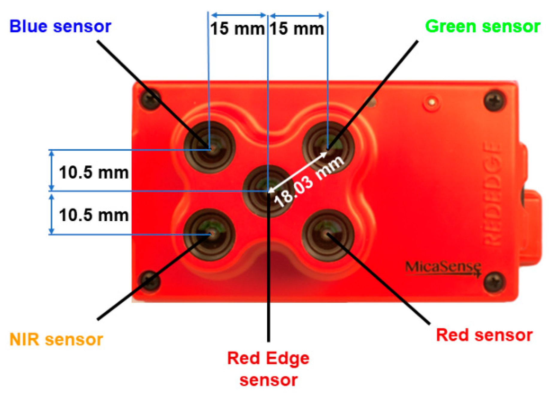
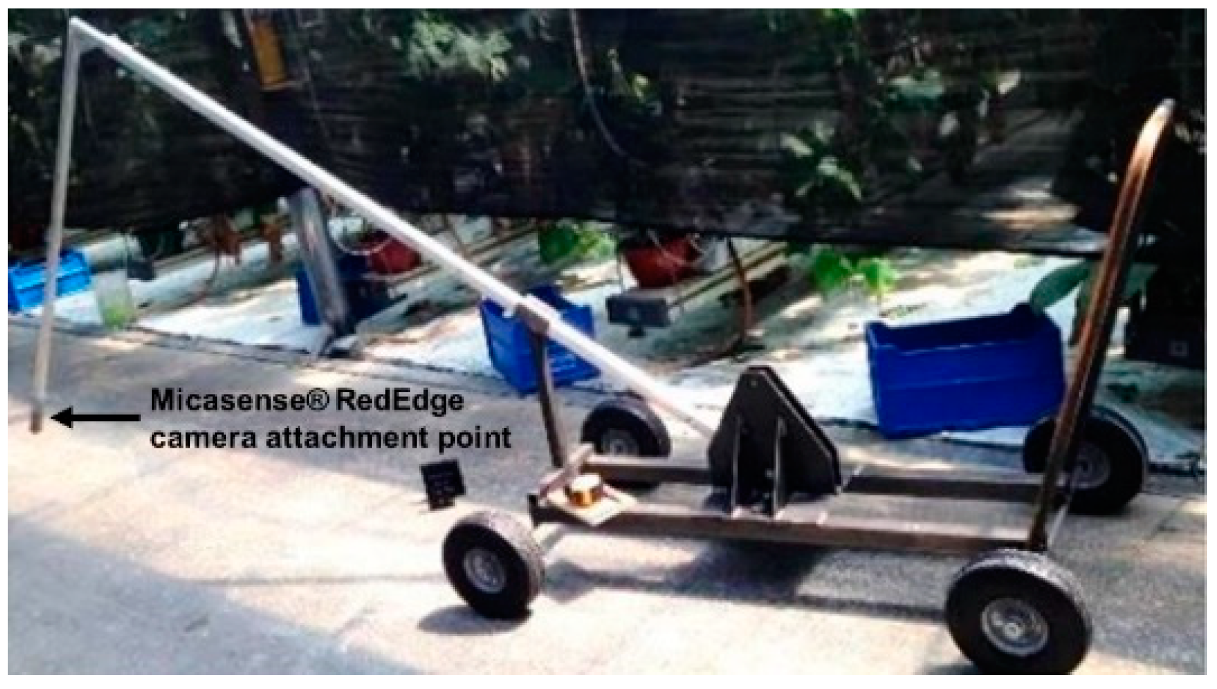
2.1. Image Acquisition

Forty-five multispectral images were collected with a MicaSense^® RedEdge camera over healthy and infected cucumber plants located in a greenhouse that belongs to Great Lakes Greenhouses Inc., a horticultural company, which is in Leamington, Canada (42°04′27″ N 82°35′15″ W). The MicaSense^® RedEdge camera has five bands (

Table 1. Spectral information of each band from the MicaSense^® RedEdge camera.

Band #	Spectral Region	Central Wavelength (nm)	Bandwidth (nm)
1	Blue	475	20
2	Green	560	20
3	Red	668	10
4	NIR	840	40
5	Red-edge	717	10

) and a horizontal and vertical field of view of 0.82 radian (47.2°) and 0.62 radian (35.4°), respectively. The camera was attached to a metal structure that was on a cart, which has wheels to facilitate its movement inside the greenhouse aisles (Figure 2).

The images were collected under greenhouse light without the use of artificial light. The height of the camera position was at close range (1.5 m) from the top of the cucumber plants. The images dimensions were 1280 × 960 pixels, and the pixel size was estimated being 0.10 cm, according to Equation (1):

$$\mathrm{pixsize} = \frac{2\ast H\ast \tan \left(FOVh∕2\right)}{1280}\times 100,$$

(1)

where,

pixsize = dimensions of the pixel size on each band image (cm);

H = camera position height (=1.5 m);

FOVh = horizontal field of view of the MicaSense^® RedEdge camera (0.82).

In order to cover the studied greenhouse area, more than one image had to be acquired over each row of plants. After capturing one image, the cart moved forward by a distance D to collect an image of a new section of the plant row. The process was repeated until all of the greenhouse area was surveyed. The distance (D) between two adjacent images on each row was computed according to Equation (2) as follows:

$$D = (1 - \mathrm{P}) \ast 2 \ast \mathrm{H} \ast tan\left(vFOV/2\right),$$

(2)

where

• D = camera displacement to image a new section of the plants row(m);
• P = overlap between images (10%);
• H = camera position height (m);
• vFOV = vertical field of view of the MicaSense^® RedEdge camera (0.62).

2.2. Image Processing

The workflow of the steps from the image acquisition to the computation of the root mean square error (RMSE) of registered images is presented in Figure 3. All data were processed using MATLAB R2020a (MathWorks, Inc., Natick, MA, USA). The information related to the MATLAB R2020a functions used in this study and their related parameters was obtained from www.mathworks.com. The collected images and their respective bands were imported into the MATLAB workspace and converted from uint16 to uint8 file formats using the im2uint8 function. Then, the first 700 columns were removed from each band because this image region was related to the aisle of the greenhouse. The images were then subjected to the image registration process which includes (i) SURF features detection and matching; (ii) geometric transformation; (iii) image wrapping; and (iv) computation of the RMSEs (in pixel) of the positions of the inliers matching points between the fixed and transformed moving images. In the study, we used the raw DN images without converting in reflectance values.

2.2.1. SURF Features

Point Detection

The first step of the image registration involves the detection of common features between the moving and fixed images. During this step, the blue, green, red, and NIR band images were used as moving images and the RedEdge band image as the reference (fixed) image because of its central location on the camera. We applied to the images the detectSURFFeatures function that is based on the SURF algorithm [25]. As detailed in Bay et al. [20], a Speeded-Up Robust Features (SURF) feature is an interest or key point in an image that has been detected and its neighborhood been described using the Speeded-Up Robust Features algorithm. The SURF feature corresponds to a blob-like structure as shown in Figure 4 for the blue, green, red, red-edge, and NIR band images.

The SURF algorithm detects the interest points using the Hessian matrix and it is why the point detection step of the SURF algorithm is also known as being the Fast-Hessian step. Specifically, the SURF algorithm detects blob-like structures at locations where the determinant of the Hessian matrix is maximum. Given a point x = (x, y) in an image I, the Hessian matrix $\mathcal{H}$ (x, σ) in x at scale σ is defined as [20]:

$$\mathcal{H}\left(x,\sigma \right)= \left[\begin{array}{cc}Lxx\left(x,\sigma \right)& Lxy\left(x,\sigma \right)\\ Lyx\left(x,\sigma \right)& Lyy\left(x,\sigma \right)\end{array}\right],$$

(3)

where, Lxx(x,σ), Lxy(x,σ), Lyx(x,σ), and Lyy(x,σ) are the convolutions of the Gaussian second-order derivative $\frac{{\partial }^2}{\partial x^2}g\left(\sigma \right)$ with the image I in point x.

The second-order Gaussian derivative is approximated using box filters that reduce computational time. Since the interest points need to be found at different scales, scale spaces need to be considered. They are usually implemented as an image pyramid. When the SURF algorithm is detecting interest points, the images are repeatedly smoothed with the Gaussian second-order derivatives that are approximated using box filters and then sub-sampled to achieve higher levels of the pyramid. The scale-space is analyzed by upscaling the box filter rather than iteratively reducing the image size. The scale space is divided into octaves. An octave represents a series of filter response maps obtained by convolving the same input image with a filter of increasing size. Each octave is subdivided into a constant number of scale levels. The construction of the scale space starts with the 9*9 filter, which calculates the blob response of the image for the smallest scale. Then, filters with sizes 15*15, 21*21, and 27*27 are applied. For each new octave, the filter size is doubled (i.e., from 6-12 to 24-48). At the same time, the sampling intervals for the extraction of the interest points can be doubled as well for every new octave. This reduces the computation time and the loss in accuracy. Finally, to localize interest points in the image, the algorithm applies a non-maximum suppression in a 3*3*3 neighborhood, corresponding to a fast variant of the efficient non-maximum suppression method of [26]. The maxima of the determinant of the Hessian matrix are then interpolated in scale and image space with the method proposed by [27].

The detectSURFFeatures function parameters were modified from their default values to obtain the highest possible number of blobs (

Table 2. Default and applied values of the parameters of the detectSURFFeatures function used in the registration of the images acquired with the MicaSense^® RedEdge camera.

Parameter	Default Value	Applied Value
MetricThreshold	1000	1
NumOctaves	3	4
NumScaleLevels	4	6

). The first function parameter is the MetricThreshold, which is a non-negative scalar. The value of this threshold can be reduced to return more blobs. The second parameter, NumOctaves (number of octaves) is defined by a scalar equal or greater than 1. Increasing the number of octaves allows for detecting larger blobs. The third parameter, NumScaleLevels (number of scale levels per octave), allows the detection of more blobs at finer scale increments if the parameter is equal or greater than 3.

Feature Extraction

Once the SURF features were obtained, we extracted feature descriptors and their corresponding locations on the moving and fixed images using the extractFeatures function. A feature descriptor is a feature vector describing the distribution of the intensity within the interest point neighborhood [28]. It depends on the orientation assignment and the sum of Haar wavelet responses. During the orientation assignment, the derivation of the descriptor is based on the distribution of the first order Haar wavelet responses in x and y directions within a radius of 6s around the interest point, where s is the scale at which the interest point was detected. This approach reduces the time for feature computation and matching, at the same time increasing the detector robustness. The dominant orientation is estimated by the sum of all responses within a sliding orientation window of size $\frac{\pi }{3}$. The horizontal and vertical responses within the window are summed. The resulting summed responses yield a local orientation vector. For extracting the descriptor, first, a square region centered on the interest point is constructed. The size of the square region is defined by 20s. This square region is divided into 4 × 4 subregions. For each sub-region, the algorithm computes the Haar wavelet responses at 5*5 regularly spaced sample points. The horizontal and vertical wavelet responses are summed up over each sub-region and form the first set of entries in the feature descriptor. To add information about the polarity of the intensity changes, the sum of absolute values of the horizontal and vertical wavelet responses are extracted. A descriptor vector having a specific length is achieved by concatenating the sum of horizontal and vertical wavelet responses and the sum of absolute values of the horizontal and vertical for all of the 4*4 sub-regions, as shown in Equation (4):

$$v=({\displaystyle \sum }dx, {\displaystyle \sum }\left|dx\right|,{\displaystyle \sum }dy,{\displaystyle \sum }\left|dy\right|)$$

(4)

where

• ${\displaystyle \sum }dx$ = the sum of horizontal the wavelet responses values for all of the 4*4 sub-regions;
• ${\displaystyle \sum }\left|dx\right|$= the sum of absolute horizontal wavelet responses values for all of the 4*4 sub-regions;
• ${\displaystyle \sum }dx$ = the sum of the vertical wavelet responses values for all of the 4*4 sub-regions;
• ${\displaystyle \sum }\left|dx\right|$ = the sum of the absolute vertical wavelet responses for all of the 4*4 sub-regions.

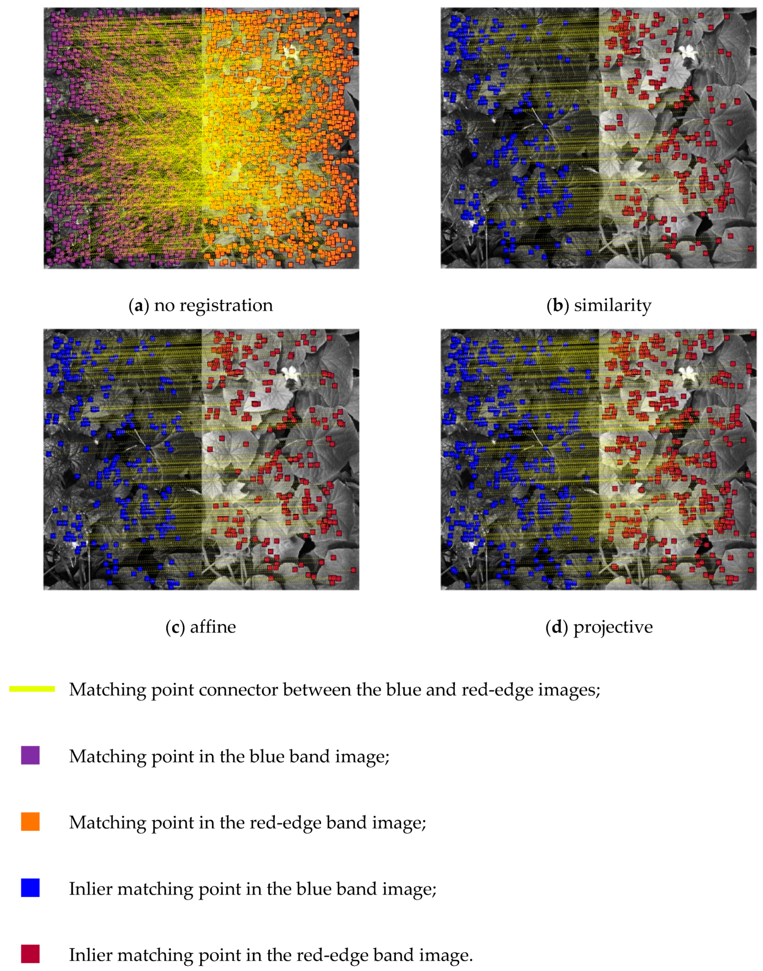
One extractFeatures function parameter, the FeatureSize parameter, which defines the length of the feature vector, was modified from 64 (default) to 128. According to Lowe [22] and Hassaballah et al. [23], high dimension feature vectors are more distinctive because features can be more correctly matched against a large set of features. Therefore, setting the FeatureSize parameter to 128 increases the accuracy of correctly matching interest points. To create a vector of length 128, the sums of dx and |dx| are computed separately for dy < 0 and dy ≥ 0. Then, the sums of dy and |dy| are split up according to the sign of dx, thereby doubling the number of features.

Matching Features

During the matching stage, the descriptor vectors are matched between the moving and fixed images. The matching is based on a distance between the vectors. The dimension of the descriptor has a direct impact on the time this step takes, and a low dimension is desirable for fast matching of interest points. Such matching features was performed with the matchFeatures function. The function has three parameters (

Table 3. Default and applied values of the parameters of the matchFeatures function used to register the MicaSense^® RedEdge images.

Parameter	Band	Default Value	Applied Value
MatchThreshold	All bands	10	50
MaxRatio	Blue–Red–NIR	0.60	0.90
	Green	0.60	0.75
Unique	All bands	false	true

). The first one is the MatchThreshold parameter that represents the percent of the distance from a perfect match. Two feature vectors match when the distance between them is less than the threshold set by the MatchThreshold parameter. The function rejects a match when the distance between the features is greater than the value of MatchThreshold. The second parameter is the MaxRatio parameter, which is a ratio threshold that allows rejecting ambiguous matches. The default values of this parameter allow detecting less than 500 matching points. To increase this number to 1100, the MaxRatio was set to 0.9 for the blue, red, and NIR bands and 0.75 for the green band. The third parameter is the Unique parameter that was set as true to perform a forward–backwards match that selects a unique match by keeping the best match between the features of the moving and fixed images.

2.2.2. Geometric Transformations

The image registration process involves a geometric transformation that allows transforming the moving image into the red-edge band space. It is based on the matching points of the moving and fixed images. Such transformation corrects the image distortions and allows band alignment. The ideal geometric transformation will remove only the spatial distortions between images [29]. The geometric transformation was done as follows. First, the M-estimator Sample Consensus (MSAC) algorithm embedded in the estimateGeometricTransform function was used to exclude outliers matching points [24]. The MSAC algorithm is a faster variant of the Random Sample Consensus (RANSAC) algorithm [30]. Removing outliers matching points allows reducing the percentage of alignment errors present in the total number of matching points to achieve a more accurate alignment. The MSAC algorithm is controlled by two function parameters. The MaxNumTrials (maximum random trials) parameter defines the maximum number of random trials for finding the inliers matching points. Increasing the MaxNumTrials value improves the MSAC algorithm fitting. Its default value was increased to 10,000 (

Table 4. Default and applied values of two parameters of the estimateGeometricTransform function used in this study.

Parameter	Projection	Default Value	Applied Value
MaxNumTrials	Affine, similarity, and projective	1000	10,000
MaxDistance	Affine and similarity	1.5	1.5
	Projective	1.5	3.0

). The second function parameter is the Confidence parameter, which determines the confidence of finding the maximum number of inliers. We used its default value of 99. Once the outliers are removed, the estimateGeometricTransform function creates a two-dimensional (2D) geometric transform object containing the geometric transformation matrix that defines the geometric transformation type through the TransformType parameter. We considered in this study all three available geometric transformations, i.e., affine, similarity, and projective. The similarity transformation is one of the simplest models and consists of rotation, scaling, and translation of the moving image [31,32]. The affine transformation is slightly more general than the similarity transformation and assumes that the distance of the camera to the scene is large in comparison to the size of the scanned area. The affine transformation matrix is defined by three non-collinear matching points and should be applied when shapes in the moving image exhibit shearing distortions [32]. The projective transformation is recommended when images are obtained at different view directions from the scene [33] or if the condition on the distance of the camera from the scene is not satisfied [32]. The geometric transformation is also controlled by the MaxDistance (maximum distance from a point to projection) parameter, which defines the maximum distance in pixels from a point to the projection of its corresponding point. We used the default value of 1.5 for the affine and similarity projections, but the value changed to 3.0 for the projective transformation that requires a higher distance to perform (Table 4).

To apply the geometric transformation to each moving image (blue, green, red, and NIR bands), we used the imwarp function with the respective T matrix computed with the estimateGeometricTransform function. The imwarp function returns the moving image transformed into the red-edge band space. The procedure was done for each transformation type (affine, similarity, projective).

2.2.3. RMSE Computation

The inliers matching point positions on both the fixed and transformed moving images were used to compute a root mean square error (RMSE) to assess the registration accuracy quantitatively. First, we used the transformPointsForward function to determine the pixel coordinates (in image rows and columns) of each inlier matching point on both images. The resulting coordinates were then plotted to visualize the displacement of the inliers matching points between the fixed and moving images for each transformation type. The RMSE (in pixels) between the positions of the inliers matching points on both the fixed and transformed moving images was then computed as follows (Equation (5)):

$$\mathrm{RMSE} = \sqrt{{{\displaystyle \sum }}_{\mathrm{i}=1}^{\mathrm{n}}\frac{{\left({\hat{\mathrm{x}}}_{\mathrm{i}}-{\mathrm{x}}_{\mathrm{i}}\right)}^2 + {\left({\hat{\mathrm{y}}}_{\mathrm{i}}-{\mathrm{y}}_{\mathrm{i}}\right)}^2 }{\mathrm{n}}}$$

(5)

where

${\hat{\mathrm{x}}}_{\mathrm{i}}$ = column number of the inlier matching point in the fixed (red-edge) image;

x_i = column number of the inlier matching point in the moving image (blue, green, red, and NIR images);

${\hat{\mathrm{y}}}_{\mathrm{i}}$ = row number of the inlier matching point in the fixed (red-edge) image;

y_i = row number of the inlier matching point in the moving image (blue, green, red, and NIR images);

RMSE= root mean square error for all of the inliers matching points of the moving image (in pixels).

The resulting RMSEs were then plotted using boxplots to compare the performance of each transformation. We also plotted the RMSEs distribution because according to Chai and Draxler [34], the RMSEs should have a Gaussian distribution rather than a uniform distribution.

3. Results

3.1. SURF Features

Figure 5 presents a comparison of the total number of matching points between the blue, green, red, and NIR bands (moving images) and the red-edge band (fixed image) for the 45 multispectral images acquired with the MicaSense^® RedEdge camera over the cucumber plants. The related descriptive statistics are given in

Table 5. Descriptive statistics as a function of the band for the number of matching points obtained using the SURF features method over the blue, green, red, and NIR band images (moving images) and the red-edge band images (fixed image) of 45 multispectral images acquired with the MicaSense^® RedEdge camera.

Band	Minimum	Maximum	Mean	Standard Deviation	Standard Error
Blue	1250	1599	1415.80	72.35	10.78
Green	1125	2089	1708.20	216.96	32.34
Red	1314	1670	1457.40	79.13	11.79
NIR	1383	1770	1579.80	96.38	14.36

. In general, the green band image (Figure 5) had a higher number of matching points with a mean matching points value of 1708.20 (Table 5), followed by the NIR band image (Figure 5) with a mean number of matching points of 1579.80 (Table 5). Both the blue and red band images (Figure 5) had similar mean values of the number of matching points, (1415.80 and 1457.40, respectively) (Table 5). However, the blue band image (Figure 5) had a lower standard deviation, and a lower standard error compares to the red band image (Table 5). Among all of the images, the green band image number 30 had the lowest number of matching points (Figure 5), with a value of 1125 (Table 5).

It is important to attempt reaching the higher possible number of matching points, before the geometric transformation, even if this increases the standard deviation. Indeed, we are registering images acquired in different wavelengths, therefore, we need to be able to match points across the whole moving and fixed band images. Even if a lower number of matching points with a lower standard deviation could produce better accuracy, this could lead to not detecting inliers matching points when the MSAC algorithm is applied, therefore, leading to a poor or null estimation of the T matrix that is used in the geometric transformation.

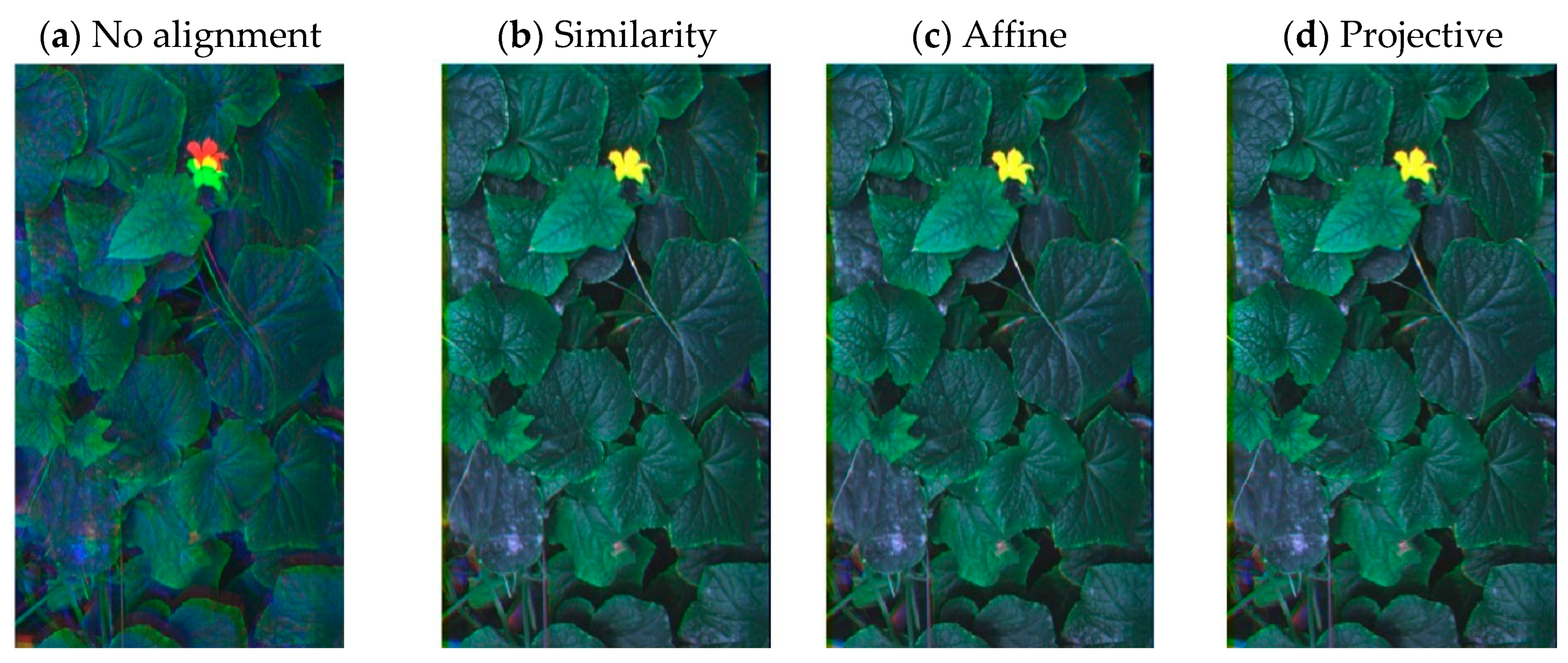
3.2. Geometric Transformation

Table 6. Descriptive statistics as a function of the band for the number of inliers matching points obtained using the SURF features and three geometric transformations over the blue, green, red, and NIR band images (moving images) and the red-edge band images (fixed image) in the case of 45 multispectral images acquired with the MicaSense^® RedEdge camera.

Geometric Transformation	Band	Min	Max	Mean	Standard Deviation	Standard Error	Mean Percentage (%) (1)
Similarity	Blue	78	282	162.40	45.27	6.74	11.39
	Green	318	1295	777.02	219	32.64	44.74
	Red	88	280	169.95	43.17	6.43	11.59
	NIR	124	413	210.26	54.95	8.19	13.22
Affine	Blue	73	274	171.06	46.75	6.96	11.99
	Green	347	1242	808.57	224.22	33.42	46.58
	Red	89	291	183.62	46.46	6.92	12.50
	NIR	130	367	225.95	57.77	8.61	14.21
Projective	Blue	136	444	292.20	64.78	9.65	20.52
	Green	622	1692	1273.50	245.95	36.66	73.97
	Red	165	457	320.84	67.05	9.99	21.89
	NIR	249	672	414.17	94.57	14.19	26.05

(1) With respect to the total number of matching points.

compares the descriptive statistics for the number of inliers matching points obtained after the feature detection, extraction, and matching using SURF features in the case of the three transformation methods. The projective transformation had a higher mean number of inliers matching points for all bands than the two other transformations. (Table 6). For all of the transformations, the highest mean number of inliers matching points was obtained for the green band image followed by the NIR band image. The mean number of inliers for the blue band and red band images were the lowest. The affine and similarity transformations presented similar statistics (Table 6). However, the magnitudes of the statistics for the affine transformation were slightly higher than those computed for the similarity transformation.

Figure 6 presents the percentage of inliers matching points with respect to the total number of matching points. The MSAC algorithm reduced the total number (percentage) of matching points for the blue band, by 1244 (87.91%) and 1253 (88.53%) for the affine and similarity transformations, respectively, for the green band, by 899 (52.66 %) and 931 (54.51%) for the affine and similarity transformations, respectively, for the red band, by 1273 (87.40%) and 1287 (88.33%) for the affine and similarity transformations, respectively, and for the NIR band, by 1353 (85.69%) and 1369 (86.69%) for the affine and similarity transformations, respectively (Figure 6). However, when applying the MSAC algorithm with the projective transformation, the number of total matching points for the blue, green, red, and NIR bands was reduced approximately by 1123 (79.36%), 434 (25.44%), 1136 (77.98%), and 1165 (73.78%), respectively (Figure 6).

A visual comparison of the distribution of the total number of matching points and the new set of inliers matching points between the moving images and the fixed image is presented in Figure 7, Figure 8, Figure 9 and Figure 10 for the blue, green, red, and NIR bands, respectively. For the blue band image (Figure 7), the points are distributed over the whole area of the image (Figure 7). The projective transformation over the blue band showing a better distribution of the matching points by keeping the points at the right edge of the image and a few in the left bottom corner (Figure 7). However, for the similarity and affine transformations, the number of inliers matching points for the blue band is reduced in the right edge and in the lower-left corner of the image (Figure 7). In the green band, all of the matching points are well distributed over the image (Figure 8). Both the similarity and projective transformations presented a good distribution of the inliers matching points over the edges and center of the images. However, the affine transformation missed to include matching points in the left bottom corner of the image (Figure 8). The red band image presented a different distribution for the three transformations (Figure 9). Ideally, the matching points should be well distributed. However, the similarity transformation (Figure 9) failed to determine matching points in the right top corner and near the right edge of the image. It is also noticed that the similarity transformation did not find inliers matching points in the left central side of the image (Figure 9). The results for the affine transformation in the red band image were like the ones of the similarity transformation (Figure 9), which missed matching points in the right edge of the image. However, the affine transformation included a higher number of matching points distributed in the left central area of the image, including one in the left bottom corner. With the projective transformation (Figure 9), the inliers matching points had a better spatial distribution over the image. It is also possible to observe a few matching points in the top right area of the image and on the right edge. The projective transformation also has a higher number and distribution of matching points in the left-center area of the images (Figure 9).

Finally, for the NIR band image (Figure 10) it is possible to observe that most of the original matching points located in the edges were removed when the similarity transformation was applied (Figure 10). The affine transformation presented a similar matching point distribution as the similarity transformation (Figure 10). With the affine transformation, some matching points were kept in the nearest location to the left edge of the image, but failed to keep matching points in the left bottom corner of the image (Figure 10). The projective transformation improved slightly the distribution of the matching points by including the left bottom corner of the image and placing some matching points near to the left and right edges of the images (Figure 10). However, the projective transformation missed points in the top right corner of the image (Figure 10). The resulting RGB composite images after applying the imwarp function are presented in Figure 11. All three transformation types produce good alignment, but some blurry regions can be observed in the left lower corner of each image (Figure 11).

The computation time of each of the main processes of the image registration is presented in

Table 7. Image registration computation time for each function in the case of 45 multispectral images acquired with the MicaSense^® RedEdge camera.

Function	Geometric Transformation	Time (s)	Cumulative time (s)			Average Time Per Band (1)
detectSURFFeatures		14.18	14.18			0.079
extractSURFFeatures		18.62	32.80			0.182
matchFeatures		114.77	147.57			0.820
estimateGeometricTransform	Affine	144.55	292.13			1.623
	Similarity	16.81		164.38		0.913
	Projective	224.77			372.35	2.069
imwarp	Affine	0.83	292.95			0.005
	Similarity	0.75		165.13		0.004
	Projective	1.87			374.22	0.010

(1) Based on a total number of moving band images of 180.

. The computation time to detect the SURF features was 14.18 s, the one to extract the SURF features was 18.62 s, and the one to match the features was 114.77 s. The time to apply the estimateGeometricTransform function for obtaining the T matrix and inliers matching points depends on the geometric transformation type. It was 144.55 s for the affine transformation, 16.81 s for the similarity transformation, and 224.77 s for the projective transformation. The image registration with the imwarp function was the fastest process, lasting only 0.83 s, 0.75 s, and 1.87 s with the similarity, affine, and projective transformations, respectively (Table 7). Overall, the fastest registration method was the one using the similarity transformation (165.13 s) followed by the one using the affine transformation (292.95 s) and then the one using the projective transformation (374.22 s) (Table 7). Table 7 also gives the mean time per band for each process, given that the method was applied to 180 moving bands, i.e., 45 blue band images, 45 green band images, 45 red band images, and 45 NIR band images).

3.3. RMSE

To provide a quantitative metric to assess the performance of each image registration, RMSEs of the inliers matching points between the moving and reference images were computed for each transformation and each band. The resulting RMSEs were plotted in boxplots that show that the projective transformation presented the highest RMSE for all of the band images, with an RMSE value near 1.5 pixels (Figure 12). The corresponding RMSEs were less than 1 pixel with the similarity and affine transformations (Figure 12). Figure 13 presents the distribution of the RMSE as a function of the band and image transformation. The best image registration method should be as such that the RMSEs have a Gaussian distribution because model errors are likely to have a Gaussian distribution rather than a uniform distribution [34]. With the affine transformation, RMSEs have a Gaussian distribution for all of the band images, except for the blue band image.

4. Discussion

Our study aims to develop a method that allows the registration of non-georeferenced close-range multispectral images acquired with a MicaSense^® RedEdge camera over greenhouse cucumber healthy and infected plants. In order to be suitable for disease detection, the developed method should properly align the various band images in order to be able to integrate the spectral information from the different band images to gain more complex and detailed scene representation [32]. Image registration is generally done by registering one image (moving image) as a function of another one (fixed image). Since there is no defined method to select the reference image during image registration [35], we defined the red-edge band image as the fixed reference image in this study because the red-edge sensor of the MicaSense^® RedEdge camera is located at the center of the sensor (Figure 1). Such definition allows keeping similar spatial misalignment among the other band images, i.e., the blue, green, red, and NIR band images which are here the moving images, i.e., images to be registered.

Such image registration requires determining matching points that represent the same features on the moving and fixed images. The detected feature sets in the moving and fixed image must have enough common elements [32]. We applied the detectSURFFeatures function to detect SURF features. SURF features have been designed to determine mapping key points between two images on the assumption that corresponding key points have a similar gradient pattern around them [36]. The parameters of the detectSURFFeatures function were modified to obtain the highest possible number of matching points, given that a high number of points is required with high-resolution images [37]. We observed that the highest number of matching points were detected in the green band image (2089), followed by the NIR band image (1770) and the blue and red band images (1599 and 1670, respectively). We cannot attribute the highest number of total matching points for the green band to the modified parameters of the matchFeatures function, because the highest number for the green band is also observed with the default values of the function parameters. The highest number in the green band should also not be related to the SURF algorithm we used. Indeed, this result was also observed by Yasir et al. [38] who registered MicaSense^® RedEdge green, red and NIR images into the RedEdge space with a data-driven algorithm. It was also observed by Hassanpour et al. [39] who registered MicaSense^® RedEdge green, red and NIR images with a Patch-Wise and Local Window registration method. The higher number of total matching points for the green and NIR band images compared to the blue and red band images is probably related to the fact that the green and NIR images are related to high DN values because they were acquired over green vegetation that reflects the most in the green and NIR wavelengths by contrast to the blue and red band images that correspond to the chlorophyll absorption bands which produce low DN values.

Given that the matching points obtained from feature points are prone to be unstable and produce many mismatches, it is necessary to remove outliers from the initial matching point set before a geometric transformation is applied [38]. The outliers were removed using the MSAC algorithm. The MSAC algorithm reduced the total number of matching points by 1244 and 1253 for the affine and similarity transformations, respectively in the case of the blue band image, by 900 and 931 for the affine and similarity transformations, respectively in the case of the green band image, by 1274 and 1288 for the affine and similarity transformations, respectively, in the case of the red band image and by1353 and 1369 for the affine and similarity transformations, respectively in the case of the NIR band image. However, when applying the MSAC algorithm with the projective transformation, the number of total matching points for the blue, green, red, and NIR band images was reduced approximately by 1123, 473, 1137, and 1165, respectively.

Despite these reductions, whatever the geometric transformation, the resulting number of matching points was higher than those reported by Yasir et al. [38] who reported 81, 282, 195, and 134 matching points for the blue, green, red, and NIR bands respectively, when applying a data-driven registration algorithm to images acquired with the MicaSense RedEdge camera over greenhouse canola plants.

The resulting matching points were then used to compute the RMSE associated with each image transformation and band image. Kerkech et al. [40] reported that a disease detection system using multispectral images should perform better if the RMSE of the image registration process is less than 5 pixels, given that RMSEs between 5 and 10 pixels may reduce the accuracy of disease localization in some cases. We achieved an RMSE of less than 1 pixel with the similarity and affine transformations and of less than 2 pixels with the projective transformation, whatever the band image. Our RMSEs were lower than those (higher than 2.5 pixels) obtained by Hadaddi and Leblon [41] who performed image registration and band alignment on the same non-georeferenced multispectral MicaSense^® RedEdge images as our study. There are several differences between our study and Haddadi and Leblon [33]. First, Haddadi and Leblon [33] located the matching points with the Harris corner detector [42] and the Scale Invariant Feature Transform (SIFT) algorithm [22], while in our case, we used the SURF features detector and the matchfeatures function of MATLAB (R2020a). Secondly, they used the green band image as the reference image, while in our study, we selected the red-edge band image that is more centrally located. Thirdly, a quadratic polynomial transformation was used as a geometric transformation [43], while our study evaluated three geometric transformations (affine, similarity, and projective). Our RMSEs were also lower than those reported by Wang et al. [44] (0, 28.64, and 69.16 pixels) who applied three area-based registration methods over thermal and optical RGB images. Our study used a feature-based image registration approach, while Wang et al. [43] used area-based registration methods. According to Chai and Draxler [34], the best registration method should be such that the RMSEs have a Gaussian distribution because model errors are likely to have a Gaussian distribution rather than a uniform distribution. Our results showed that with the affine transformation, all of the bands, but the blue band, the RMSEs had a Gaussian distribution.

5. Conclusions

In this study, we evaluated three methods of image registration in the case of non-georeferenced multispectral images acquired at close range over greenhouse cucumber plants with a MicaSense^® RedEdge camera attached to a mechanic extension of a mobile cart. The registration method includes the detection of matching points between the moving and fixed images and the application of a geometric transformation for band alignment. The three methods use the blue, green, red, and NIR bands as moving images and the red-edge band as the fixed reference image because the related sensor has a central position. In each case, the detection of matching points was performed using SURF features. We considered three geometric transformations (affine, similarity, and projective). For each transformation, we mapped the matching points of the blue, green, red, and NIR bands into the red-edge band space and computed the root mean square error (RMSE in pixel) to assess the accuracy of the image registration. Our results showed that the affine transformation is the best approach for image registration because, the RMSEs were less than 1 pixel and have a Gaussian distribution for all of the band images, but the blue band.

Our results were based on 45 non-georeferenced multispectral images acquired at close range over mature cucumber plants with a MicaSense^® RedEdge camera. Future research under greenhouse conditions should investigate whether the size of the canopy and leaf areas influence the accuracy of the image registration and band alignment, given that our study shows that the green and NIR band images have more matching points because it corresponds to high reflectance bands. Such tests can be done using younger cucumber plants that have low leaf areas. While the results of this study are quite promising, they were acquired on a limited number of images. Further work is needed to test the method of broad sampling.

References

1. Statistics Canada. 2017a. Available online: https://www.agr.gc.ca/eng/horticulture/horticulture-sector-reports/statistical-overview-of-the-canadian-greenhouse-vegetable-industry-2017/?id=1549048060760 (accessed on 26 November 2020).
2. Khater, M.; De La Escosura-Muñiz, A.; Merkoçi, A. Biosensors for plant pathogen detection. Biosens. Bioelectron. 2017, 93, 72–86. [Google Scholar] [CrossRef] [PubMed] [Green Version]
3. Hafez, Y.M.; Attia, K.A.; Kamel, S.M.; Alamery, S.F.; El-Gendy, S.; Al-Doss, A.A.; Mehiar, F.; Ghazy, A.I.; Ibrahim, E.I.; Abdelaal, K.A.A. Bacillus subtilis as a bioagent combined with nano molecules can control powdery mildew disease through histochemical and physiobiochemical changes in cucumber plants. Physiol. Mol. Plant Pathol. 2020, 111, 101489. [Google Scholar] [CrossRef]
4. Spanu, P.D.; Panstruga, R. Editorial: Biotrophic Plant-Microbe Interactions. Front. Plant Sci. 2017, 8. [Google Scholar] [CrossRef] [PubMed] [Green Version]
5. Nishizawa, Y.; Mochizuki, S.; Yokotani, N.; Nishimura, T.; Minami, E. Molecular and cellular analysis of the biotrophic interaction between rice and Magnaporthe oryzae–Exploring situations in which the blast fungus controls the infection. Physiol. Mol. Plant Pathol. 2016, 95, 70–76. [Google Scholar] [CrossRef]
6. Eskandari, S.; Sharifnabi, B. The modifications of cell wall composition and water status of cucumber leaves induced by powdery mildew and manganese nutrition. Plant Physiol. Biochem. 2019, 145, 132–141. [Google Scholar] [CrossRef]
7. Knipling, E.B. Physical and physiological basis for the reflectance of visible and near-infrared radiation from vegetation. Remote Sens. Environ. 1970, 1, 155–159. [Google Scholar] [CrossRef]
8. Atole, R.R.; Park, D. A multiclass deep convolutional neural network classifier for detection of common rice plants anomalies. Int. J. Adv. Comput. Sci. Appl. 2018, 9, 67–70. [Google Scholar]
9. Özgüven, M.M.; Adem, K. Automatic detection and classification of leaf spot disease in sugar beet using deep learning algorithms. Phys. A Stat. Mech. Appl. 2019, 535, 122537. [Google Scholar] [CrossRef]
10. Yang, C. Remote Sensing and Precision Agriculture Technologies for Crop Disease Detection and Management with a Practical Application Example. Engineering 2020, 6, 528–532. [Google Scholar] [CrossRef]
11. Jung, J.; Maeda, M.; Chang, A.; Bhandari, M.; Ashapure, A.; Landivar, J. The potential of remote sensing and artificial intelligence as tools to improve the resilience of agriculture production systems. Curr. Opin. Biotechnol. 2021, 70, 15–22. [Google Scholar] [CrossRef]
12. Bai, X.; Li, X.; Fu, Z.; Lv, X.; Zhang, L. A fuzzy clustering segmentation method based on neighborhood grayscale information for defining cucumber leaf spot disease images. Comput. Electron. Agric. 2017, 136, 157–165. [Google Scholar] [CrossRef]
13. Ma, J.; Du, K.; Zhang, L.; Zheng, F.; Chu, J.; Sun, Z. A segmentation method for greenhouse vegetable foliar disease spots images using color information and region growing. Comput. Electron. Agric. 2017, 142, 110–117. [Google Scholar] [CrossRef]
14. Zhang, S.; Wu, X.; You, Z.; Zhang, L. Leaf image based cucumber disease recognition using sparse representation classification. Comput. Electron. Agric. 2017, 134, 135–141. [Google Scholar] [CrossRef]
15. Zhang, S.; Zhang, S.; Zhang, C.; Wang, X.; Shi, Y. Cucumber leaf disease identification with global pooling dilated convolutional neural network. Comput. Electron. Agric. 2019, 162, 422–430. [Google Scholar] [CrossRef]
16. Kuppala, K.; Sandhya, B.; Barige, T.R. An overview of deep learning methods for image registration with focus on feature-based approaches. Int. J. Image Data Fusion 2020, 11, 113–135. [Google Scholar] [CrossRef]
17. Dawn, S.; Saxena, V.; Sharma, B. Remote sensing image registration techniques: A survey. In Proceedings of the Image and Signal Processing, 4th International Conference, ICISP, Trois-Rivières, QC, Canada, 30 June–2 July 2010; pp. 103–112. [Google Scholar]
18. Goshtasby, A.A. Image Registration Principles Tools and Methods, 1st ed.; Springer: London, UK, 2012; pp. 7–31. [Google Scholar]
19. Bay, H.; Tuytelaars, T.; Van Gool, L. SURF: Speeded Up Robust Features. In Proceedings of the 9th European Conference on Computer Vision (ECCV 2006), Graz, Austria, 7–13 May 2006; pp. 404–417. [Google Scholar]
20. Bay, H.; Ess, A.; Tuytelaars, T.; Van Gool, L. Speeded-Up Robust Features (SURF). Comput. Vis. Image Underst. 2008, 110, 346–359. [Google Scholar] [CrossRef]
21. Tareen, S.A.K.; Saleem, Z. A comparative analysis of SIFT, SURF, KAZE, AKAZE, ORB, and BRISK. In Proceedings of the Inter-national Conference on Computing, Mathematics and Engineering Technologies (iCoMET 2018), Sukkur, Pakistan, 3–4 March 2018; pp. 1–10. [Google Scholar]
22. Lowe, D.G. Distinctive Image Features from Scale-Invariant Keypoints. Int. J. Comput. Vis. 2004, 60, 91–110. [Google Scholar] [CrossRef]
23. Hassaballah, M.; Alshazly, H.; Ali, A.A. Analysis and Evaluation of Keypoint Descriptors for Image Matching. In Recent Advances in Computer Vision, Studies in Computational Intelligence; Hassaballah, M., Hosny, K., Eds.; Springer: Cham, Switzerland, 2019; Volume 854, pp. 113–140. [Google Scholar]
24. Torr, P.H.S.; Zisserman, A. MLESAC: A new robust estimator with application to estimating image geometry. Comput. Vis. Image Underst. 2000, 78, 138–156. [Google Scholar] [CrossRef] [Green Version]
25. Liu, J.; White, J.M.; Summer, R.M. Automated detection of blob structures by hessian analysis and object scale. In Proceedings of the 2010 IEEE 17th International Conference on Image Processing, Hong Kong, China, 26–29 September 2010; pp. 841–844. [Google Scholar]
26. Neubeck, A.; Van Gool, L. Efficient Non-Maximum Suppression. In Proceedings of the 18th International Conference on Pattern Recognition (ICPR’06), Hong Kong, China, 20–24 August 2006; pp. 850–855. [Google Scholar]
27. Brown, M.; Lowe, D. Invariant Features from Interest Point Groups. In Proceedings of the 13th British Machine Vision Confer-ence (BMVC 2002), Cardiff, UK, 2–5 September 2002; pp. 25.1–26.10. [Google Scholar]
28. Hassaballah, M.; Ali, A.A.; Alshazly, H. Image features detection, description, and matching. In Image Feature Detectors and Descriptors: Foundations and Applications; Awad, A., Hassaballah, M., Eds.; Springer: Cham, Switzerland, 2016; Volume 630, pp. 11–45. [Google Scholar]
29. Dai, X.; Khorram, S. A feature-based image registration algorithm using improved chain-code representation combined with Invariant Moments. IEEE Trans. Geosci. Remote Sens. 1999, 37, 2351–2362. [Google Scholar] [CrossRef] [Green Version]
30. Fischler, M.A.; Bolles, R.C. Random sample consensus: A paradigm for model fitting with applications to image analysis and automated cartography. Commun. ACM 1981, 24, 381–395. [Google Scholar] [CrossRef]
31. Szeliski, R. Image alignment and stitching: A tutorial. Found. Trends Comput. Graph. Vis. 2006, 2, 1–104. [Google Scholar] [CrossRef]
32. Zitová, B.; Flusser, J. Image registration methods: A survey. Image Vision. Comput. 2003, 21, 977–1000. [Google Scholar] [CrossRef] [Green Version]
33. Goshtasby, A.A. Piecewise linear mapping functions for image registration. Pattern Recognit. 1986, 19, 459–466. [Google Scholar] [CrossRef]
34. Chai, T.; Draxler, R. Root mean square error (RMSE) or mean absolute error (MAE)?—Arguments against avoiding RMSE in the literature. Geosci. Model Dev. 2014, 7, 1247–1250. [Google Scholar] [CrossRef] [Green Version]
35. Jin, H.; Fan, C.; Li, Y.; Xu, L. A novel coarse-to-fine method for registration of multispectral images. Infrared Phys. Technol. 2016, 77, 219–225. [Google Scholar] [CrossRef]
36. Hong, G.; Zhang, Y. Wavelet-based range image registration technique for high-resolution remote sensing images. Comput. Geosci. 2008, 34, 1708–1720. [Google Scholar] [CrossRef]
37. Zheng, J.; Xu, Q.; Zhai, B.; Wang, Y. Accurate hyperspectral and infrared satellite image registration method using structured topological constraints. Infrared Phys. Technol. 2020, 104, 103122. [Google Scholar] [CrossRef]
38. Yasir, R.; Eramian, M.; Stavness, I.; Shirtliffe, S.; Duddu, H. Data-driven multispectral image registration. In Proceedings of the 2018 15th Conference on Computer and Robot Vision (CRV), Toronto, ON, Canada, 8–10 May 2018; pp. 230–237. [Google Scholar]
39. Hassapour, M.; Javan, F.D.; Azizi, A. Band to band registration of multi-spectral aerial imagery-relief displacement and miss-registration error. In Proceedings of the International Archives Photogrammetry, Remote Sensing, and Spatial Information Sciences, GeoSpatial Conference, Karaj, Iran, 12–14 October 2019; Volume 42, pp. 467–474. [Google Scholar]
40. Kerkech, M.; Hafiane, A.; Canals, R. Vine disease detection in UAV multispectral images using optimized image registration and deep learning segmentation approach. Comput. Electron. Agr. 2020, 174, 105446. [Google Scholar] [CrossRef]
41. Haddadi, A.; Leblon, B. Developing a UAV-Based Camera for Precision Agriculture, Final Report; Mitacs # IT07423 Grant; University of New Brunswick: Fredericton, NB, Canada, 2018; 106p. [Google Scholar]
42. Harris, C.; Stephens, M. A combined corner and edge detector. In Proceedings of the 4th Alvey Vision Conference, Manchester, UK, 31 August–2 September 1988; pp. 147–151. [Google Scholar]
43. Schowengerdt, R.A. Remote Sensing: Models and Methods for Image Processing, 3rd ed.; Academic Press: Burlington, MA, USA, 2007; pp. 285–354. [Google Scholar]
44. Wang, X.; Yang, W.; Wheaton, A.; Cooley, N.; Moran, B. Efficient registration of optical and IR images for automatic plant water stress assessment. Comput. Electron. Agric. 2010, 74, 230–237. [Google Scholar] [CrossRef]
Figure 1. Figure showing the distance between the five sensors of the MicaSense® RedEdge camera (adapted from www.dronenerds.com).
Remotesensing 13 00396 g001
Figure 2. Mobile cart and adjustable metallic extension indicating the point where the MicaSense® RedEdge camera was placed to collect multispectral images over cucumber plants inside a greenhouse.
Remotesensing 13 00396 g002
Figure 3. Flowchart of the image registration methodology used in this study to register close-range non-georeferenced images acquired with the MicaSense® RedEdge multispectral camera over cucumber plants.
Remotesensing 13 00396 g003
Figure 4. Comparison of the blob-like structures detected over (a) blue, (b) green (c) red, (d) RedEdge, and (e) NIR band images acquired with a MicaSense® RedEdge camera at close range over cucumber plants.
Remotesensing 13 00396 g004
Figure 5. Variation as a function of the image number of the total number of matching points between the MicaSense® RedEdge blue, green, red, or NIR band images and the red-edge band image. The points were extracted using the Speeded-Up Robust Features (SURF) features algorithm.
Remotesensing 13 00396 g005
Figure 6. Variation as a function of the image number of the percentage of inliers matching points with respect to the total number of matching points for the MicaSense® RedEdge blue, green, red, and NIR band images that were subjected to the following geometric transformations: similarity, affine, and projective.
Remotesensing 13 00396 g006
Figure 7. Comparison between the distribution of the total number of matching points and the inliers matching points for the MicaSense® RedEdge blue and red-edge band images in the case of the following geometric transformations: no registration (a), similarity (b), affine (c), and projective (d). Outliers matching points were detected using the M-estimator Sample Consensus (MSAC) algorithm.
Remotesensing 13 00396 g007
Figure 8. Comparison between the distribution of the total number of matching points and the inliers matching points for the MicaSense® RedEdge green and red-edge band images in the case of the following geometric transformations: no registration (a), similarity (b), affine (c), and projective (d). Outliers matching points were detected using the M-estimator Sample Consensus (MSAC) algorithm.
Remotesensing 13 00396 g008
Figure 9. Comparison between the distribution of the total number of matching points and the inliers matching points for the MicaSense® RedEdge red and red-edge band images in the case of the following geometric transformations: no registration (a), similarity (b), affine (c), and projective (d). Outliers matching points were detected using the M-estimator Sample Consensus (MSAC) algorithm.
Remotesensing 13 00396 g009
Figure 10. Comparison between the distribution of the total number of matching points and the inliers matching points for the MicaSense® RedEdge near-infrared and red-edge band images in the case of the following geometric transformations: no registration (a), similarity (b), affine (c), and projective (d). Outliers matching points were detected using the M-estimator Sample Consensus (MSAC) algorithm.
Remotesensing 13 00396 g010
Figure 11. Comparison of the RGB composite created with the MicaSense® RedEdge blue, green, and red band images acquired at close range over cucumber plants. The image registration was achieved using the following geometric transformation (a) no registration, (b) similarity, (c) affine, (d) projective.
Remotesensing 13 00396 g011
Figure 12. Variation of the root mean square error (RMSE in pixels) computed for the inliers matching points as a function of the geometric transformation that was used to transform the blue (a), green (b), red (c), and NIR (d) band moving image into the fixed (red-edge band) image space.
Remotesensing 13 00396 g012
Figure 13. Distribution of the root mean square error (RMSE) computed for the inliers matching points after a forward transformation to the fixed (red-edge band) image space as a function of the transformation. The red line represents a Gaussian distribution. In order to improve visualization, the range of the x-axis was modified for the projective transformation.
Remotesensing 13 00396 g013