
Green LAI Mapping and Cloud Gap-Filling Using Gaussian Process Regression in Google Earth Engine

 , ,
, , 
Abstract
1. Introduction
2. Methodology
2.1. GPR Formulation for Vector Input
- Length-scale describes the smoothness of dependence along the dimension b. Small means changes quickly for variations of along b; large values denote slow changes w.r.t. the b dimension. Alternatively, the inverse of represents the relevance of band b in the prediction process. Intuitively, high values of mean that relations largely extend along that band hence suggesting a lower informative content.
- Signal variance is a scaling factor. It determines variation of from its mean. Small value of characterize functions that stay close to their mean value, larger values allow more variation. If is too large, the modeled function will be free to chase outliers.
- Noise variance is formally not a part of the covariance function itself. It is used by the Gaussian process model to account for noise present in training data.
2.2. GPR Formulation for Space-Spectrum (3D) Input
2.3. GPR Formulation for Space-Time (3D) Input
3. GPR Models Training
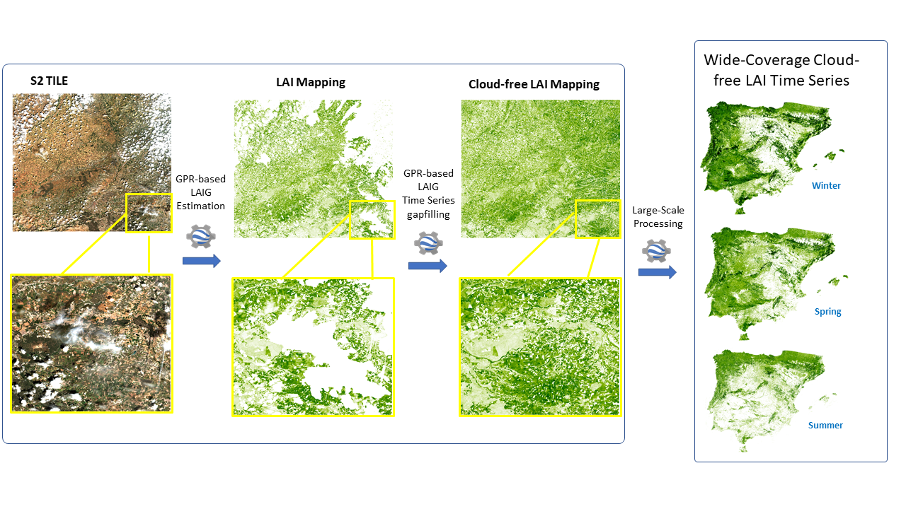
3.1. Green LAI Model
3.2. Gapfilling Model
4. GEE Implementation and Assessment
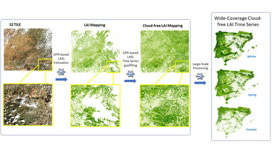
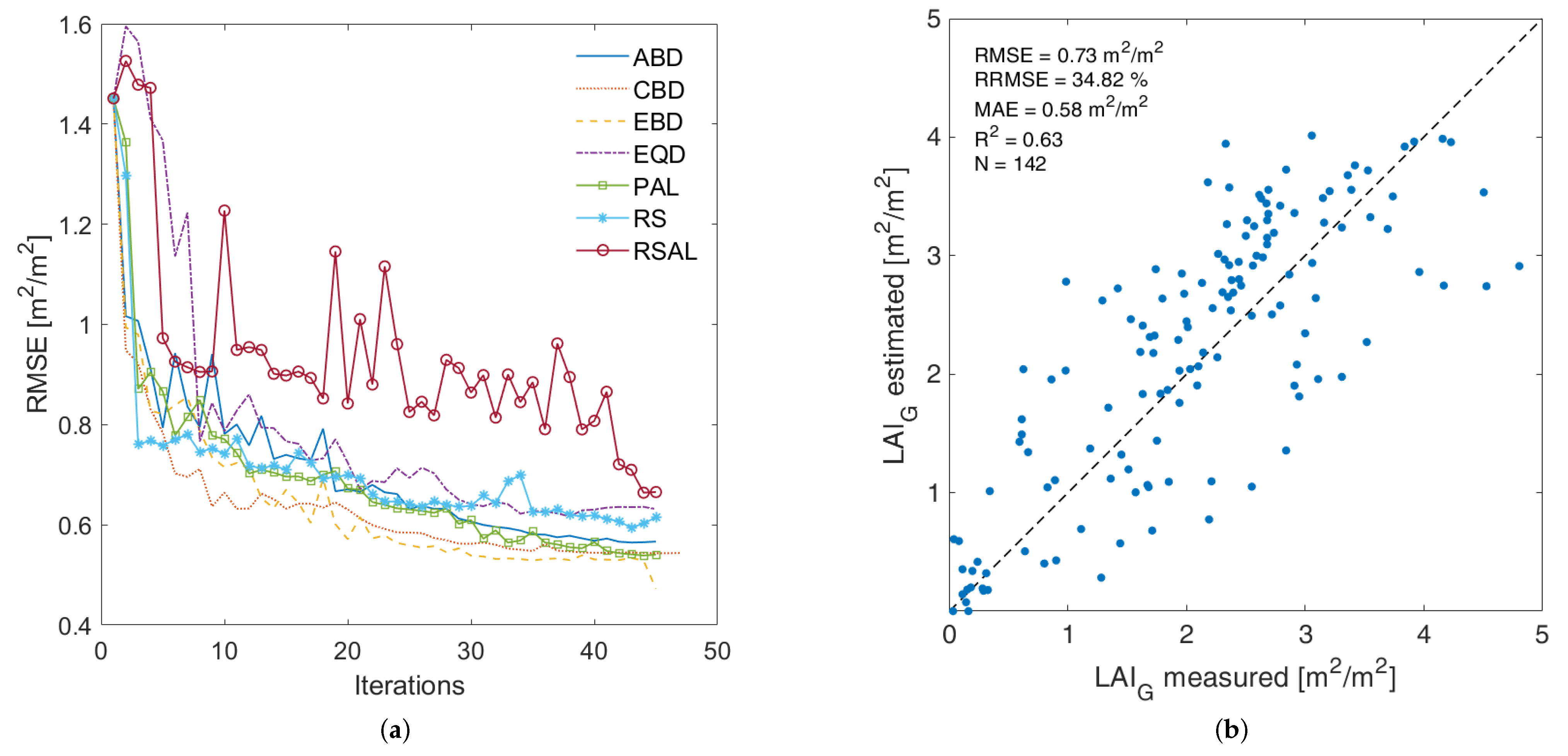
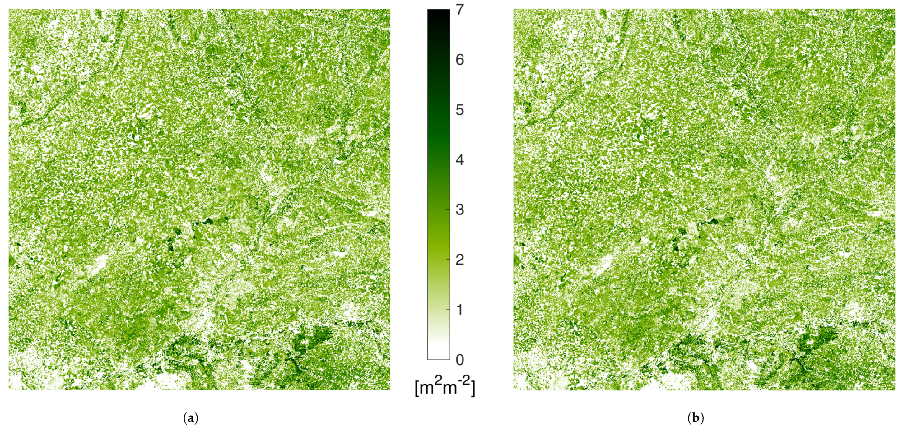
4.1. LAI Mapping
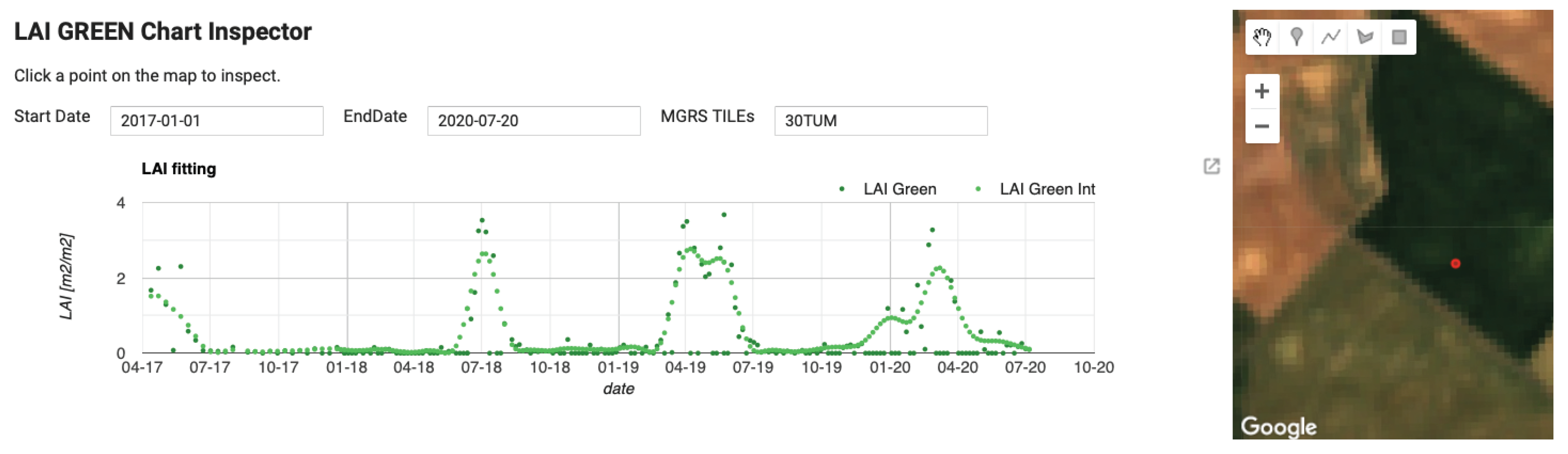
4.2. LAI Time Series Gapfilling
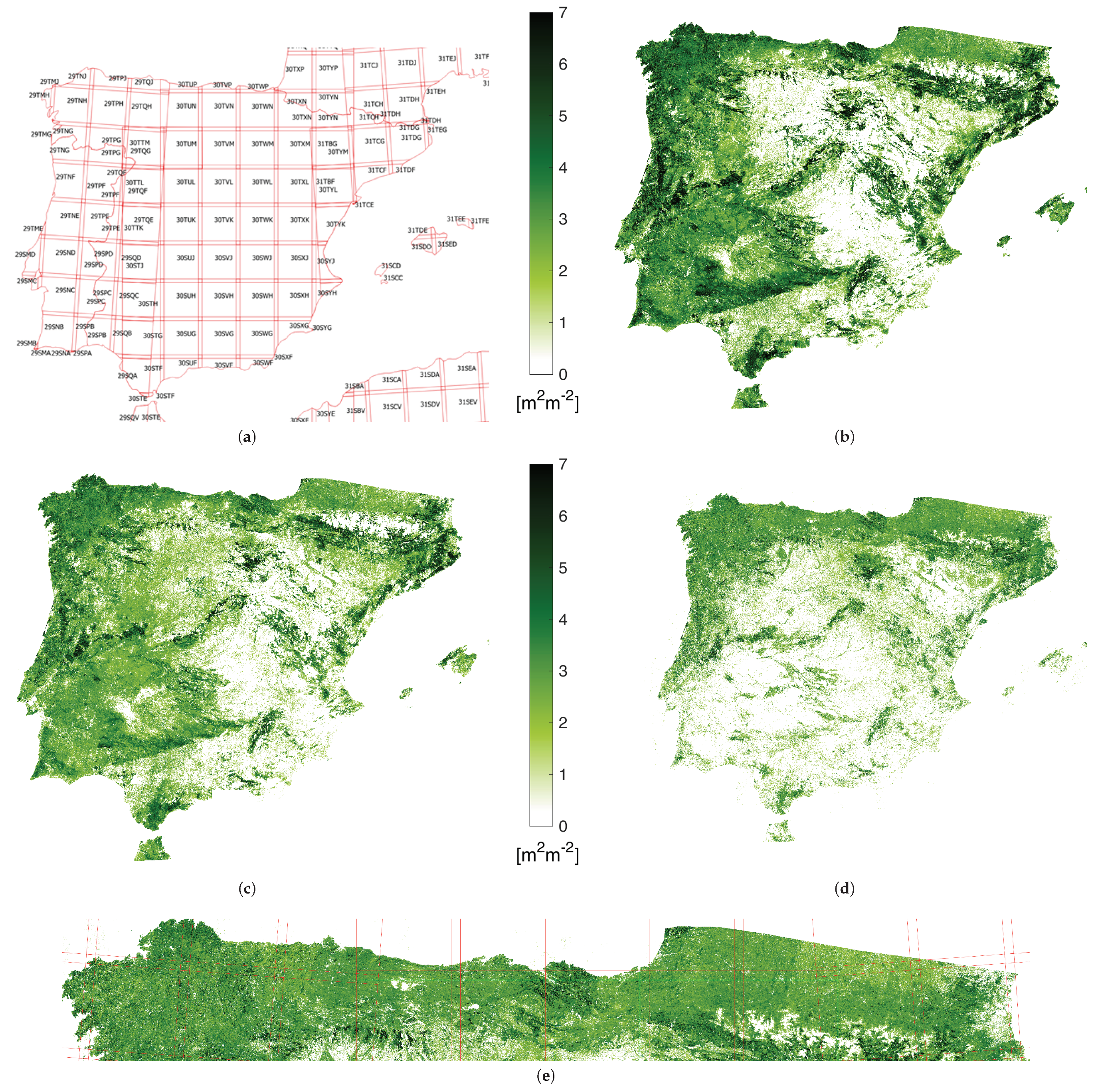
5. Cloud-Free Seamless Mapping of Wide Areas
6. Discussion
7. Conclusions
Supplementary Materials
Author Contributions
Funding
Institutional Review Board Statement
Informed Consent Statement
Acknowledgments
Conflicts of Interest
References
- Weiss, M.; Jacob, F.; Duveiller, G. Remote sensing for agricultural applications: A meta-review. Remote Sens. Environ. 2020, 236, 111402. [Google Scholar] [CrossRef]
- Malenovskỳ, Z.; Homolová, L.; Lukeš, P.; Buddenbaum, H.; Verrelst, J.; Alonso, L.; Schaepman, M.E.; Lauret, N.; Gastellu-Etchegorry, J.P. Variability and uncertainty challenges in scaling imaging spectroscopy retrievals and validations from leaves up to vegetation canopies. Surv. Geophys. 2019, 40, 631–656. [Google Scholar] [CrossRef]
- Verrelst, J.; Rivera, J.P.; Veroustraete, F.; Muñoz-Marí, J.; Clevers, J.G.; Camps-Valls, G.; Moreno, J. Experimental Sentinel-2 LAI estimation using parametric, non-parametric and physical retrieval methods—A comparison. ISPRS J. Photogramm. Remote Sens. 2015, 108, 260–272. [Google Scholar] [CrossRef]
- Verrelst, J.; Malenovskỳ, Z.; Van der Tol, C.; Camps-Valls, G.; Gastellu-Etchegorry, J.P.; Lewis, P.; North, P.; Moreno, J. Quantifying vegetation biophysical variables from imaging spectroscopy data: A review on retrieval methods. Surv. Geophys. 2019, 40, 589–629. [Google Scholar] [CrossRef]
- Baret, F.; Weiss, M.; Lacaze, R.; Camacho, F.; Makhmara, H.; Pacholcyzk, P.; Smets, B. GEOV1: LAI and FAPAR essential climate variables and FCOVER global time series capitalizing over existing products. Part1: Principles of development and production. Remote Sens. Environ. 2013, 137, 299–309. [Google Scholar] [CrossRef]
- Weiss, M.; Baret, F.; Myneni, R.; Pragnère, A.; Knyazikhin, Y. Investigation of a model inversion technique to estimate canopy biophysical variables from spectral and directional reflectance data. Agronomie 2000, 20, 3–22. [Google Scholar] [CrossRef]
- Combal, B.; Baret, F.; Weiss, M. Improving canopy variables estimation from remote sensing data by exploiting ancillary information. Case study on sugar beet canopies. Agronomie 2002, 22, 205–215. [Google Scholar] [CrossRef]
- Verrelst, J.; Muñoz, J.; Alonso, L.; Delegido, J.; Rivera, J.; Camps-Valls, G.; Moreno, J. Machine learning regression algorithms for biophysical parameter retrieval: Opportunities for Sentinel-2 and -3. Remote Sens. Environ. 2012, 118, 127–139. [Google Scholar] [CrossRef]
- Upreti, D.; Huang, W.; Kong, W.; Pascucci, S.; Pignatti, S.; Zhou, X.; Ye, H.; Casa, R. A Comparison of Hybrid Machine Learning Algorithms for the Retrieval of Wheat Biophysical Variables from Sentinel-2. Remote Sens. 2019, 11, 481. [Google Scholar] [CrossRef]
- Verrelst, J.; Camps-Valls, G.; Munoz-Marí, J.; Rivera, J.P.; Veroustraete, F.; Clevers, J.G.; Moreno, J. Optical remote sensing and the retrieval of terrestrial vegetation bio-geophysical properties—A review. ISPRS J. Photogramm. Remote Sens. 2015, 108, 273–290. [Google Scholar] [CrossRef]
- Suykens, J.; Vandewalle, J. Least squares support vector machine classifiers. Neural Process. Lett. 1999, 9, 293–300. [Google Scholar] [CrossRef]
- Vapnik, V.; Golowich, S.; Smola, A. Support vector method for function approximation, regression estimation, and signal processing. Adv. Neural Inf. Process. Syst. 1997, 9, 281–287. [Google Scholar]
- Rasmussen, C.E.; Williams, C.K.I. Gaussian Processes for Machine Learning; The MIT Press: New York, NY, USA, 2006. [Google Scholar]
- Verrelst, J.; Alonso, L.; Camps-Valls, G.; Delegido, J.; Moreno, J. Retrieval of Vegetation Biophysical Parameters Using Gaussian Process Techniques. IEEE Trans. Geosci. Remote Sens. 2012, 50, 1832–1843. [Google Scholar] [CrossRef]
- Verrelst, J.; Rivera, J.P.; Gitelson, A.; Delegido, J.; Moreno, J.; Camps-Valls, G. Spectral band selection for vegetation properties retrieval using Gaussian processes regression. Int. J. Appl. Earth Obs. Geoinf. 2016, 52, 554–567. [Google Scholar] [CrossRef]
- Verrelst, J.; Rivera, J.; Moreno, J.; Camps-Valls, G. Gaussian processes uncertainty estimates in experimental Sentinel-2 LAI and leaf chlorophyll content retrieval. ISPRS J. Photogramm. Remote Sens. 2013, 86, 157–167. [Google Scholar] [CrossRef]
- Chen, Z.; Wang, B. How priors of initial hyperparameters affect Gaussian process regression models. Neurocomputing 2018, 275, 1702–1710. [Google Scholar] [CrossRef]
- Mateo-Sanchis, A.; Muñoz-Marí, J.; Campos-Taberner, M.; García-Haro, J.; Camps-Valls, G. Gap filling of biophysical parameter time series with multi-output Gaussian Processes. In Proceedings of the IGARSS 2018—2018 IEEE International Geoscience and Remote Sensing Symposium, Valencia, Spain, 22–27 July 2018; pp. 4039–4042. [Google Scholar] [CrossRef]
- Pipia, L.; Muñoz-Marí, J.; Amin, E.; Belda, S.; Camps-Valls, G.; Verrelst, J. Fusing optical and SAR time series for LAI gap filling with multioutput Gaussian processes. Remote Sens. Environ. 2019, 235, 111452. [Google Scholar] [CrossRef]
- Belda, S.; Pipia, L.; Morcillo-Pallarés, P.; Rivera-Caicedo, J.P.; Amin, E.; de Grave, C.; Verrelst, J. DATimeS: A machine learning time series GUI toolbox for gap-filling and vegetation phenology trends detection. Environ. Model. Softw. 2020, 104666. [Google Scholar] [CrossRef]
- Amin, E.; Verrelst, J.; Rivera-Caicedo, J.P.; Pipia, L.; Ruiz-Verdú, A.; Moreno, J. Prototyping Sentinel-2 green LAI and brown LAI products for cropland monitoring. Remote Sens. Environ. 2020, 112168. [Google Scholar] [CrossRef]
- Belda, S.; Pipia, L.; Morcillo-Pallarés, P.; Verrelst, J. Optimizing Gaussian Process Regression for Image Time Series Gap-Filling and Crop Monitoring. Agronomy 2020, 10, 618. [Google Scholar] [CrossRef]
- Tona, C.; Bua, R. Open Source Data Hub System: Free and open framework to enable cooperation to disseminate Earth Observation data and geo-spatial information. In Proceedings of the 20th EGU General Assembly, EGU2018, Vienna, Austria, 8–13 April 2018; Volume 20. [Google Scholar]
- Gorelick, N.; Hancher, M.; Dixon, M.; Ilyushchenko, S.; Thau, D.; Moore, R. Google Earth Engine: Planetary-scale geospatial analysis for everyone. Remote Sens. Environ. 2017, 202, 18–27. [Google Scholar] [CrossRef]
- Kumar, L.; Mutanga, O. Google Earth Engine applications since inception: Usage, trends, and potential. Remote Sens. 2018, 10, 1509. [Google Scholar] [CrossRef]
- Verrelst, J.; Alonso, L.; Rivera Caicedo, J.; Moreno, J.; Camps-Valls, G. Gaussian Process Retrieval of Chlorophyll Content From Imaging Spectroscopy Data. IEEE J. Sel. Top. Appl. Earth Obs. Remote Sens. 2013, 6, 867–874. [Google Scholar] [CrossRef]
- Campos-Taberner, M.; García-Haro, F.J.; Camps-Valls, G.; Grau-Muedra, G.; Nutini, F.; Crema, A.; Boschetti, M. Multitemporal and multiresolution leaf area index retrieval for operational local rice crop monitoring. Remote Sens. Environ. 2016, 187, 102–118. [Google Scholar] [CrossRef]
- Amin, E.; Verrelst, J.; Rivera-Caicedo, J.P.; Pasqualotto, N.; Delegido, J.; Verdú, A.R.; Moreno, J. The Sensagri Sentinel-2 LAI Green and Brown Product: From Algorithm Development Towards Operational Mapping. In Proceedings of the IGARSS 2018—2018 IEEE International Geoscience and Remote Sensing Symposium, Valencia, Spain, 22–27 July 2018; pp. 1822–1825. [Google Scholar]
- Camps-Valls, G.; Jung, M.; Ichii, K.; Papale, D.; Tramontana, G.; Bodesheim, P.; Schwalm, C.; Zscheischler, J.; Mahecha, M.; Reichstein, M. Ranking drivers of global carbon and energy fluxes over land. In Proceedings of the 2015 IEEE International Geoscience and Remote Sensing Symposium (IGARSS), Milan, Italy, 26–31 July 2015; pp. 4416–4419. [Google Scholar]
- Camps-Valls, G.; Verrelst, J.; Muñoz-Marí, J.; Laparra, V.; Mateo-Jiménez, F.; Gómez-Dans, J. A Survey on Gaussian Processes for Earth Observation Data Analysis. IEEE Geosci. Remote Sens. Mag. 2016, 4, 58–78. [Google Scholar] [CrossRef]
- Camps-Valls, G.; Sejdinovic, D.; Runge, J.; Reichstein, M. A Prspective on Gaussian Processes for Earth Observation. Natl. Sci. Rev. 2019. [Google Scholar] [CrossRef]
- Aye, S.; Heyns, P. An integrated Gaussian process regression for prediction of remaining useful life of slow speed bearings based on acoustic emission. Mech. Syst. Signal Process. 2017, 84, 485–498. [Google Scholar] [CrossRef]
- Calandriello, D.; Carratino, L.; Lazaric, A.; Valko, M.; Rosasco, L. Near-linear time Gaussian process optimization with adaptive batching and resparsification. In Proceedings of the 37th International Conference on Machine Learning, Vienna, Austria, 13–18 July 2020; pp. 1295–1305. [Google Scholar]
- Verrelst, J.; Rivera, J.; Alonso, L.; Moreno, J. ARTMO: An Automated Radiative Transfer Models Operator toolbox for automated retrieval of biophysical parameters through model inversion. In Proceedings of the 7th EARSeL Workshop on Imaging Spectrometry, Brno, Czech Republic, 6–8 February 2011. [Google Scholar]
- Blum, M.; Riedmiller, M. Optimization of Gaussian Process Hyperparameters using Rprop. In Proceedings of the 21th European Symposium on Artificial Neural Networks, Computational Intelligence and Machine Learning, Bruges, Belgium, 24–26 April 2013. [Google Scholar]
- Jonckheere, I.; Fleck, S.; Nackaerts, K.; Muys, B.; Coppin, P.; Weiss, M.; Baret, F. Review of methods for in situ leaf area index determination Part I. Theories, sensors and hemispherical photography. Agric. For. Meteorol. 2004, 121, 19–35. [Google Scholar] [CrossRef]
- Boegh, E.; Søgaard, H.; Broge, N.; Hasager, C.; Jensen, N.; Schelde, K.; Thomsen, A. Airborne multispectral data for quantifying leaf area index, nitrogen concentration, and photosynthetic efficiency in agriculture. Remote Sens. Environ. 2002, 81, 179–193. [Google Scholar] [CrossRef]
- Duveiller, G.; Baret, F.; Defourny, P. Remotely sensed green area index for winter wheat crop monitoring: 10-Year assessment at regional scale over a fragmented landscape. Agric. For. Meteorol. 2012, 166, 156–168. [Google Scholar] [CrossRef]
- Drusch, M.; Del Bello, U.; Carlier, S.; Colin, O.; Fernandez, V.; Gascon, F.; Hoersch, B.; Isola, C.; Laberinti, P.; Martimort, P.; et al. Sentinel-2: ESA’s Optical High-Resolution Mission for GMES Operational Services. Remote Sens. Environ. 2012, 120, 25–36. [Google Scholar] [CrossRef]
- Verrelst, J.; Dethier, S.; Rivera, J.P.; Munoz-Mari, J.; Camps-Valls, G.; Moreno, J. Active Learning Methods for Efficient Hybrid Biophysical Variable Retrieval. IEEE Geosci. Remote Sens. Lett. 2016, 13, 1012–1016. [Google Scholar] [CrossRef]
- Verrelst, J.; Berger, K.; Rivera-Caicedo, J.P. Intelligent sampling for vegetation nitrogen mapping based on hybrid machine learning algorithms. IEEE Geosci. Remote Sens. Lett. 2020. [Google Scholar] [CrossRef]
- Rivera-Caicedo, J.P.; Verrelst, J.; Muñoz-Marí, J.; Camps-Valls, G.; Moreno, J. Hyperspectral dimensionality reduction for biophysical variable statistical retrieval. ISPRS J. Photogramm. Remote Sens. 2017, 132, 88–101. [Google Scholar] [CrossRef]
- D’Odorico, P.; Gonsamo, A.; Gough, C.M.; Bohrer, G.; Morison, J.; Wilkinson, M.; Hanson, P.J.; Gianelle, D.; Fuentes, J.D.; Buchmann, N. The match and mismatch between photosynthesis and land surface phenology of deciduous forests. Agric. For. Meteorol. 2015, 214–215, 25–38. [Google Scholar] [CrossRef]
- Kuenzer, C.; Dech, S.; Wagner, W. Remote Sensing Time Series Revealing Land Surface Dynamics. Remote Sens. Time Ser. 2015, 22. [Google Scholar] [CrossRef]
- Weiss, D.J.; Atkinson, P.M.; Bhatt, S.; Mappin, B.; Hay, S.I.; Gething, P.W. An effective approach for gap-filling continental scale remotely sensed time-series. ISPRS J. Photogramm. Remote Sens. 2014, 98, 106–118. [Google Scholar] [CrossRef]
- Mariethoz, G.; McCabe, M.; Renard, P. Spatiotemporal reconstruction of gaps in multivariate fields using the direct sampling approach. Water Resour. Res. 2012, 48. [Google Scholar] [CrossRef]
- Chen, J.; Boccelli, D.L. Real-time forecasting and visualization toolkit for multi-seasonal time series. Environ. Model. Softw. 2018, 105, 244–256. [Google Scholar] [CrossRef]
- Jönsson, P.; Cai, Z.; Melaas, E.; Friedl, M.A.; Eklundh, L. A Method for Robust Estimation of Vegetation Seasonality from Landsat and Sentinel-2 Time Series Data. Remote Sens. 2018, 10, 635. [Google Scholar] [CrossRef]
- Camps-Valls, G.; Martino, L.; Svendsen, D.H.; Campos-Taberner, M.; Muñoz-Marí, J.; Laparra, V.; Luengo, D.; García-Haro, F.J. Physics-aware Gaussian processes in remote sensing. Appl. Soft Comput. 2018, 68, 69–82. [Google Scholar] [CrossRef]
- Hensman, J.; Fusi, N.; Lawrence, N.D. Gaussian Processes for Big Data. arXiv 2013, arXiv:1309.6835. [Google Scholar]
- Moore, C.; Chua, A.; Berry, C.; Gair, J. Fast methods for training gaussian processes on large datasets. R. Soc. Open Sci. 2016, 3. [Google Scholar] [CrossRef] [PubMed]
- Klein, T.; Nilsson, M.; Persson, A.; Håkansson, B. From Open Data to Open Analyses—New Opportunities for Environmental Applications? Environments 2017, 4, 32. [Google Scholar] [CrossRef]
- Chen, B.; Xiao, X.; Li, X.; Pan, L.; Doughty, R.; Ma, J.; Dong, J.; Qin, Y.; Zhao, B.; Wu, Z.; et al. A mangrove forest map of China in 2015: Analysis of time series Landsat 7/8 and Sentinel-1A imagery in Google Earth Engine cloud computing platform. ISPRS J. Photogramm. Remote Sens. 2017, 131, 104–120. [Google Scholar] [CrossRef]
- Deines, J.M.; Kendall, A.D.; Hyndman, D.W. Annual irrigation dynamics in the US Northern High Plains derived from Landsat satellite data. Geophys. Res. Lett. 2017, 44, 9350–9360. [Google Scholar] [CrossRef]
- ESA. ESA Scientific Hub. Available online: https://scihub.copernicus.eu/dhus/#/home (accessed on 10 January 2021).
- Louis, J.; Debaecker, V.; Pflug, B.; Main-Knorn, M.; Bieniarz, J.; Mueller-Wilm, U.; Cadau, E.; Gascon, F. Sentinel-2 Sen2Cor: L2A processor for users. In Proceedings of the Living Planet Symposium 2016, Prague, Czech Republic, 9–13 May 2016; pp. 1–8. [Google Scholar]
- Google Earth Engine Debugging Guide. Available online: https://developers.google.com/earth-engine/guides (accessed on 10 January 2021).
- AEMET, I. Atlas climático ibérico/Iberian climate atlas. In Agencia Estatal de Meteorología, Ministerio de Medio Ambiente y Rural y Marino; Instituto de Meteorologia de Portugal: Madrid, Spain, 2011. [Google Scholar]
- Azorin-Molina, C.; Vicente-Serrano, S.M.; Chen, D.; Connell, B.H.; Domínguez-Durán, M.Á.; Revuelto, J.; López-Moreno, J.I. AVHRR warm-season cloud climatologies under various synoptic regimes across the Iberian Peninsula and the Balearic Islands. Int. J. Climatol. 2015, 35, 1984–2002. [Google Scholar] [CrossRef]
- Li, H.; Wan, W.; Fang, Y.; Zhu, S.; Chen, X.; Liu, B.; Hong, Y. A Google Earth Engine-enabled software for efficiently generating high-quality user-ready Landsat mosaic images. Environ. Model. Softw. 2019, 112, 16–22. [Google Scholar] [CrossRef]
- Tamiminia, H.; Salehi, B.; Mahdianpari, M.; Quackenbush, L.; Adeli, S.; Brisco, B. Google Earth Engine for geo-big data applications: A meta-analysis and systematic review. ISPRS J. Photogramm. Remote Sens. 2020, 164, 152–170. [Google Scholar] [CrossRef]
- Wu, Q.; Lane, C.R.; Li, X.; Zhao, K.; Zhou, Y.; Clinton, N.; DeVries, B.; Golden, H.E.; Lang, M.W. Integrating LiDAR data and multi-temporal aerial imagery to map wetland inundation dynamics using Google Earth Engine. Remote Sens. Environ. 2019, 228, 1–13. [Google Scholar] [CrossRef]
- Wu, Q. Geemap: A Python package for interactive mapping with Google Earth Engine. J. Open Source Softw. 2020, 5, 2305. [Google Scholar] [CrossRef]
- Kennedy, R.E.; Yang, Z.; Gorelick, N.; Braaten, J.; Cavalcante, L.; Cohen, W.B.; Healey, S. Implementation of the LandTrendr algorithm on google earth engine. Remote Sens. 2018, 10, 691. [Google Scholar] [CrossRef]
- Google Earth Engine Developers’ Forum Guide. Available online: https://groups.google.com/g/google-earth-engine-developers?pli=1 (accessed on 10 January 2021).
- Wu, Q. Earth Engine Python Tutorials. Available online: https://www.youtube.com/c/QiushengWu/featured/ (accessed on 10 January 2021).
- Gisandbeers. Scripts for Google Earth Engine. Available online: http://www.gisandbeers.com/scripts-para-google-earth-engine/ (accessed on 10 January 2021).
- Lakshminarayanan, B.; Pritzel, A.; Blundell, C. Simple and scalable predictive uncertainty estimation using deep ensembles. Adv. Neural Inf. Process. Syst. 2017, 30, 6402–6413. [Google Scholar]
- Novak, R.; Xiao, L.; Hron, J.; Lee, J.; Alemi, A.A.; Sohl-Dickstein, J.; Schoenholz, S.S. Neural tangents: Fast and easy infinite neural networks in python. arXiv 2019, arXiv:1912.02803. [Google Scholar]
- Lee, J.; Bahri, Y.; Novak, R.; Schoenholz, S.S.; Pennington, J.; Sohl-Dickstein, J. Deep neural networks as gaussian processes. arXiv 2017, arXiv:1711.00165. [Google Scholar]
- Novak, R.; Xiao, L.; Lee, J.; Bahri, Y.; Yang, G.; Hron, J.; Abolafia, D.A.; Pennington, J.; Sohl-Dickstein, J. Bayesian deep convolutional networks with many channels are gaussian processes. arXiv 2018, arXiv:1810.05148. [Google Scholar]
- Sobrino, J.; Julien, Y. Global trends in NDVI-derived parameters obtained from GIMMS data. Int. J. Remote Sens. 2011, 32, 4267–4279. [Google Scholar] [CrossRef]
- Richardson, A.; Keenan, T.; Migliavacca, M.; Ryu, Y.; Sonnentag, O.; Toomey, M. Climate change, phenology, and phenological control of vegetation feedbacks to the climate system. Agric. For. Meteorol. 2013, 169, 156–173. [Google Scholar] [CrossRef]
- Atzberger, C. Advances in remote sensing of agriculture: Context description, existing operational monitoring systems and major information needs. Remote Sens. 2013, 5, 949–981. [Google Scholar] [CrossRef]
- Sobrino, J.A.; Julien, Y.; Sòria, G. Phenology Estimation From Meteosat Second Generation Data. IEEE J. Sel. Top. Appl. Earth Obs. Remote Sens. 2013, 6, 1653–1659. [Google Scholar] [CrossRef]
- Hill, M.J.; Donald, G.E. Estimating spatio-temporal patterns of agricultural productivity in fragmented landscapes using AVHRR NDVI time series. Remote Sens. Environ. 2003, 84, 367–384. [Google Scholar] [CrossRef]
- Overpeck, J.T.; Rind, D.; Goldberg, R. Climate-induced changes in forest disturbance and vegetation. Nature 1990, 343, 51–53. [Google Scholar] [CrossRef]
- Frantz, D.; Röder, A.; Udelhoven, T.; Schmidt, M. Forest disturbance mapping using dense synthetic landsat/MODIS time-series and permutation-based disturbance index detection. Remote Sens. 2016, 8, 277. [Google Scholar] [CrossRef]
- Masek, J.G.; Huang, C.; Wolfe, R.; Cohen, W.; Hall, F.; Kutler, J.; Nelson, P. North American forest disturbance mapped from a decadal Landsat record. Remote Sens. Environ. 2008, 112, 2914–2926. [Google Scholar] [CrossRef]
- Zhao, K.; Wulder, M.A.; Hu, T.; Bright, R.; Wu, Q.; Qin, H.; Li, Y.; Toman, E.; Mallick, B.; Zhang, X.; et al. Detecting change-point, trend, and seasonality in satellite time series data to track abrupt changes and nonlinear dynamics: A Bayesian ensemble algorithm. Remote Sens. Environ. 2019, 232, 111181. [Google Scholar] [CrossRef]
- Lastovicka, J.; Svec, P.; Paluba, D.; Kobliuk, N.; Svoboda, J.; Hladky, R.; Stych, P. Sentinel-2 Data in an Evaluation of the Impact of the Disturbances on Forest Vegetation. Remote Sens. 2020, 12, 1914. [Google Scholar] [CrossRef]
- Verbesselt, J.; Hyndman, R.; Newnham, G.; Culvenor, D. Detecting Trend and Seasonal Changes in Satellite Image Time Series. Remote Sens. Environ. 2010, 114, 106–115. [Google Scholar] [CrossRef]
- Zhang, X.; Zhang, Q. Monitoring interannual variation in global crop yield using long-term AVHRR and MODIS observations. ISPRS J. Photogramm. Remote Sens. 2016, 114, 191–205. [Google Scholar] [CrossRef]
- Baker, N. Chlorophyll fluorescence: A probe of photosynthesis in vivo. Annu. Rev. Plant Biol. 2008, 59, 89–113. [Google Scholar] [CrossRef]
- Mohammed, G.H.; Colombo, R.; Middleton, E.M.; Rascher, U.; van der Tol, C.; Nedbal, L.; Goulas, Y.; Pérez-Priego, O.; Damm, A.; Meroni, M.; et al. Remote sensing of solar-induced chlorophyll fluorescence (SIF) in vegetation: 50 years of progress. Remote Sens. Environ. 2019, 231, 111177. [Google Scholar] [CrossRef]


| Location | Period | #Points | Range | Instrument | Vegetation Type | Spectral Data |
|---|---|---|---|---|---|---|
| Barrax, Spain | 3 July | 102 | 0.4–6.2 | LAI-2000 | Alfalfa, corn, garlic, onion, potato, sugar beet, wheat | HyMap |
| Valencia, Spain | May–17 November | 34 | 0.41–5.41 | LAI-2200 | Alfalfa, artichoke, lettuce, onion, potato | S2 |
| Biely Kríž, Czech Republic | 16 August | 7 | 5.3–9.3 | LAI-2200 | Spruce forest | S2 |
| Foggia, Italy | 17 March | 6 | 3.08–4.23 | LAI-2200 | Wheat | S2 |
| Poznań, Poland | 17 July | 6 | 2.69–4.2 | LAI-2200 | Maize, triticale, wheat | S2 |
| Kiev Oblast, Ukraine | 18 June | 3 | 0.27–0.56 | DHP | Maize, soybean | S2 |
| Toulouse, France | 18 August | 1 | 1.77 | DHP | Maize | S2 |
| Location | Period | #Points | Range | Instrument | Vegetation Type | Spectral Data |
|---|---|---|---|---|---|---|
| Toulouse, France | Nov17/Mar-May-Jul-Aug 18 | 52 | 0.03–3.84 | DHP | Maize, soybean, sunflower | S2 |
| Poznań, Poland | Apr-Jun-Aug 18 | 50 | 0.96–4.23 | LAI-2200 | Beetroot, maize, triticale, wheat | S2 |
| Kiev Oblast, Ukraine | May-Jun-Aug 18 | 40 | 0.04–4.81 | DHP | Maize, soybean, sunflower, wheat | S2 |
| Wheat | Corn | Barley | Sunflower | Rape | Pea | Alfalfa | Beet | Potato | Global | |
|---|---|---|---|---|---|---|---|---|---|---|
| 32.6018 | 41.0726 | 36.0351 | 23.0815 | 35.0548 | 23.9367 | 29.8602 | 47.3544 | 25.5081 | 32.7282 | |
| 0.8776 | 1.0018 | 0.8395 | 0.5670 | 1.2058 | 0.8415 | 0.6465 | 1.1465 | 1.1870 | 0.9237 | |
| 0.3377 | 0.4395 | 0.2833 | 0.2355 | 0.5085 | 0.2778 | 0.4028 | 0.3794 | 0.3620 | 0.3585 |
| Crop Type | Per-Pixel Hyperpar. | Averaged Hyperparameters | Variance | |||||||||
|---|---|---|---|---|---|---|---|---|---|---|---|---|
| Wheat | Corn | Barley | Sunflower | Rape | Pea | Alfalfa | Beet | Potato | Global | |||
| Wheat | 9.064 | 10.078 | 10.845 | 10.240 | 9.072 | 10.372 | 8.851 | 10.519 | 10.996 | 8.995 | 10.097 | 0.787 |
| Corn | 10.660 | 10.794 | 11.614 | 10.952 | 9.821 | 11.100 | 9.675 | 11.174 | 11.752 | 9.812 | 10.813 | 0.708 |
| Barley | 8.206 | 8.593 | 9.282 | 8.707 | 7.932 | 8.834 | 7.739 | 9.058 | 9.435 | 7.826 | 8.608 | 0.580 |
| Sunflower | 8.455 | 11.238 | 12.366 | 11.474 | 9.928 | 11.642 | 9.752 | 11.646 | 12.633 | 9.929 | 11.263 | 1.265 |
| Rape | 10.222 | 10.798 | 11.483 | 10.950 | 9.576 | 11.070 | 9.351 | 11.207 | 11.598 | 9.573 | 10.816 | 0.799 |
| Pea | 7.634 | 10.017 | 11.601 | 10.314 | 8.719 | 10.557 | 8.485 | 10.671 | 12.026 | 8.624 | 10.050 | 1.371 |
| Alfalfa | 11.833 | 14.001 | 14.999 | 14.222 | 12.659 | 14.368 | 12.496 | 14.360 | 15.210 | 12.734 | 14.024 | 1.108 |
| Beet | 8.975 | 8.975 | 9.629 | 9.083 | 8.207 | 9.223 | 8.054 | 9.389 | 9.714 | 8.149 | 8.991 | 0.577 |
| Potato | 7.477 | 9.456 | 10.566 | 9.647 | 8.311 | 9.848 | 8.130 | 9.993 | 10.769 | 8.262 | 9.481 | 1.070 |
| (var) calculate_LAI_GREEN = function(image){ |
| (var) = image.multiply(D).toArray().toArray(1); |
| (var) = image.toArray().toArray(1); |
| (var) Term1 = .matrixTranspose().matrixMultiply().arrayProject([0]).multiply(−0.5).exp().multiply() |
| (var) PtTDX = ee.Image(X).matrixMultiply().arrayProject([0]).arrayFlatten([TS_ID]); |
| (var) = PtTDX.subtract(.multiply(0.5)).exp().toArray() |
| (var) f() = .arrayDotProduct(.toArray()).multiply(Term1).toArray(1).arrayProject([0]).arrayFlatten([[‘LAIG’]]); |
| return image.select(‘LAIG’)} |
| (var) NLAIG.size(); |
| (var) .multiply(0).add(1.0); |
| (var) .multiply(0).add(1.0); |
| (var) I = ee.Image(ee.Array.identity(N)); |
| (var) prod = .matrixMultiply(1.matrixTranspose()); |
| (var) K.subtract(prod.matrixTranspose()).pow(2).multiply().multiply().exp().multiply(); |
| (var) L = I.multiply().add().matrixCholeskyDecomposition(); |
| (var) = L.matrixInverse().matrixMultiply(.toBands().unmask().toArray().toArray(1)); |
| (var) = L.matrixTranspose().matrixInverse().matrixMultiply(); |
| (var) .matrixMultiply(.matrixTranspose()); |
| (var) = .matrixMultiply(matrixTranspose()).matrixTranspose(); |
| (var) = .subtract().pow(2).multiply().multiply().exp().multiply(); |
| (var) ) = .matrixMultiply().arrayProject([0]).arrayFlatten([[‘LAIG’]]); |
Publisher’s Note: MDPI stays neutral with regard to jurisdictional claims in published maps and institutional affiliations. |
© 2021 by the authors. Licensee MDPI, Basel, Switzerland. This article is an open access article distributed under the terms and conditions of the Creative Commons Attribution (CC BY) license (http://creativecommons.org/licenses/by/4.0/).
Share and Cite
Pipia, L.; Amin, E.; Belda, S.; Salinero-Delgado, M.; Verrelst, J. Green LAI Mapping and Cloud Gap-Filling Using Gaussian Process Regression in Google Earth Engine. Remote Sens. 2021, 13, 403. https://doi.org/10.3390/rs13030403
Pipia L, Amin E, Belda S, Salinero-Delgado M, Verrelst J. Green LAI Mapping and Cloud Gap-Filling Using Gaussian Process Regression in Google Earth Engine. Remote Sensing. 2021; 13(3):403. https://doi.org/10.3390/rs13030403
Chicago/Turabian StylePipia, Luca, Eatidal Amin, Santiago Belda, Matías Salinero-Delgado, and Jochem Verrelst. 2021. "Green LAI Mapping and Cloud Gap-Filling Using Gaussian Process Regression in Google Earth Engine" Remote Sensing 13, no. 3: 403. https://doi.org/10.3390/rs13030403
APA StylePipia, L., Amin, E., Belda, S., Salinero-Delgado, M., & Verrelst, J. (2021). Green LAI Mapping and Cloud Gap-Filling Using Gaussian Process Regression in Google Earth Engine. Remote Sensing, 13(3), 403. https://doi.org/10.3390/rs13030403