Article

Incident Angle Dependence of Sentinel-1 Texture Features for Sea Ice Classification

by
Johannes Lohse
1,*,
Anthony P. Doulgeris
1 and
Wolfgang Dierking
1,2
1
Department of Physics and Technology, UiT The Arctic University of Norway, 9019 Tromsø, Norway
2
Alfred Wegener Institute, Helmholtz Center for Polar and Marine Research, Bussestr. 24, 27570 Bremerhaven, Germany
*
Author to whom correspondence should be addressed.
Remote Sens. 2021, 13(4), 552; https://doi.org/10.3390/rs13040552
Submission received: 24 December 2020 / Revised: 22 January 2021 / Accepted: 1 February 2021 / Published: 4 February 2021
(This article belongs to the Special Issue Remote Sensing of Sea Ice and Icebergs)

Abstract

:
Robust and reliable classification of sea ice types in synthetic aperture radar (SAR) images is needed for various operational and environmental applications. Previous studies have investigated the class-dependent decrease in SAR backscatter intensity with incident angle (IA); others have shown the potential of textural information to improve automated image classification. In this work, we investigate the inclusion of Sentinel-1 (S1) texture features into a Bayesian classifier that accounts for linear per-class variation of its features with IA. We use the S1 extra-wide swath (EW) product in ground-range detected format at medium resolution (GRDM), and we compute seven grey level co-occurrence matrix (GLCM) texture features from the HH and the HV backscatter intensity in the linear and logarithmic domain. While GLCM texture features obtained in the linear domain vary significantly with IA, the features computed from the logarithmic intensity do not depend on IA or reveal only a weak, approximately linear dependency. They can therefore be directly included in the IA-sensitive classifier that assumes a linear variation. The different number of looks in the first sub-swath (EW1) of the product causes a distinct offset in texture at the sub-swath boundary between EW1 and the second sub-swath (EW2). This offset must be considered when using texture in classification; we demonstrate a manual correction for the example of GLCM contrast. Based on the Jeffries–Matusita distance between class histograms, we perform a separability analysis for 57 different GLCM parameter settings. We select a suitable combination of features for the ice classes in our data set and classify several test images using a combination of intensity and texture features. We compare the results to a classifier using only intensity. Particular improvements are achieved for the generalized separation of ice and water, as well as the classification of young ice and multi-year ice.

Graphical Abstract

1. Introduction

Synthetic aperture radar (SAR) is a primary tool for monitoring of sea ice conditions in the polar regions [1,2,3]. A radar system is an active device that both transmits and receives electromagnetic radiation in the microwave region, and is thus independent of sunlight and cloud conditions. The resulting continuous imaging capability of the SAR is important for operational ice services worldwide [3,4]. The analysis and interpretation of the SAR images and the production of ice charts is at present carried out manually and therefore subject to the expertise of the individual ice analyst [5,6]. Furthermore, while timeliness of ice charts is a critical requirement, the manual image analysis is a time-consuming process [7]. In combination with an increasing volume of available SAR imagery, this underlines the need for automated or computer-assisted classification of sea ice. The backscatter signature of sea ice in radar images, however, depends on a variety of different factors, including sea ice, environmental, and radar parameters [8,9]. Despite multiple efforts and various approaches, robust and automated classification of ice types therefore remains a challenging task [3].
The important radar parameters that influence the signal include radar frequency, polarization, and incident angle (IA) [9]. While frequency and polarization are fixed for a given sensor and operation mode, IA varies across the image. The backscatter intensity (also referred to as image brightness or tone) from a homogeneous surface varies with IA and decreases across a SAR image from near-range (low IA) to far-range (high IA). In the logarithmic domain, i.e., with the intensity given in dB, the decrease is approximately linear with a constant slope per surface class [10,11,12,13]. Despite many studies showing that the rate of decrease differs between different surface types, most classification approaches apply a global IA correction during pre-processing, using a constant slope for the entire SAR image [14,15,16,17,18]. Although such approaches can achieve good results, they neglect the known physical differences in backscatter behavior with IA for different surface types. Lohse et al. [19] recently introduced a method to directly incorporate the class-dependent effect of IA into a supervised algorithm. The method is based on a Bayesian classifier (i.e., it maximizes probabilities) with multi-variate Gaussian probability density functions (PDFs), where the constant mean value is replaced with a linearly varying mean value. The linear slopes are class-dependent and thus directly included in the classifier. Since it is based on underlying Gaussian PDFs and accounts for a per-class IA effect, the classification method is referred to as the GIA (Gaussian incident angle) classifier. The approach achieves improved classification results compared to intensity-based methods with a global IA correction. However, ambiguities in backscatter intensity remain for individual classes at some IA ranges [19]. In particular, changes in the sea surface roughness (the sea surface state), caused for example by varying wind conditions, ocean currents, or natural and oil slicks, can complicate the reliable classification of open water (OW).
Previous studies have shown that in many cases textural information can help to resolve ambiguities in sea ice classification, both for the binary problem of ice-water classification and for the multi-class separation of different ice types [18,20,21,22,23,24,25,26,27]. Texture generally refers to the local spatial variation of tone or brightness within an image at a given scale [28]. While many different ways of extracting texture features exist [24], the most common texture features used for sea ice classification are based on the grey level co-occurrence matrix (GLCM) [28]. A straightforward way to directly utilize information from the GLCM in a pixel-based classifier is to extract scalar features from the matrix. Such GLCM-based texture features have been used in a variety of studies and algorithms and improved overall classification accuracy (CA) of OW areas vs. sea ice [14,18,21,22,23,24,25,27,29]. Texture extraction, and in particular computation of the GLCM, requires several input parameters such as window size, quantization levels, displacement distance, and displacement direction (see Section 3 for details). Many of these parameters have been investigated in previous studies. The optimal choice, however, differs between studies (Table 1) and depends on class definitions and data properties. To our best knowledge, a systematic investigation of the dependence of common GLCM texture features on IA for different classes has not been performed prior to this study. All approaches presented in the literature that use the GLCM for the analysis of sea ice imagery either apply a global IA correction or no correction.
In this study, we therefore investigate the per-class IA dependence of different texture features. We do so with the intention of incorporating texture directly into the GIA classifier, which accounts for per-class IA effects. The main prerequisite for this incorporation is that there must be a clearly defined relationship between texture parameters and IA. Ideally, for the linear GIA, this relationship should be constant or linear, and the distribution of the individual features around the linear function can be approximated as Gaussian. These ideal conditions allow for the direct use of the texture features in the existing algorithm, while a more complicated IA relationship or a clearly non-Gaussian distribution would require changing the underlying model of the GIA classifier. After we confirm that common texture features fulfill these conditions, we select a useful set of features and demonstrate the benefits of including them in the classification process.
This paper is organized as follows. Section 2 gives an overview of the data set, including the standard pre-processing steps that were applied. The outline of the investigations in this study is presented in Section 3, followed by a detailed description of the computation and selection of the texture features as well as the tested parameter settings. Section 4 presents the results of these investigations. We discuss our findings in Section 5, pointing out implications and limitations for the usage of texture in sea ice type classification from SAR data, and in particular in the GIA classifier. In Section 6, we summarize the main findings and conclusions.

2. Data

2.1. Sentinel-1 Data

All SAR imagery in this study is Sentinel-1 (S1) data acquired in extra-wide swath (EW) operation mode [30]. S1 operates at C-band (5.4 GHz) providing either single- or dual-polarization data. As part of the European Copernicus Earth observation program, all S1 data are freely available (e.g., through the Copernicus Open Access Hub). The data used in this study are acquired at dual-polarization (HH and HV) and downloaded in ground-range detected format at medium resolution (GRDM). The EW GRDM product comes at a pixel spacing of 40 × 40 m with an actual spatial resolution of approximately 93 × 87 m; its values are multi-looked intensities with 18 looks in the first sub-swath EW1 and 12 looks in the remaining sub-swaths EW2 to EW5. As standard pre-processing, we apply the thermal noise correction implemented in ESA’s Sentinel Application Platform (SNAP) and calibrate the data to obtain the normalized radar cross-section σ 0 . All processing is performed in the ground-range detected image geometry.

2.2. Training and Validation Data

We use the training and validation data set introduced by Lohse et al. [19] in 2020. This data set is based on the visual inspection and expert analysis of overlapping SAR (S1) and optical remote sensing data acquired during winter conditions between 2015 and 2019. The main identified classes in the data set are open water (OW), leads with OW or newly formed ice (NFI), brash or pancake ice, young ice (YI), level first-year ice (LFYI), deformed first-year ice (DFYI), and multi-year ice (MYI). A detailed description of the data set, image locations and acquisition times, and the selection of classes and training polygons is given in Lohse et al. [19]. For parts of this study, we have added new images and test polygons to the existing data set. Generally, the training data for individual classes used in this study are collected from a large number of scenes. In some cases we show training data from a single image for a particular class. The image IDs (product unique IDs) are given in the respective subsections of this article.

3. Method

3.1. Domain-Dependent Texture Extraction and Calculation of Separability

After pre-processing, we extract various texture features from both the HH and the HV channel of the S1 images. Initially, we compute all texture features from both the backscatter intensity in the linear domain (normalized radar cross-section σ 0 ) and the backscatter intensity in the logarithmic domain. In the logarithmic domain, the intensities are given in decibels (dB):
HH dB = 10 · log 10 ( σ H H 0 ) HV dB = 10 · log 10 ( σ H V 0 )
The relationship of intensity with IA is approximately exponential in the linear domain, and thus in turn approximately linear in the logarithmic domain (Figure 1). These differences in IA dependence, in combination with the change of variance with IA in the linear domain, are expected to translate into differences in IA dependence of the texture features extracted from the respective intensity domains.
The initial extraction of texture from both linear and logarithmic intensity allows us to find the preferred domain to compute the texture features. For the preferred domain, we test a variety of parameter settings (see Section 3.2.1 and Section 3.2.2 for details), and investigate the variation of the extracted features with IA for these different settings. We adjust the borders of the training regions according to the size of the texture windows, such that little or no mixing of ice classes occurs within the texture windows. We then use the Jeffries–Matusita (JM) distance [31] to evaluate all features and parameter settings in terms of class separability for various two-class cases.
The JM distance is an established separability measure between class distributions that returns values between zero (no separability) and two (perfect separability). It is given by
J M = 2 ( 1 e D B ) ,
where D B is the Bhattacharrya distance according to
D B = 1 8 ( μ 1 μ 2 ) T Σ 1 ( μ 1 μ 2 ) + 1 2 ln det Σ det Σ 1 det Σ 2
Features with a JM value above one are commonly considered useful for classification [31].
On the basis of this evaluation, we finally select a suitable feature set and demonstrate the benefits of incorporating textural information into the GIA classifier. In particular, we present examples for the classification of sea ice against OW, as well as YI against MYI, and compare against results obtained from a classifier based on intensities only.

3.2. Calculation of Texture Features

Since many previous studies suggest that the GLCM provides a useful method to generate texture features that can improve sea ice classification results [24,26], we focus on this method (Section 3.2.1). However, calculation of the GLCM is computationally expensive and time-consuming, which can impede its use in operational applications. As an example for a simpler and more easily calculated texture feature, we therefore also extract the variance (Section 3.2.2) and assess its usability compared to the GLCM features.

3.2.1. GLCM Texture Features

The GLCM provides a second-order statistic for extraction of texture features [25,28]. It calculates the probability of a pixel with grey level value i occurring at a certain distance and angle from another pixel with grey level j within a given window. The key parameters that must be set are the window size w for which to calculate the GLCM, the co-occurrence distance d, the displacement angle α , and the number of grey level quantization intervals k. Algebraically, the GLCM can be expressed as
S w , d , α , k ( i , j ) = P w , d , α , k ( i , j ) i = 1 k j = 1 k P w , d , α , k ( i , j )
where S w , d , α , k is an element of the GLCM for a given window size, direction, co-occurrence distance, and grey level quantization; P w , d , α , k is the frequency of occurrence of grey levels i and j; and k is the number of quantized grey levels. The size of the GLCM depends on the number of grey levels. In order to neglect effects from ice floe rotation and changes in the angle between the radar-look direction and the physical structures on the ice, the GLCM is often calculated for different directions (0 , 45 , 90 , 135 ) and then averaged before feature extraction [14,25]:
S ( i , j ) = 1 4 α S w , d , α , k ( i , j ) for α = 0 , 45 , 90 , 135
The resulting averaged GLCM S still includes the effects of directional structures, but the effects are diluted by the averaging. The specific orientation of the structures is not reflected any more in the averaged GLCM. The remaining parameters are usually chosen manually or optimized for a particular study and then kept fixed. Individual scalar texture features can be calculated from the GLCM according to Equations (6)–(12):
Angular second moment : A S M = i = 1 k j = 1 k S ( i , j ) 2
Contrast : C o n = i = 1 k j = 1 k ( i j ) 2 S ( i , j )
Correlation : C o r = i = 1 k j = 1 k ( i μ x ) ( j μ y ) S ( i , j ) σ x σ y
Dissimilarity : D i s = i = 1 k j = 1 k | i j | S ( i , j )
Energy : E n e = A S M
Entropy : E n t = i = 1 k j = 1 k S ( i , j ) log 10 [ S ( i , j ) ]
Homogeneity : H o m = i = 1 k j = 1 k S ( i , j ) 1 + ( i j ) 2
Different tested parameter settings and feature choices from selected studies that use GLCM texture features for the interpretation of sea ice SAR imagery are summarized in Table 1. If provided, the preferred/optimal choice of each study is indicated with bold type. It is evident that there is no consensus in the literature on an optimal set of GLCM features and parameters. The choices that lead to the best classification results for the individual studies differ from window sizes between 5 and 64 pixels, co-occurrence distances between 1 and 8, and grey level quantization levels between 8 and 64. The optimal features and parameter set depend on the class definitions, the image pre-processing steps (in particular multi-looking and re-sampling), and the data properties (in particular frequency, spatial resolution, polarization). In this study, we therefore test a variety of GLCM parameter settings (Table 2), covering a reasonable range of settings that is based on the literature values in Table 1. Our goal is to assess the effect of different settings on potential IA dependence of the features, and to find a suitable set of features and parameters for the specific data set that we use.
To be consistent and to ensure identical quantization for all images, we choose a uniform quantization with equally spaced grey level intervals. We clip the minimum and maximum grey levels at −35 and +5 dB for HH and −40 and 0 dB for HV, respectively. To avoid directional effects, we average the GLCMs obtained for four directions (0 , 45 , 90 , 135 ) before computation of individual scalar features.

3.2.2. Simple Texture Features

Computation of the GLCM is time-consuming and depends on multiple different parameters. Hence, it is interesting to also test other texture features that can be calculated faster and more easily, and investigate if they can be used instead of GLCM features. In this study, we investigate the variance (Var) as an example for such simpler texture features. The only required input parameter is the window size. We calculate variance from the logarithmic intensity for the same window sizes as the GLCM features (Table 2). Unlike the GLCM, variance does not depend on a distance parameter inside the defined texture window. Additionally, it is not sensitive to the spatial orientation of physical structures on the ice. However, many of the physical structures that we are interested in, for example leads or pressure ridges, have some specific spatial orientation. Even though we are not interested in this specific orientation itself, looking in different directions can be necessary to detect the physical structures’ presence. Hence, the larger computational effort of the GLCM can be beneficial to detect certain structures that the variance may miss, depending on the applied window size and the physical size of the structures on the ground. A comparison between the different approaches to quantify texture in terms of class separability is therefore useful.

4. Results

In this section, we present the results of our study. As we have tested a large number of different texture parameter settings and individual features, it is not feasible to show a full overview of all tested combinations. We therefore present and discuss representative examples for the various experiments performed in this study.

4.1. Texture and IA

We begin by comparing the influence of IA on GLCM texture features computed from intensity in dB against GLCM texture features computed from linear intensity. An example including both intensity domains and three selected GLCM features is shown in Figure 2. When computed from the logarithmic intensity, the GLCM features showed no significant per-class variation with IA (Figure 2, upper panel); when computed from the linear intensity, there was an evident variation (Figure 2, lower panel). For some features (for example entropy and homogeneity) the relationship appeared to be approximately linear over part of the shown IA range. Overall, however, the IA dependence of the GLCM texture features was significantly more complicated when computed from linear intensity compared to logarithmic intensity. Furthermore, the OW class in the example of Figure 2 showed some internal variability in intensity, caused by changes in the sea surface state across the image. The GLCM texture from the logarithmic intensity appeared to be less sensitive to such internal class variation than the GLCM texture from the linear intensity.
All tested texture features revealed a significant offset at the boundary between the first and the second sub-swath of the image, which is located at an IA of approximately 28.5 . This offset was observed for all tested parameter settings, and it occured independently of the intensity metric. Since the offset will affect the performance of the texture features in any classifier, it requires further investigation. It is reasonable to assume that the offset in texture values at the sub-swath boundary is at least partly caused by the different number of looks in the respective sub-swaths of the S1 EW GRDM product. The image contrast, for example, is directly linked with the variance of the image brightness within a given window. A change in the number of looks causes a corresponding change in the magnitude of variance. Therefore, we can presumably correct the contrast values in sub-swath EW1 manually by multiplying with the square root of the ratio of number of looks between EW1 and EW2. Figure 3 shows the distribution of HH contrast with IA before and after the correction. The sub-swath boundaries are visible in the distribution and additionally marked in the figure. The proposed correction successfully removed the offset. Note that the correction may be less straightforward for other texture features, depending on the formula for their computation.
On the basis of findings from the comparison of texture from linear intensity against texture from logarithmic intensity, all of the following calculations were performed with intensity given in dB. Further tests with different GLCM parameter settings (57 different settings in total, Table 2) confirmed that the selected GLCM features were not (or only weakly) dependent on the IA.
Figure 4 shows examples for two selected features and four representative parameter settings for the MYI training data. The changes in the different parameters (w, d, and k) clearly affected the numerical values of the texture features. The variance of the distributions around the mean value decreased with increasing window size w (Figure 4 from left to right). Therefore, the linear trend in the feature distribution with IA was more easily visible for larger window sizes ( > 21 pixels). The dependency of texture with IA was linear (and almost constant) for all the tested parameter settings; hence, the parameter settings did not affect the general inclusion of GLCM texture into the concept of the GIA classifier.
All texture features shown so far have been extracted from the HH channel of the data. Figure 5 shows an example of three selected texture features extracted from both HH and HV channel for LFYI training data. For a weak signal close to or below the nominal noise floor of the sensor, the distribution of texture with IA was strongly affected by the noise profile. This problem is of particular importance in the HV channel, as the signal at HV polarization was generally weaker than the signal at HH polarization. These noise floor artifacts in the texture features will complicate the inclusion of the HV texture features in the GIA classifier. Additionally, texture profiles for both channels displayed artifacts at the sub-swath boundaries between EW2 and EW5. The stronger these artifacts are, the more they will affect the use of texture across sub-swath boundaries in the classification. Note that we have only applied the calibration and nominal noise-floor corrections provided by ESA in the SNAP software. Improved noise-floor corrections and more accurate data calibration between the sub-swaths may remedy this problem in the future.
Our tests for the variance as an example of a more simply calculated texture feature give similar results (not shown). When computed from the HH channel in dB, variance was approximately constant over the full range of the image, except for a significant offset between sub-swaths EW1 and EW2. When extracted from the HV channel, which often has a signal strength close to the nominal noise floor, the noise profile was clearly visible in the IA relationship of the variance. The assumptions needed for the GIA classifier (linear IA dependence, approximately Gaussian distribution) are then violated.

4.2. Texture and Different Sea Surface States

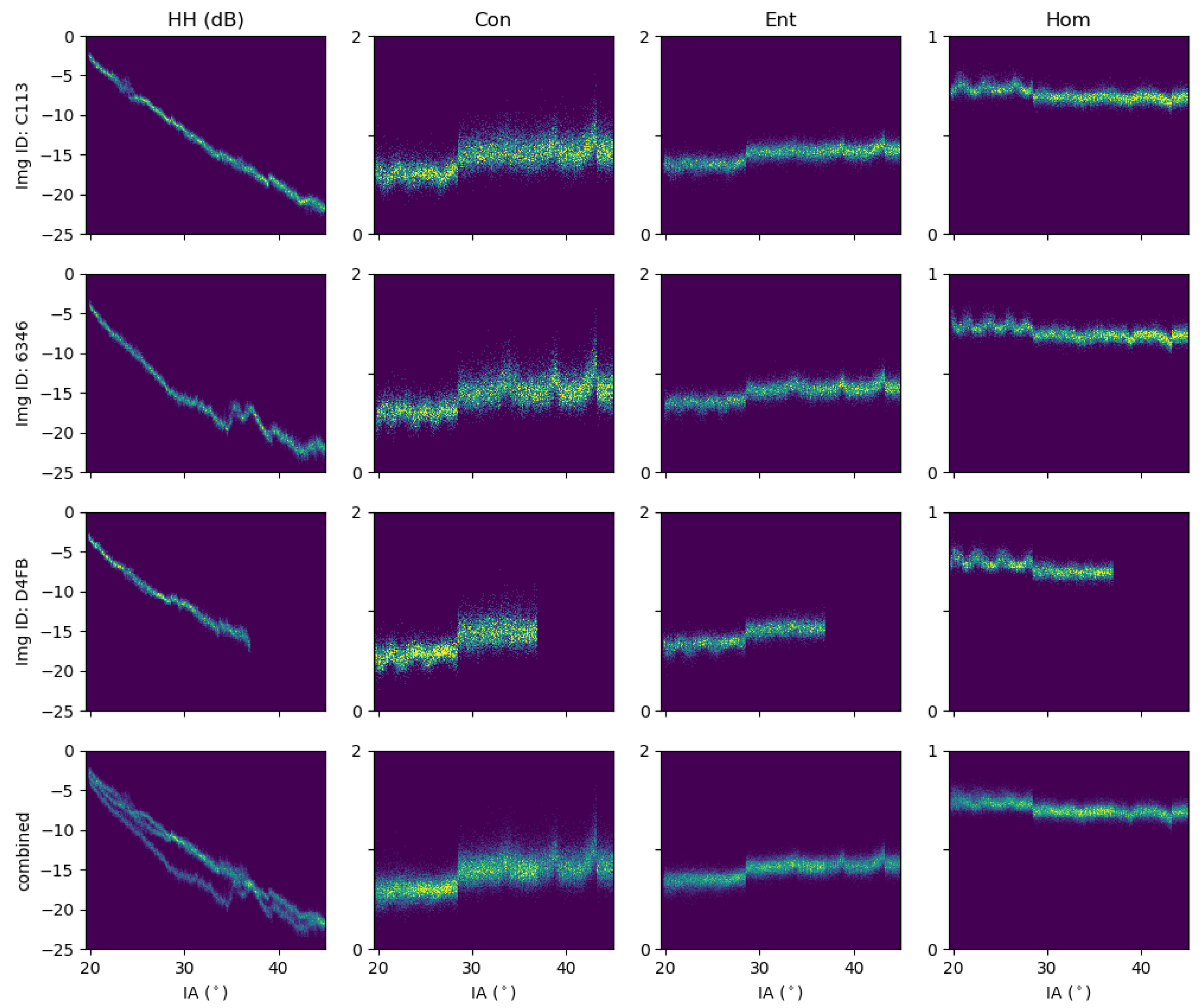
One of the main challenges in sea ice classification is to automatically separate sea ice and OW. As spatial and temporal variations in sea surface state affect the backscatter intensity from OW, a purely intensity-based classifier will often struggle with a generalized separation of sea ice and water, unless additional information is included. We now confirm that texture can help to overcome the issue of different backscatter intensity for varying sea surface states. Figure 6 shows training data of OW areas collected from multiple S1 images. The left column shows the density distributions of HH intensity in dB with IA. Clearly, the intensity levels differed between the images; assuming that the intensity level can be explained by Bragg scattering, its variations can be explained by differences in OW surface roughness. The numerical values of the texture features were consistent over the selected images and wind states (Figure 6, column 2, 3, 4). In agreement with previous results (Figure 4), the numerical texture values and the width of the distributions differed between different GLCM parameter settings (not shown here). Furthermore, the distributions of the texture features remained constant over the IA range, except for the offset between EW1 and EW2.

4.3. Separability of Different Classes

The results presented so far show that the tested GLCM texture features can be directly incorporated into the concept of the GIA classifier, given that the signal is strong enough to avoid noise floor artifacts. The GIA classifier assumes a linear relationship of its features with IA, and an approximately Gaussian feature distribution; thus, the incorporation of GLCM texture features calculated from intensity in dB is straightforward. For the S1 EW GRDM product, the first sub-swath should be ignored or corrected according to the number of looks. However, for the inclusion of the texture features to be useful in terms of improving classification results, we need to investigate the separability of different classes for individual features and varying parameter settings. Note that at this point we are interested in the individual separability of different pairs of classes, as shown on the left side of Table 3. The results of this kind of analysis allow a better understanding of the specific gain achieved by single texture parameters, and they are useful, for example, for designing decision trees such as described in [32].
We performed this analysis by computing the JM distance between the different feature distributions for all settings. Since the HV texture is strongly affected by the noise, we only evaluate texture features extracted from the HH channel at this point. In total, we have analyzed 57 different parameter settings (Table 2) for eight separate features (seven GLCM features (Equations (6)–(12)) and variance). Table 3 presents the JM distance for eight selected parameter settings. Corresponding class distributions for four of these settings are shown in Figure 7.
For the given data set and the parameter settings tested in this study, we found that window size was the parameter with the largest influence on class separability. If a feature offers any separability at all between two tested classes, the separability improves with increasing window size (Table 3 and Figure 7, rows 1, 2, and 5). In agreement with previous studies, we found that many of the tested GLCM features allowed for partial separation of OW from thicker ice types (that is LFYI, DFYI, and MYI). In particular, HH ASM, HH contrast, HH dissimilarity, HH energy, HH entropy, and HH homogeneity all displayed distinct class distributions that revealed at least some separability of LFYI/DFYI/MYI and OW, with JM distance values close to one (for w = 21) and significantly above one (for w = 51).
Figure 8 presents more histogram examples of HH dissimilarity and HH energy for the classes OW and MYI. Again, significant improvement in separability with increasing window size was clearly visible. Separation between the aforementioned thicker ice types (LFYI, DFYI, MYI) is not possible based on the investigated texture features only. This can be seen by the overlapping histograms for LFYI and MYI in Figure 7 (row 4) and was confirmed by the low JM distances between the distributions for all parameter settings and features (Table 3). Partial separation of LFYI and MYI may be possible using the GLCM correlation from the HV channel (Figure 9, right-hand side); however, the HV signal is often close to the nominal noise floor and the channel must be treated cautiously.
None of the tested features separated well between YI and OW. The distributions of these two classes overlapped significantly for all features and all parameter settings (Figure 7, row 3), resulting in low JM distances. However, HH texture showed the potential to improve the classification of MYI against YI in refrozen leads. For several features, JM distances between these two classes were close to and exceeded one at large window sizes (w = 21, 51). Histogram examples of HH dissimilarity and HH energy for YI and MYI are shown on the left-hand side of Figure 9.

4.4. Classification Result Examples

Finally, we demonstrate the potential of including useful texture features in the GIA classifier to improve classification results. On the basis of class separability indicated by the JM distances, we chose different feature combinations and trained the GIA algorithm to classify various test images. Three examples are shown in Figure 10 and Figure 11. The features used for the classification of the presented images were HH intensity, HV intensity, HH contrast, HH dissimilarity, and HH energy. Because of the offset in numerical texture values between sub-swaths EW1 and EW2, we masked out the results for the first sub-swath.
Figure 10 shows all used features (a, b, c, and d) together with the classification result (e) and a map of sea ice concentration (SIC) (f), which can be directly obtained from the classification result. OW and sea ice were well separated in the image, and the ice edge can be successfully detected in both the ice type map as well as the SIC. Some areas within the pack ice were classified as OW; without complementary information, it is difficult to assess whether these areas are in fact OW or YI. Classification of an image containing large OW areas (such as the example in Figure 10) is challenging based on intensity only, as one would need to know the sea surface state to select the correct intensity level and training data for the OW class. Without that additional information, it is only the inclusion of textural information that makes the classification of the image with a generalized classifier feasible. We therefore do not present a result based on intensity only for this case.
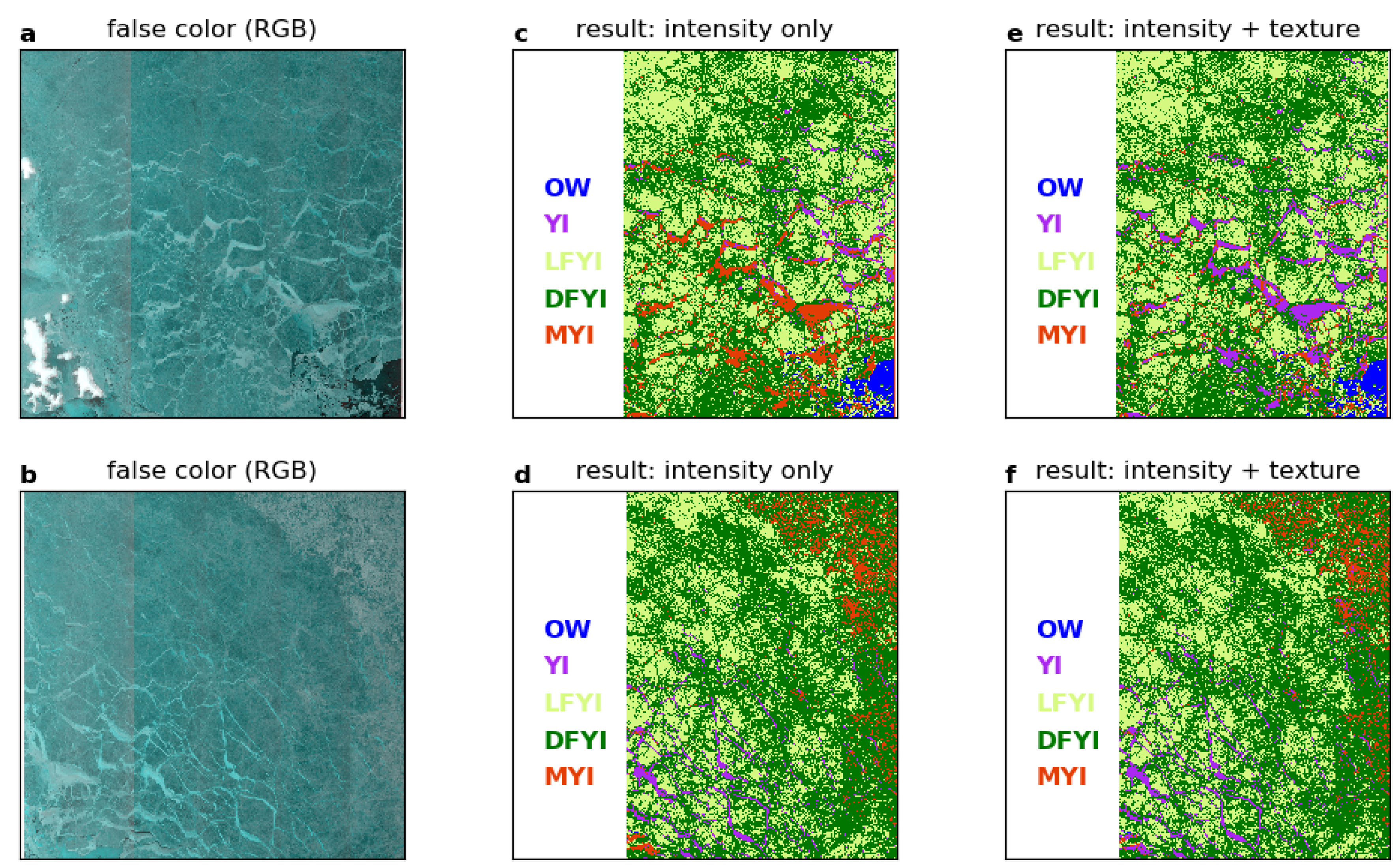
Figure 11 shows false-color images (a and b) and classification results (c, d, e, and f) for two different images that were almost entirely covered by sea ice. The classification results in the middle column (Figure 11c,d) were obtained with a GIA classifier based on intensities only. The same generalized classifier was used for both images. While the classifier captured the YI areas in the lower image correctly (ID B7A9), there was significant mis-classification of YI areas as MYI in the upper image (ID 89A6). This mis-classification occurred despite the fact the YI areas appeared visually similar in both images. A minor change in the properties of the YI areas and thus in the backscatter intensity from the surface can result in the confusion of YI and MYI. The texture signatures of the two classes can help to solve this problem. When the classification was performed including the textural information (Figure 11e,f), the YI areas were classified correctly in both images. The examples demonstrate the superior capability of the GIA classifier using both intensity and texture to separate YI and MYI in situations where the purely intensity-based classifier fails.

5. Discussion

We have investigated the class-dependent variation of different texture features with IA, in order to include them into the GIA classifier. The GIA classifier accounts for per-class variation of its features with IA, and it requires approximately linear relationships and Gaussian distributions. Our results show that it is possible to directly incorporate GLCM texture into the GIA classifier. When computed from intensity in the logarithmic domain (that is in dB), the tested GLCM features do not depend on IA or reveal only a weak, approximately linear dependency. When computed from intensity in the linear domain, the tested GLCM features show considerable variation with IA. For some features the variation is approximately linear over part of the IA range, while for other features it is more complicated. Generally, we therefore recommend to compute texture from the logarithmic intensity; the slope of texture with IA is then constant (approximately zero), and the features can be used in the GIA classifier that assumes a linear relationship. Furthermore, for any other application in a different classification algorithm, as long as texture features are computed from logarithmic intensity, no global correction of the IA effect during pre-processing is needed. We have tested a variety of different GLCM parameter settings and find that the results regarding the IA dependence of the features are independent of the parameter choice. They hold for all tested window sizes, grey levels, and distances. For classes with a weak intensity signal, the S1 noise profile is clearly visible in the distribution of texture features as a function of IA. While this noise pattern will cause problems for any classification algorithm, it is particularly challenging for the GIA classifier, as the basic assumptions of linear IA dependence and Gaussian distributions are violated. The HV channel is more problematic than the HH channel in this regard because the signal at HV polarization is often weak and close to the nominal noise floor. HV texture should thus be used carefully, and it will benefit from an improved thermal noise correction of the S1 data.
Furthermore, we find that there is a distinct offset in all texture features at the sub-swath boundary between EW1 and EW2 of the S1 EW GRDM product. This offset is caused by the different number of looks applied to the individual sub-swaths; the GRDM product is delivered with 18 looks in EW1 and 12 looks in EW2 to EW5. We demonstrate how to correct this offset for the example of GLCM contrast, by multiplying with the square root of the ratio of number of looks in the different EW GRDM sub-swaths. Corrections can also be applied for other GLCM features, but it will depend on the formula for the texture computation. The exact correction factors for all individual features require further investigation and are not part of this study. However, the offset must be considered whenever using texture features extracted from S1 wide-swath products in GRDM format across the full range of the image. Generally, it must be kept in mind that texture is dependent on the speckle contribution in the intensity, and thus on the number of looks in the data.
When integrated into the GIA classifier, GLCM texture features help to resolve some of the inherent ambiguities found with intensity-only classifiers. For example, the general separation of OW and thicker sea ice types, such as LFYI, DFYI, and MYI, is significantly improved by the inclusion of texture. While the backscatter intensity from OW is dependent on the sea surface state and may require the training of several OW classes for different sea surface conditions, the texture signature of OW is nearly independent of the sea state. It suffices to train one OW class for a smooth water surface (where the signal will be close to the nominal noise floor), and one OW class for all rough surface conditions (Figure 6). Another challenge of a classifier based on intensity only is the separation of YI and MYI. Especially for YI with frost flowers or a snow crust, which increases the small-scale roughness and causes strong backscatter from the YI surface, mis-classification of YI as MYI can occur [14,33]. We demonstrate in this study that the inclusion of texture features can significantly improve the separation of YI and MYI.
While some ambiguities of the sea ice type classification can be improved or solved by adding texture features, other classes are not separable in the texture feature space alone. Their per-class texture distributions overlap significantly for all tested features and parameter settings. Hence, backscatter intensity remains an important feature for the classification of these ice types. In particular, this is true for the separation between the thicker ice types (LFYI, DFYI, and MYI), and for the separation of YI and OW. FYI and MYI can be distinguished quite well based on their intensity, as the less saline MYI will cause more volume scattering [34], which results in a stronger signal at both HH and HV polarization. We therefore recommend to always include intensity as a feature in ice type classification. YI and OW, on the other hand, can be more challenging. When the sea surface state, and thus the intensity level of OW, is known, backscatter intensity can be used to overcome this ambiguity. However, since the sea surface conditions are not usually known a priori, the separation of YI and OW remains difficult at this point. We will explore possible solutions such as the inclusion of SIC from passive microwave observations [35] or the results of SAR wind retrieval algorithms [36] in our future work.
The evaluation of features and parameter settings in this study is based on JM distances between different class distributions. Generally, we find that larger window sizes improve the separability between the classes in the used data set. It must be kept in mind, however, that large texture windows result in smoothing and thus in a coarser effective resolution of the results. Hence, there is a trade-off between spatial resolution of the results and separability of sea ice and OW, as well as YI and MYI.
The main focus of our analysis has been on the use of GLCM texture features, as the GLCM method has been widely used for sea ice image analysis [18,20,21,22,23,24,25,26,27]. However, the calculation of the GLCM requires substantial computational resources and is time consuming. For operational ice charting, where timeliness of the results is a main requirement, this can be problematic. We have therefore also tested variance as an example of a more simply calculated texture feature. We find that variance from intensity in dB is roughly independent of IA and can potentially be used as a faster and alternative to GLCM texture. Further investigation of other computationally cheap texture features, such as for example the coefficient of variation or wavelets, is needed in future work and may help to speed up the process of automated sea ice classification, making application of the algorithms feasible in operational ice charting.

6. Conclusions

In this study, we have investigated the IA dependence of seven commonly used GLCM texture features extracted from the S1 EW GRDM product, and we assessed their potential to be included in IA-sensitive sea ice classification (the GIA classifier). When calculated from intensity in dB, the GLCM features are found to be almost independent of IA and can thus be directly included in the GIA classifier, with the estimated slope being approximately zero. Particular attention must be paid to classes with a weak signal, which will lead to noise artifacts in the texture parameters, and to the first sub-swath of the EW GRDM product, as the different number of looks in the sub-swaths results in an offset of texture at the sub-swath boundary. We have shown how this offset can be corrected for the example of GLCM contrast.
We have tested a large number of GLCM parameters and evaluated the resulting features in terms of class separability. Using per-class histograms of feature distributions in combination with the JM distance, we have selected meaningful combinations of texture features and backscatter intensities to train a classifier and demonstrate the improvement in ice-water classification as well as the separation of YI and MYI on various examples compared to classification based on intensity only. Our analysis shows that larger texture windows (up to 51 × 51 pixels) generally result in better class separability, albeit at the cost of reduced spatial resolution of the image.

Author Contributions

Conceptualization, J.L. and A.P.D.; Data curation, J.L. and W.D.; Formal analysis, J.L.; Investigation, J.L., A.P.D. and W.D.; Methodology, J.L. and A.P.D.; Supervision, A.P.D. and W.D.; Validation, J.L., A.P.D. and W.D.; Visualization, J.L.; Writing—original draft, J.L., A.P.D. and W.D.; Writing—review & editing, J.L., A.P.D. and W.D. All authors have read and agreed to the published version of the manuscript.

Funding

This research was funded by CIRFA partners and the Research Council of Norway (grant number 237906). The APC was funded by a grant from the publication fund of UiT The Arctic University of Norway.

Data Availability Statement

Enquiries regarding python code and training data should be made by contacting the first author.

Acknowledgments

The presented work contains primary and altered Sentinel data products (@Copernicus data). We would like to thank the anonymous reviewers for their constructive comments and feedback.

Conflicts of Interest

The authors declare no conflict of interest.

Abbreviations

The following abbreviations are used in this manuscript:
CAclassification accuracy
dBdecibel
DFYIdeformed first-year ice
ESAEuropean Space Agency
EWextra wide
GIAGaussian incident angle classifier
GLCMgrey level co-occurrence Matrix
GRDMground range detected medium
IAincident angle
JMJeffries–Matusita
LFYIlevel first-year ice
MYImulti-year ice
NFInewly formed ice
OWopen water
PDFprobability density function
ROIregion of interest
S1Sentinel-1
SARsynthetic aperture radar
SICsea ice concentration
SNAPSentinel Application Platform
YIyoung ice

References

  1. Ramsay, B.; Manore, M.; Weir, L.; Wilson, K.; Bradley, D. Use of RADARSAT data in the Canadian Ice Service. Can. J. Remote Sens. 1998, 24, 36–42. [Google Scholar] [CrossRef]
  2. Dierking, W. Mapping of Different Sea Ice Regimes Using Images from Sentinel-1 and ALOS Synthetic Aperture Radar. IEEE Trans. Geosci. Remote Sens. 2010, 48, 1045–1058. [Google Scholar] [CrossRef]
  3. Zakhvatkina, N.; Smirnov, V.; Bychkova, I. Satellite SAR Data-based Sea Ice Classification: An Overview. Geosciences 2019, 9, 152. [Google Scholar] [CrossRef] [Green Version]
  4. Dierking, W. Sea Ice Monitoring by Synthetic Aperture Radar. Oceanography 2013, 26, 100–111. [Google Scholar] [CrossRef]
  5. Moen, M.A.N.; Doulgeris, A.P.; Anfinsen, S.N.; Renner, A.H.H.; Hughes, N.; Gerland, S.; Eltoft, T. Comparison of feature based segmentation of full polarimetric SAR satellite sea ice images with manually drawn ice charts. Cryosphere 2013, 7, 1693–1705. [Google Scholar] [CrossRef] [Green Version]
  6. Cheng, A.; Casati, B.; Tivy, A.; Zagon, T.; Lemieux, J.F.; Tremblay, L.B. Accuracy and inter-analyst agreement of visually estimated sea ice concentrations in Canadian Ice Service ice charts using single-polarization RADARSAT-2. Cryosphere 2020, 14, 1289–1310. [Google Scholar] [CrossRef] [Green Version]
  7. Dierking, W. Sea Ice and Icebergs. In Maritime Surveillance with Synthetic Aperture Radar; Institution of Engineering and Technology: London, UK, 2020. [Google Scholar]
  8. Ulaby, F.T.; Moore, R.K.; Fung, A.K. Microwave Remote Sensing: Active and Passive. Volume 1-Microwave Remote Sensing Fundamentals and Radiometry; Addison-Wesley: Boston, MA, USA, 1981. [Google Scholar]
  9. Onstott, R.G.; Carsey, F.D. SAR and scatterometer signatures of sea ice. Microw. Remote Sens. Sea Ice 1992, 68, 73–104. [Google Scholar]
  10. Mäkynen, M.P.; Manninen, A.T.; Similä, M.H.; Karvonen, J.A.; Hallikainen, M.T. Incidence angle dependence of the statistical properties of C-band HH-polarization backscattering signatures of the Baltic Sea ice. IEEE Trans. Geosci. Remote Sens. 2002, 40, 2593–2605. [Google Scholar] [CrossRef]
  11. Gill, J.P.S.; Yackel, J.; Geldsetzer, T.; Fuller, M.C. Sensitivity of C-band synthetic aperture radar polarimetric parameters to snow thickness over landfast smooth first-year sea ice. Remote Sens. Environ. 2015, 166, 34–49. [Google Scholar] [CrossRef]
  12. Mäkynen, M.; Karvonen, J. Incidence Angle Dependence of First-Year Sea Ice Backscattering Coefficient in Sentinel-1 SAR Imagery Over the Kara Sea. IEEE Trans. Geosci. Remote Sens. 2017, 55, 6170–6181. [Google Scholar] [CrossRef]
  13. Mahmud, M.S.; Geldsetzer, T.; Howell, S.E.L.; Yackel, J.J.; Nandan, V.; Scharien, R.K. Incidence Angle Dependence of HH-Polarized C- and L-Band Wintertime Backscatter Over Arctic Sea Ice. IEEE Trans. Geosci. Remote. Sens. 2018, 56, 6686–6698. [Google Scholar] [CrossRef]
  14. Zakhvatkina, N.; Alexandrov, V.Y.; Johannessen, O.M.; Sandven, S.; Frolov, I.Y. Classification of Sea Ice Types in ENVISAT Synthetic Aperture Radar Images. IEEE Trans. Geosci. Remote Sens. 2013, 51, 2587–2600. [Google Scholar] [CrossRef]
  15. Karvonen, J. A sea ice concentration estimation algorithm utilizing radiometer and SAR data. Cryosphere 2014, 8, 1639–1650. [Google Scholar] [CrossRef] [Green Version]
  16. Liu, H.; Guo, H.; Zhang, L. SVM-Based Sea Ice Classification Using Textural Features and Concentration From RADARSAT-2 Dual-Pol ScanSAR Data. IEEE J. Sel. Top. Appl. Earth Obs. Remote Sens. 2015, 8, 1601–1613. [Google Scholar] [CrossRef]
  17. Karvonen, J. Baltic Sea Ice Concentration Estimation Using SENTINEL-1 SAR and AMSR2 Microwave Radiometer Data. IEEE Trans. Geosci. Remote Sens. 2017, 55, 2871–2883. [Google Scholar] [CrossRef]
  18. Zakhvatkina, N.; Korosov, A.; Muckenhuber, S.; Sandven, S.; Babiker, M. Operational algorithm for ice–water classification on dual-polarized RADARSAT-2 images. Cryosphere 2017, 11, 33–46. [Google Scholar] [CrossRef] [Green Version]
  19. Lohse, J.; Doulgeris, A.P.; Dierking, W. Mapping Sea Ice Types from Sentinel-1 Considering the Surface-Type Dependent Effect of Incidence Angle. Ann. Glaciol. 2020, 61, 1–14. [Google Scholar] [CrossRef]
  20. Holmes, Q.A.; Nuesch, D.R.; Shuchman, R.A. Textural Analysis And Real-Time Classification of Sea-Ice Types Using Digital SAR Data. IEEE Trans. Geosci. Remote. Sens. 1984, GE-22, 113–120. [Google Scholar] [CrossRef]
  21. Barber, D.G.; LeDrew, E. SAR Sea Ice Discrimination Using Texture Statistics: A Multivariate Approach. Photogramm. Eng. Remote Sens. 1991, 57, 385–395. [Google Scholar]
  22. Shokr, M.E. Evaluation of second-order texture parameters for sea ice classification from radar images. J. Geophys. Res. Ocean. 1991, 96, 10625–10640. Available online: http://xxx.lanl.gov/abs/https://agupubs.onlinelibrary.wiley.com/doi/pdf/10.1029/91JC00693 (accessed on 1 November 2019). [CrossRef]
  23. Soh, L.K.; Tsatsoulis, C. Texture Analysis of SAR Sea Ice Imagery Using Gray Level Co-Occurance Matrices. IEEE Trans. Geosci. Remote Sens. 1999, 37, 780–795. [Google Scholar] [CrossRef] [Green Version]
  24. Clausi, D.A. Comparison and fusion of co-occurrence, Gabor and MRF texture features for classification of SAR sea-ice imagery. Atmosphere-Ocean 2001, 39, 183–194. [Google Scholar] [CrossRef]
  25. Clausi, D.A. An analysis of co-occurrence texture statistics as a function of grey level quantization. Can. J. Remote Sens. 2002, 28, 45–62. [Google Scholar] [CrossRef]
  26. Deng, H.; Clausi, D.A. Unsupervised segmentation of synthetic aperture Radar sea ice imagery using a novel Markov random field model. IEEE Trans. Geosci. Remote Sens. 2005, 43, 528–538. [Google Scholar] [CrossRef]
  27. Ressel, R.; Frost, A.; Lehner, S. A Neural Network-Based Classification for Sea Ice Types on X-Band SAR Images. IEEE J. Sel. Top. Appl. Earth Obs. Remote Sens. 2015, 8, 3672–3680. [Google Scholar] [CrossRef] [Green Version]
  28. Haralick, R.M.; Shanmugan, K.; Dinstein, I. Textural features for image classification. IEEE Trans. Syst. Man Cybern. 1973, SMC-3, 610–621. [Google Scholar] [CrossRef] [Green Version]
  29. Clausi, D.A.; Deng, H. Operational segmentation and classification of SAR sea ice imagery. In Proceedings of the IEEE Workshop on Advances in Techniques for Analysis of Remotely Sensed Data, 2003, Greenbelt, MD, USA, 27–28 October 2003; pp. 268–275. [Google Scholar] [CrossRef]
  30. Aulard-Macler, M. Sentinel-1 Product Definition S1-RS-MDA-52-7440; Technical Report; MacDonald, Dettwiler and Associates Ltd.: Westminster, CO, USA, 2011. [Google Scholar]
  31. Sen, R.; Goswami, S.; Chakraborty, B. Jeffries-Matusita distance as a tool for feature selection. In Proceedings of the 2019 International Conference on Data Science and Engineering (ICDSE), Patna, India, 26–28 September 2019; IEEE: Piscataway, NJ, USA, 2019; pp. 15–20. [Google Scholar]
  32. Lohse, J.; Doulgeris, A.P.; Dierking, W. An Optimal Decision-Tree Design Strategy and Its Application to Sea Ice Classification from SAR Imagery. Remote Sens. 2019, 11, 1574. [Google Scholar] [CrossRef] [Green Version]
  33. Isleifson, D.; Hwang, B.; Barber, D.; Scharien, R.; Shafai, L. C-band polarimetric backscattering signatures of newly formed sea ice during fall freeze-up. IEEE Trans. Geosci. Remote Sens. 2010, 48, 3256–3267. [Google Scholar] [CrossRef]
  34. Komarov, A.; Buehner, M. Detection of first-year and multi-year sea ice from dual-polarization SAR images under cold conditions. IEEE Trans. Geosci. Remote Sens. 2019, 57, 9109–9123. [Google Scholar] [CrossRef]
  35. Ivanova, N.; Johannessen, O.; Pedersen, L.; Tonboe, R. Retrieval of Arctic sea ice parameters by satellite passive microwave sensors: A comparison of eleven sea ice concentration algorithms. IEEE Trans. Geosci. Remote Sens. 2014, 52, 7233–7246. [Google Scholar] [CrossRef]
  36. Komarov, A.; Zabeline, V.; Barber, D. Ocean surface wind speed retrieval from C-band SAR images without wind direction input. IEEE Trans. Geosci. Remote Sens. 2013, 52, 980–990. [Google Scholar] [CrossRef]
Figure 1. Distribution of HH intensity with IA for OW training data selected over the first two sub-swaths of a single image (Image ID: F2FE). Intensity is shown in the logarithmic domain (in dB) on the left side, and in the linear domain on the right side. The dashed red line indicates the linear fit to approximate the decrease in logarithmic intensity with IA.
Remotesensing 13 00552 g001
Figure 2. Density distribution of HH intensity and three selected GLCM texture features with IA for OW training data selected over the full range of a single S1 image (Image ID: 77 BA). The upper panel shows HH intensity in the logarithmic domain (in dB) and the GLCM features extracted from it; the lower panel shows intensity in the linear domain with its respective GLCM features. Note that the OW class displays some internal class variation in intensity due to varying sea surface state across the image. GLCM parameter settings: w = 11, d = 4, k = 16.
Remotesensing 13 00552 g002
Figure 3. Density distribution of GLCM contrast (computed from HH intensity in dB) with IA for OW training data selected over the full range of a single S1 image (Image ID: F2FE). The left side shows contrast computed directly from the GRDM product; the right side shows contrast manually corrected by multiplying with the square root of the ratio of number of looks in the sub-swaths. The sub-swath boundaries (indicated with red arrows) are clearly visible in the texture profile. In particular the boundary between EW1 and EW2 is characterized by a distinct offset that requires a correction. GLCM parameter settings: w = 21, d = 4, k = 16.
Remotesensing 13 00552 g003
Figure 4. Density distribution of two selected GLCM texture features with IA for MYI training data selected from multiple S1 images. The texture features are computed from HH intensity in dB for different GLCM parameter settings. The first sub-swath EW1 is excluded because of the different number of looks in the GRDM product.
Remotesensing 13 00552 g004
Figure 5. Density distribution of intensity and three selected GLCM texture features with IA for LFYI training data collected from multiple images. The upper panel shows HH intensity in dB and the corresponding HH texture features, the lower panel shows HV intensity in dB and the corresponding texture features. GLCM parameter settings: w = 11, d = 2, k = 16.
Remotesensing 13 00552 g005
Figure 6. Density distribution of HH intensity in dB and three selected GLCM texture features with IA for OW training data selected from three different images (image IDs: C113, 6346, D4FB). The lowest panel shows the data from all three images combined. The intensity values clearly differ between the images, and the texture values are consistent. The offset in texture between sub-swaths EW1 and EW2 is caused by the different number of looks in the respective sub-swaths. The texture artifacts at the remaining sub-swath boundaries are caused by errors in the calibration and noise correction between the sub-swaths. GLCM parameter settings: w = 21, d = 4, k = 16.
Remotesensing 13 00552 g006
Figure 7. Histograms of HH entropy distribution for four selected GLCM parameter settings (one setting per column). For easier interpretation, each row shows only two classes compared against each other. Increasing window size (from left to right) generally leads to narrower distributions and better class separability.
Remotesensing 13 00552 g007
Figure 8. Histograms of HH dissimilarity and HH energy from two different window sizes (w = 21 and w = 51) for OW and MYI. Both features show improved class separability with larger window size.
Remotesensing 13 00552 g008
Figure 9. Histograms of HH dissimilarity, HH energy, and HV correlation for YI against MYI (left) and LFYI against MYI (right). YI and MYI can be partly separated using HH texture. LFYI and MYI are inseparable in HH texture, but can be partly separated in HV correlation, although significant overlap of the distributions remains.
Remotesensing 13 00552 g009
Figure 10. Input features and classification result for image ID F2FE. The scene covers the area across the marginal ice zone in Fram Strait between Svalbard and Greenland. Features used for classification in this example are HH and HV intensity ((a), false-color intensity image [R:HV, G:HH, B:HH]), HH dissimilarity (b), HH contrast (c), and HH energy (d). Sea ice concentration (f) can be calculated directly from the classification result (e). Because of the offset between sub-swaths EW1 and EW2 in the GLCM features (bd), EW1 is masked out in the classification result. GLCM parameter settings: w = 51, d = 4, k = 32.
Remotesensing 13 00552 g010
Figure 11. False-color intensity images ((a,b), [R:HV, G:HH, B:HH]) and classification results using intensities only (c,d) and using intensities in combination with HH dissimilarity, HH contrast, and HH energy (e,f). The top row (a,c,e) shows image ID 89A6, the bottom row (b,d,f) shows image ID B7A9. Both images were acquired over the Arctic Ocean and cover the area northwest of Franz Josef Land. For image ID 89A6, the purely intensity-based classifier mis-classifies many YI areas as MYI (c). The inclusion of texture improves the classification of YI (e). For image ID B7A9, the purely intensity-based classifier captures most of the YI areas correctly (d). The difference to the classification results based on intensities and texture is negligible. Because of the distinct offset between sub-swaths EW1 and EW2 in the GLCM features, EW1 is masked out in the classification result.
Remotesensing 13 00552 g011
Table 1. Overview of GLCM computation parameters from selected studies that investigate GLCM texture features for sea ice classification. The parameters are window size w, co-occurrence distance d, displacement angle α , and number of grey level quantization intervals k. w and d are given in number of pixels, α is given in degrees. Bold type indicates the preferred choice selected by these studies, where applicable. The dB column indicates whether texture was computed from the linear or from the logarithmic intensity. The question mark indicates that this information is not explicitly given in the study.
AuthorsdBwd α kFeatures
Holmes et al. (1984)?52average8Con, Ent
Barber and LeDrew (1991)?251, 5, 100, 45, 9016Con, Cor, Dis, Ent, Uni
Shokr (1991)?5, 7, 91, 2, 3average16, 32Con, Ent, Idm, Uni, Max
Soh and Tsatsoulis (1999)?641, 2, ..., 32average64Con, Cor, Ent, Idm, Uni, Aut
Leigh et al.(2014)?5, 11, 25, 51, 1011, 5, 10, 20average?ASM, Con, Cor, Dis, Ent, Hom, Inv, Mu, Std
Ressel et al. (2015)no11, 31, 651average16, 32, 64Con, Dis, Ene, Ent, Hom
Karvonen (2017)yes51average256Ent, Aut
Zakhvatkina et al. (2017)yes32, 64, 1284, 8, 16, 32, 64average16, 25, 32Ene, Ine, Clu, Ent, Cor, Hom
Table 2. Summary of GLCM computation parameters tested in this study (w: window size, d: GLCM co-occurrence distance, k: GLCM grey levels). The window is applied on the original 40 × 40 m pixel spacing of the S1 EW GRDM product. Quantization is performed with equally spaced intervals between −35 and +5 dB for HH and −40 and 0 dB for HV, respectively. The GLCM is calculated for four different directions (0 , 45 , 90 , 135 ) and then averaged before feature extraction.
wdk
51/216/32/64
71/2/416/32/64
91/2/4/816/32/64
111/2/4/816/32/64
212/4/816/32/64
512/4/816/32/64
Table 3. Jeffries–Matusita (JM) distance between class distributions for multiple combinations of texture features, two-class cases, and parameter settings. Blue and green colors indicate strong JM values above 0.7 and 1.0, respectively. The parameter settings are as follows: Set 1: w = 07, d = 2, k = 16; Set 2: w = 11, d = 2, k = 16; Set 3: w = 11, d = 4, k = 16; Set 4: w = 11, d = 4, k = 32; Set 5: w = 21, d = 4, k = 16; Set 6: w = 21, d = 4, k = 32; Set 7: w = 51, d = 4, k = 16; Set 8: w = 51, d = 4, k = 32.
HH ASMHH ConHH CorHH DisHH EneHH EntHH HomHH Var
Set 10.080.160.030.100.080.120.090.29
Set 20.200.290.110.220.210.290.190.49
OWSet 30.200.360.010.270.220.300.230.49
vs.Set 40.220.390.010.300.240.300.220.49
LFYISet 50.610.700.160.640.630.750.590.85
Set 60.660.730.140.680.680.770.610.85
Set 71.371.280.451.301.351.401.301.27
Set 81.441.290.421.331.411.431.351.27
Set 10.110.210.090.130.120.180.110.48
Set 20.280.360.260.270.310.410.240.75
OWSet 30.300.580.040.430.330.430.360.75
vs.Set 40.330.610.030.480.360.440.350.75
MYISet 50.790.910.290.840.810.900.811.06
Set 60.860.940.260.890.870.930.841.06
Set 71.461.420.591.491.411.431.531.30
Set 81.561.430.541.511.491.451.591.30
Set 10.000.010.000.010.000.000.000.00
Set 20.010.010.010.010.010.010.010.01
OWSet 30.010.010.000.010.010.010.010.01
vs.Set 40.010.010.000.010.010.010.010.01
YISet 50.030.020.050.020.030.040.020.12
Set 60.030.020.050.020.030.040.020.12
Set 70.160.180.540.110.200.360.080.95
Set 80.180.190.510.120.220.340.070.95
Set 10.000.010.010.000.000.010.000.07
Set 20.010.010.040.010.020.030.010.15
LFYISet 30.010.080.010.050.020.030.030.15
vs.Set 40.910.090.010.050.020.030.030.15
MYISet 50.040.130.040.090.050.080.070.27
Set 60.040.140.040.100.050.080.060.27
Set 70.080.210.120.180.100.160.160.38
Set 80.080.210.100.180.090.150.150.38
Set 10.150.270.080.180.150.220.150.51
Set 20.340.440.200.360.360.450.330.68
MYISet 30.350.580.020.460.370.450.400.68
vs.Set 40.390.610.020.500.400.470.400.68
YISet 50.760.880.120.860.750.800.850.81
Set 60.840.900.090.900.820.840.900.81
Set 70.921.160.031.320.860.781.400.23
Set 81.001.170.031.340.940.831.500.23
Publisher’s Note: MDPI stays neutral with regard to jurisdictional claims in published maps and institutional affiliations.