Article

Spatial Retrievals of Atmospheric Carbon Dioxide from Satellite Observations

1
Jet Propulsion Laboratory, California Institute of Technology, Pasadena, CA 91109, USA
2
Department of Statistics, Texas A&M University, College Station, TX 77843, USA
3
Department of Mathematics, Applied Mathematics, and Statistics, Case Western Reserve University, Cleveland, OH 44106, USA
4
Department of Statistics, University of California, Irvine, CA 92697, USA
*
Author to whom correspondence should be addressed.
Remote Sens. 2021, 13(4), 571; https://doi.org/10.3390/rs13040571
Submission received: 31 December 2020 / Revised: 31 January 2021 / Accepted: 2 February 2021 / Published: 5 February 2021
(This article belongs to the Special Issue Advances of Remote Sensing Inversion)

Abstract

:
Modern remote-sensing retrievals often invoke a Bayesian approach to infer atmospheric properties from observed radiances. In this approach, plausible mean states and variability for the quantities of interest are encoded in a prior distribution. Recent developments have devised prior assumptions for the correlation among atmospheric constituents and across observing locations. This work formulates a spatial statistical framework for simultaneous multi-footprint retrievals of carbon dioxide (CO2) with application to the Orbiting Carbon Observatory-2/3 (OCO-2/3). Formally, the retrieval state vector is extended to include atmospheric and surface conditions at many footprints in a small region, and a prior distribution that assumes spatial correlation across these locations is assumed. This spatial prior allows the length-scale, or range, of spatial correlation to vary between different elements of the state vector. Various single- and multi-footprint retrievals are compared in a simulation study. A spatial prior that also includes relatively large prior variances for CO2 results in posterior inferences that most accurately represent the true state and that reduce the correlation in retrieval error across locations.

1. Introduction

Space-borne estimates of atmospheric composition are providing improved understanding of numerous geophysical processes that are closely connected in the climate system. Satellites such as the Greenhouse Gases Observing Satellite (GOSAT) [1] and the Orbiting Carbon Observatory-2 (OCO-2) [2] have provided a multi-year record of global atmospheric carbon dioxide (CO2) concentration that is improving quantitative inferences for the carbon cycle [3]. The recently launched OCO-3 satellite facilitates small-area investigations over areas such as megacities [4]. These high-resolution satellite products can ultimately be used in flux inversion systems to infer carbon sources and sinks, potentially at regional scales [5,6]. The end-to-end processing pipeline from satellite spectra (Level 1) to inferred carbon fluxes (Level 4) includes multiple stages of inference that require robust uncertainty quantification [7].
An observation made by the OCO-2 instrument at a particular location consists of a spectrum, which is a vector y of calibrated radiances based on photon counts at different wavelengths. From this spectrum, the goal is to infer a state vector x , which includes CO2 concentrations at different altitudes, along with other atmospheric and surface constituents within the instrument field of view, or footprint, which is 1.3 × 2.25 km in nadir mode. The OCO-2 retrieval algorithm infers the state vector from the observed spectrum by solving an inverse problem involving a physical forward model, which relates the state vector to the spectrum. The forward model is combined with a prior assumption on the state in a Bayesian framework known as optimal estimation (OE) in the remote-sensing literature [8]. Operational algorithms for OCO-2/3 perform this retrieval one location (footprint) at a time [9,10]. Since this retrieval approach produces Level 2 data products, we will refer to this operational retrieval as the L2 retrieval.
The unknown state that is inferred in the L2 retrieval includes atmospheric, surface, and instrument characteristics. The atmospheric state is represented by a vertical profile of CO2, along with surface pressure and aerosol profiles. The observed satellite spectra alone do not provide sufficient information to infer the full unknown state, making the retrieval an ill-posed inverse problem. The OE methodology uses prior information to provide regularization. The primary quantity of interest (QOI) is XCO2, the column-averaged dry-air mole fraction of CO2. A ground-based network known as the Total Carbon Column Observing Network (TCCON) [11] provides validation for the OCO-2/3 retrievals. Further, since atmospheric CO2 varies smoothly (horizontally) in space over long ranges in areas with minimal sources/sinks, such as the oceans of the Southern Hemisphere, analysis of retrievals in small spatial areas provides insight into the potential spatial correlation of retrieval errors [12,13,14]. The inherent spatial dependence in the true geophysical process of interest and the presence of spatially correlated retrieval errors motivate interest in a retrieval methodology involving multiple locations simultaneously. Here, we propose the development and testing of a spatial retrieval algorithm that carries out a joint retrieval for all pixels in a given region by exploiting the fact that CO2 values at two neighboring pixels should be very similar to each other; that is, the CO2 field exhibits strong spatial dependence, particularly in the absence of strong sources and sinks.
We expect our spatial retrieval approach to deliver several advantages relative to the current retrieval algorithm: (1) The retrieved CO2 values at each pixel should be closer to the truth. (2) We expect the derived uncertainties to be more reflective of the actual discrepancies between the retrieved and true values. (3) Spatial retrievals allow a characterization of the spatial dependence in the retrieval errors. (4) We expect that this spatial dependence in the errors is reduced, which is very important for follow-up analyses, such as flux inversion. (5) As spatial retrievals allow regularization of the retrieval problem in the “horizontal” direction, they might allow a relaxation of the regularization along the dimension of the state vector, hence making the retrieval less dependent on a priori assumptions related to the state.
The methodology for multi-footprint retrievals has been employed for data from multi-angle polarimetric instruments focused on estimating atmospheric aerosol information, including for joint retrieval of aerosol and surface parameters from POLDER/PARASOL [15] and for retrievals from airborne campaigns with the Airborne Multiangle SpectroPolarimetric Imager (AirMSPI) [16]. A multi-footprint retrieval approach is planned for the retrieval of aerosol parameters for the Multi-Angle Imager for Aerosols (MAIA) mission [17]. The general idea of a multi-footprint retrieval was also recently suggested in [7].
The multi-footprint aerosol retrieval efforts [15,16] combine information across multiple footprints, viewing angles, and polarizations to infer multiple aerosol properties. Even with this rich spectral information, the retrieval inverse problem remains ill-posed, and the authors invoke a collection of spectral and spatial smoothness constraints in addition to within-footprint state variable constraints in the spirit of OE [8]. In particular, Ref. [15] imposes smoothness constraints on aerosol parameters enforced by finite differences of neighboring footprints. An extension developed in [16] provides additional focus on the within-footprint correlation structure of aerosol parameters, which are captured via constraints on principal components (PCs) of the aerosol states. The multi-footprint joint aerosol and surface retrieval has also been implemented for observations from GOSAT over urban areas [18]. Other OE retrievals that combine multiple observations across space have been developed for limb sounders [19], which have a particular focus on trace gas retrievals in the upper atmosphere.
In this work, we motivate the multi-footprint retrieval with a focus on a hierarchical statistical model for a remote-sensing observing system [7,20]. In this context, a multivariate spatial model for the joint distribution of the state is formulated. Recent research in multivariate spatial statistical modeling has provided flexible models that would have utility in inverse remote-sensing problems. Importantly, these multivariate spatial models allow the smoothness and correlation range of the spatial process to vary across variables of the state while maintaining a valid joint probability distribution [21]. This property is particularly applicable to the heterogeneous state vector considered in a remote-sensing retrieval. For example, CO2 concentration near the surface in the presence of sources and sinks may have a different correlation range than concentration higher in the atmosphere where it is well mixed. Further, other state vector components, such as surface albedo, are likely to vary on spatial scales different from those of atmospheric constituents.
We invoke a Gaussian-process-based regularization with the Matérn covariance structure to incorporate the spatial dependency in the model. The Matérn covariance model has been widely used in spatial statistics. For a univariate spatial process, the model is parameterized by a range parameter λ that dictates the rate of decay of spatial correlation with distance and a smoothness parameter ν that characterizes the differentiability of the process. The exponential covariance function is a special case with ν = 0.5 [22]. This type of covariance structure has no boundary effects, and thus allows us to straightforwardly specify a joint spatial model that can incorporate different degrees of smoothness for the CO2 concentrations at different pressure levels. Modeling the cross-covariance in the spatial structure is a major contribution of our article in this regard. In statistical terms, the constraint-based spatial retrieval formulation [15] corresponds to a Gaussian Markov random field (GMRF), specifically the conditional autoregressive (CAR) model [23]. A GMRF prior is also considered in hierarchical Bayesian retrievals of aerosol optical depth (AOD) from spectra observed by the Multi-angle Imaging Spectro Radiometer (MISR) [24,25]. The intrinsic GMRF implied through these spatial priors produces a somewhat inflexible spatial correlation structure, and the models we investigate offer additional flexibility.
The remainder of this paper is organized as follows. In Section 2, we introduce the multi-footprint retrieval methodology and mathematical notation in the context of OCO-2. Section 3 describes a collection of simulation experiments that investigate the spatial retrieval for CO2 using a reduced-order linear model. Section 4 provides concluding remarks and prospects for future work.

2. Spatial Retrieval Methodology

We consider spatial retrievals for a set, S = { s 1 , , s n } , of n footprints along a short span of a single OCO-2 polar orbit. Each footprint is indexed by geolocation information (longitude, latitude) s i . Figure 1 shows an example of a small area for an OCO-2 orbit that passed near the Lamont, OK TCCON site in October 2015. This density of observations within a small spatial domain in OCO-2’s standard observing mode, as well as observations made in its target mode, are valuable for validation as well as for regional carbon cycle studies [26,27]. In this section, we outline the mathematical framework for estimating CO2 concentration from the satellite spectra in the operational retrieval configuration and provide an extension to a multi-footprint spatial retrieval.

2.1. Model and Notation

At a single footprint s i , the state of the atmosphere and surface is represented as a p-dimensional vector x ( s i ) = x 1 ( s i ) , , x p ( s i ) . In addition to CO2 concentration, other variable and unknown atmospheric constituents are included in the state vector for OCO-2. The additional elements include atmospheric aerosols, surface albedo, and surface air pressure. The numerical investigation in Section 3 examines an implementation with p = 39 [20]. The collection of state vectors in the small area is assembled into an n p -dimensional vector,
x ( S ) = x ( s 1 ) , , x ( s n ) .
The spectrum observed by the satellite is an m-dimensional vector y ( s i ) . For a single footprint, OCO-2 observes radiances of up to m = 3048 spectral channels. The spectra are observed in three narrow infrared bands: the O2 A-band at 0.76 μm, the weak CO2 band at 1.61 μm, and the strong CO2 band at 2.06 μm. Each band corresponds to a different spectrometer on OCO-2 and has up to 1016 channels. The vector y ( S ) represents the set of all spectra at locations in S . The physical relationships between the state and the spectra are contained in a forward model F ( · ) . In general, the forward model is nonlinear.

2.2. The Spatial Objective Function

Many modern retrievals implement a Bayesian framework to infer the atmospheric state from the observed satellite spectra. The L2 retrieval implements an OE methodology for a single footprint at a time. Extending this assumption of independence across footprints, the L2 retrieval algorithm for a collection of footprints maximizes the objective function
g x ( S ) = i = 1 n N x ( s i ) | μ i , Σ i N y ( s i ) | F ( x ( s i ) ) , V i
with respect to x ( S ) , where N · | μ , Σ denotes a multivariate normal (Gaussian) density with mean μ and covariance matrix Σ . The statistical assumptions of a normal prior on the state and a normal data model for the spectra given the state are typical for OE retrievals [10]. Here, V i is a diagonal matrix containing the measurement-error variances, and μ i and Σ i are the prior mean vector and covariance matrix of x ( s i ) , respectively. The off-diagonal elements of the p × p matrix Σ i characterize the dependence between different elements of the state vector (i.e., between CO2 at different pressure levels and the other state variables). This prior covariance matrix controls the regularization along the dimension of the state vector, and can be viewed as a “vertical” regularization for the CO2 profile. Since the forward model is nonlinear, the objective function is optimized numerically and separately for each i using an algorithm, such as gradient descent, Gauss–Newton, or Levenberg–Marquardt [8].
The spatial retrieval instead maximizes the spatial objective function
g S x ( S ) = N x ( S ) | μ , Σ i = 1 n N y ( s i ) | F ( x ( s i ) ) , V i
with respect to x ( S ) , where μ ( μ 1 , , μ n ) , and Σ is a joint n p × n p covariance matrix with diagonal blocks Σ i (as above) and ( i , j ) th off-diagonal block c o v ( x ( s i ) , x ( s j ) ) . These off-diagonal blocks characterize the spatial dependence of CO2 and other variables in the state vector. This allows us to borrow strength over space. These off-diagonal blocks can be viewed as a “horizontal” regularization. This spatial retrieval strategy has been implemented in multi-footprint retrievals for aerosols in particular [15,16]. These approaches have typically achieved this regularization with spatial smoothness constraints rather than with a spatial statistical model. Even so, the spatial smoothness constraints can be viewed as specific structures for the prior covariance matrix Σ . More generally, parameterizing the cross-correlations offers additional flexibility in the retrieval, but can be challenging. A strategy for the OCO-2 small areas is discussed in Appendix A.1.

2.3. State Vector

The radiances observed by OCO-2/3 are sensitive to a number of atmospheric, surface, and instrument properties that are unknown and that vary spatially. These properties are represented in the state vector x ( s i ) . In the simulation study in Section 3, a state vector of dimension p = 39 following [20] was used. The state vector is composed of four distinct groups of geophysical elements, as outlined in Table 1. The state includes an atmospheric vertical profile of CO2, surface air pressure, atmospheric aerosols of varying types, and wavelength-dependent surface albedo in the three spectral bands. Further details on this configuration can be found in [20]. This slightly simplified state vector omits some elements in the full physics state vector [10].
In extending the retrieval to a multi-footprint framework, it is important to consider the nature of spatial dependence for the various elements of the state vector. The horizontal spatial correlation length scale for CO2 varies vertically. Near the surface, atmospheric CO2 can be highly variable in the presence of surface sources or sinks. At higher altitudes, away from direct sources and sinks, CO2 can have larger correlation length scales [28,29]. Aerosols are similarly sensitive to atmospheric transport, but have generally shorter residence times. Surface pressure and clouds have spatial scales connected to weather systems. Surface albedo over land can have short correlation length due to heterogeneity in surface types. A multi-footprint retrieval methodology should have the capability for spatial dependence that varies with the state vector element.
While the OCO-2/3 retrieval estimates multiple atmosphere and surface constituents, the mission’s primary quantity of interest is known as XCO2, which is the column-averaged dry-air mole fraction of CO2. This quantity is a weighted average of the CO2 vertical profile portion of the state vector,
XCO 2 ( s i ) = h T x ( s i ) .
The distribution of XCO2, given a Gaussian distribution for x ( s i ) , is given by:
XCO 2 ( s i ) N ( h T E x ( s i ) , h T V a r [ x ( s i ) ] h ) = N ( μ XCO 2 , σ XCO 2 2 )
By plugging in the posterior distribution for XCO 2 ( s i ) , this formula can be used to evaluate our proposed procedure as a log score (see Section 3.2).

2.4. A Tractable Linear Model

We consider the special case of a linear forward model that can be described by a matrix, F S . We then have the Bayesian model x ( S ) N ( μ , Σ ) and y S | x ( S ) N ( F S x S , V ) , where V = b l o c k d i a g ( V 1 , , V n ) . That is, the measurement noise for an individual footprint is assumed to be uncorrelated with that for any neighboring footprints. Similarly, we have essentially assumed F S to be block-diagonal as well. This structure is consistent with a 1D (vertical atmospheric path) radiative transfer model. We make this assumption for the land nadir observations considered in the current work.
In this simple linear case, we can write down the posterior of x S in closed form: x S | y S N ( μ x | y , Σ x | y ) , where Σ x | y 1 = Σ 1 + F S V 1 F S and μ x | y = μ + Σ x | y F S V 1 ( y S F S μ ) .
We can now examine the effects of Σ and/or F S being (incorrectly) assumed to be block-diagonal.
  • If F S is block-diagonal, then so is F S V 1 F S .
  • If Σ is block-diagonal, then so is Σ 1 .
  • If both are block-diagonal, then so are Σ x | y 1 and Σ x | y . This would imply that dependence across footprints is being ignored. Further, the posterior covariances for individual footprints will typically be incorrect.
In addition, note that the smaller the noise variance V , the less the prior covariance Σ matters. So, the effect of using a spatial prior will be most pronounced if Σ is “small” relative to V .

2.5. Considerations for Degeneracy

If the prior state components are highly correlated across space, the prior covariance Σ may become nearly singular and require special handling. This is often the case after performing the multivariate spatial estimation procedure outlined in Appendix A.1. This issue can be circumvented with a low-rank model based on principal components, which is an approach used in other multi-footprint retrievals [16]. The covariance matrix is written as a product of diagonal standard deviation matrices S and a correlation matrix C ,
Σ = S C S ,
so that the highly correlated elements are directly accessible.
Performing an eigen-decomposition of C , we take the top e eigenvalues that explain sufficient variation and exclude all remaining terms. The result is written as Σ S P e D e P e S , where P e is the n p × e matrix of the top e eigenvectors of the correlation C , and D e is the diagonal matrix of the e leading eigenvalues.
Propagating this low-rank prior in the original state vector space as if it were the original prior is not feasible because it has a singular covariance, and any step involving the precision matrix would fail. We instead reparameterize the model using x S S P e x ˜ + μ , where x ˜ N ( 0 , D e ) represents the lower rank latent space and cannot be directly interpreted. Using standard techniques, the posterior distribution for x ˜ can be shown to take the form x ˜ | y = N ( μ ˜ x | y , Σ ˜ x | y ) , with
Σ ˜ x | y = [ S P e F V 1 F P e S + D e 1 ] 1
μ ˜ x | y = Σ ˜ [ S P e F V 1 ( y F μ ) ]
Converting back into the original state vector space only requires the reparameterization,
E ( x S | y ) S P e μ ˜ x | y + μ
and a similar formula for the variance: V ( x S | y ) S P e Σ ˜ x | y P e S .

3. Numerical Study

In this section, we present a collection of simulation experiments to assess the performance of the multi-footprint retrieval methodology. The simulations are carried out over spatial domains corresponding to small areas within individual OCO-2 orbits (Figure 1). Multiple retrieval approaches are compared for each of three small area templates.

3.1. Simulation and Retrieval Configuration
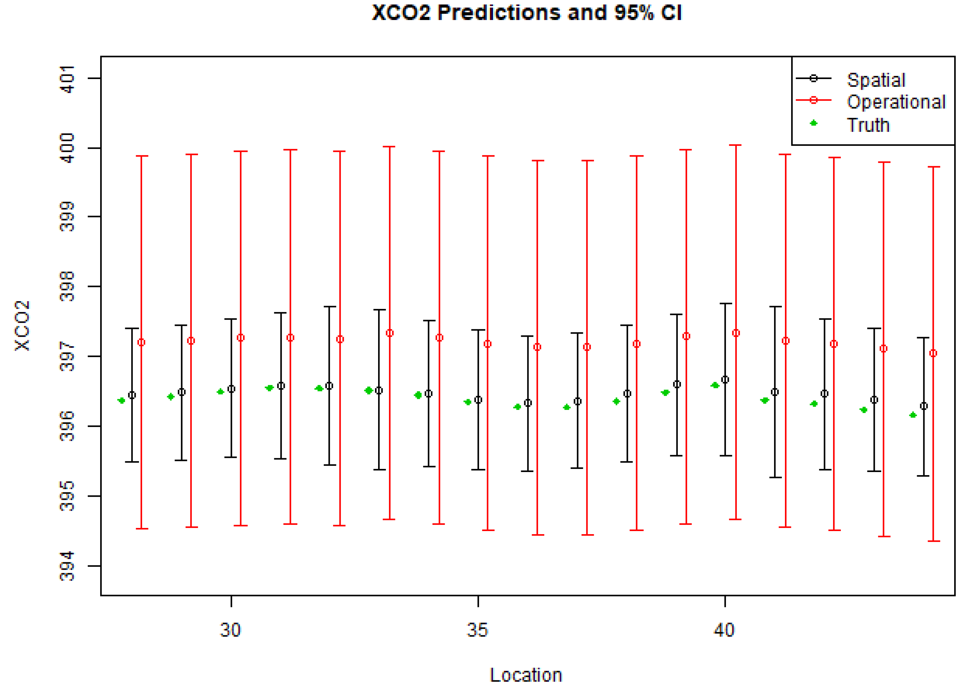
We estimated a realistic covariance structure for the spatial distribution of the state at three space–time locations that coincide with TCCON sites; one in Lamont, OK, USA and two in Wollongong, Australia. The procedure for estimating the spatially informed covariance Σ from available data is rather involved and is described in Appendix A.1. The estimated spatial correlation range parameters for each template and state vector element are shown in Figure 2. The estimated range parameters are generally tens of kilometers for most state vector elements, but differences exist among state elements and across the three geophysical templates. Surface albedo correlation ranges are typically smaller than those for atmospheric constituents, such as CO2 and aerosols.
The procedure also yields an estimate for the mean vector μ . For the purposes of the numerical study, these parameters are denoted μ T and Σ T and serve as the “true” data-generating parameters for the study. The true mean vectors μ T , along with the operational prior means μ a , are summarized for the three templates in Figure 3 and Table 2. The true mean differs from the prior mean in meaningful ways for XCO2, as well as for other key state vector elements, such as surface pressure.
A small OCO-2 area is identified for each of the three TCCON coincidences. The locations form an 8 × 8 grid that resembles the swath over which the satellite would have collected observations. For each case, an ensemble of spatially correlated state vectors is randomly generated as x S N ( μ T , Σ T ) from the reparameterized multivariate Gaussian prior described in Section 2.5, which has mean and variance parameters estimated following the procedure in Appendix A.1. Since each state vector has 39 components, each sample corresponds to 39 × 64 = 2496 values. For each simulated multivariate field, an ensemble of synthetic radiances is generated from a linear forward model based on the surrogate forward model of [20].
Finally, a series of single-footprint and spatially informed retrievals are carried out on the simulated radiances. For each retrieval, the assumed prior mean vector, denoted by μ a , is taken to be the OCO-2 operational prior mean for the appropriate time and location. Importantly, the prior mean is not equal to the true mean, μ a μ T . This is a realistic situation and has potential impacts on the retrieval bias [30]. Three different choices for the prior covariance Σ a are investigated:
  • Operational, Σ a = I 64 Σ a , 0 , where I 64 is an identity matrix with a dimension matching the number of spatial locations. The OCO-2 operational prior covariance for a single footprint, Σ a , 0 , is used at all locations, assuming no spatial correlation. This is essentially a single-footprint retrieval. In this case, the prior standard deviations for the CO2 profile are substantially larger than those in Σ T (see Figure 3 of [30]).
  • Spatial, Σ a = S a C a S a . The within-footprint operational correlation structure is extended between footprints by averaging parameters (see (A1) in Appendix A.1), yielding a multivariate spatial correlation matrix C a . This is combined with the standard deviations used in the operational retrieval, represented in the diagonal matrix S a .
  • True, Σ a = Σ T . The prior covariance is set to the true data-generating spatial covariance.
The true data-generating covariance Σ T and the spatial covariance Σ a both exhibit numerical instability, so low rank approximations are used, as discussed in Section 2.5. Using 200 dimensions for Σ T and 1000 dimensions for Σ a at each site recovered at least 99% of the variability across all scenarios. For additional numerical stability, the estimated range and smoothness parameters for the Matérn covariance function are truncated to numerically stable intervals of [ 0 , 25 ] for the range and [ 0.5 , 1.5 ] for the smoothness.

3.2. Results

Here, we summarize the results of the retrieval simulation experiments for the three TCCON templates. Several properties of the retrievals are relevant in this multivariate spatial setting. First, the retrieval properties for the various state vector elements at a single spatial location are summarized. Figure 4 shows the logarithm of the mean squared error (MSE) by the state vector element for a single pixel in the October 2015 Lamont experiment. The log MSE is shown in part due to the changing magnitudes of variability for the various state vector elements. The spatial prior tended to improve MSE, especially for spatially correlated parameters, such as the atmospheric components. However, using the highly informative true covariance in the prior can be detrimental to retrieval performance, as the prior mean misspecification contributes to bias in this scenario [30].
The different retrieval methods also yield different retrieval behaviors across the entire spatial domain. Two important aspects of the spatial behavior for the retrieval of XCO2 are illustrated in Figure 5 and Figure 6. The spatial retrievals result in smaller retrieval-error standard deviations, which is illustrated through XCO2 credible intervals for a portion of the October 2015 Lamont template in Figure 5. Science investigations that use OCO-2 data involve combining retrievals in various ways [3], and an understanding of the correlation of retrieval errors is often critical. Figure 6 displays a series of correlation matrices of the XCO2 retrieval error for the three choices of prior covariance. The operational single-footprint approach yields errors that are strongly spatially correlated, while the spatial prior reduces spatial correlations in the error for the October 2015 Lamont case. Figure 7 summarizes the mean absolute error (MAE) for XCO2 by location for the Lamont template. While the errors are relatively uniform across the small area, they are smallest in magnitude near the center, where the spatial retrieval provides the most information from surrounding locations.
We aggregate the results for XCO2 across multiple simulations in Table 3 by computing the mean squared error (MSE) and two forms of a mean log score. The log score evaluates the likelihood of the generated truth given the posterior distribution implied by the retrieval (e.g., [31]). These scores are examples of proper scoring rules or metrics that characterize predictive distributions. In practical terms, proper scoring rules are optimized when predictive distributions are as narrow as possible while still capturing the true state for a sufficient percentage of the time. The marginal log score uses the variance of the XCO2 estimate for each location, ignoring the off-diagonal covariance terms relating XCO2 measurements at different locations. For example, with 100 generated samples x S , the joint L and marginal log scores m L are
L ( { XCO 2 ( k ) ( S ) } k = 1 100 ) = k = 1 100 log N ( XCO 2 ( k ) ( S ) | μ XCO 2 | y ( k ) , Σ XCO 2 | y ( k ) ) ,
m L ( { XCO 2 ( k ) ( S ) } k = 1 100 ) = k = 1 100 i = 1 64 log N ( XCO 2 ( k ) ( s i ) | μ XCO 2 | y ( k ) , σ XCO 2 | y ( k ) ) .
Here, σ XCO 2 | y ( k ) corresponds to the ith diagonal component of the k t h simulation realization’s XCO2 posterior covariance Σ XCO 2 | y ( k ) . Since the operational prior assumes independence across footprints, the joint and marginal scores will be the same for this prior choice. For all three templates, the spatial prior yields the most desirable outcomes for both the marginal and joint scores. The scores are consistent with Figure 4, showing that using the true covariance as the prior is far too optimistic due to the prior mean misspecification.
Although it is of secondary interest, we also compute a mean absolute error (MAE) and MSE for the posterior estimate of the full state vector in case one of the components not related to XCO2 is poorly estimated. Performance for the full state is consistent with the XCO2 estimates. The important takeaway from this simulation is that the improvement in posterior accuracy and precision due to a spatial model is closely related to the covariance parameters. As the parameters strengthen cross-correlation, the benefit of a spatial model becomes more obvious.

4. Discussion

We have developed a multi-footprint retrieval approach for estimating atmospheric CO2 from remote-sensing observations over small spatial areas. The statistical properties of the retrieval approach were investigated with simulation experiments with a realistic simplified physical forward model. A prior that combines spatial correlation across footprints with a large prior variance for individual levels of the CO2 vertical profile often provides improved precision over single-footprint retrievals (Figure 5). In addition, the multi-footprint approach can reduce the spatial correlation of retrieval errors, which enhances utility for downstream scientific use of the retrieval results [3].
The multi-footprint retrieval approach has demonstrated utility for other remote-sensing applications [15,16], and the methodology in this work can set the stage for further development of spatial retrievals for CO2 and other trace gases. Our simulations suggest that the actual spatial dependence as well as the assumed spatial dependence in the prior retrieval distribution have an impact on the retrieval precision and magnitude of spatial correlation in retrieval errors. Widespread implementation would need additional investigation of these interactions, as well as of the role of the within-footprint correlation structure. The multi-footprint retrieval may have added value in situations that are challenging for the current single-footprint retrieval, including low signal-to-noise situations, such as dark surfaces and high-latitude observations [32].
Other aspects of the observing modes for OCO-2 and OCO-3, as well as other greenhouse-gas-observing missions, could benefit from the multi-footprint retrieval approach. Both OCO-2 and OCO-3 periodically observe in target mode, where multiple observations at varying geometries are collected over an area near a validation site (e.g., TCCON) in a short time span [33]. Further, OCO-3 uses a pointing mirror assembly (PMA) for observations at varying geometries and has instituted a two-dimensional sweeping mode known as snapshot area mode (SAM). These modes produce observations over small spatial regions and could be combined by invoking prior distributions that account for inherent spatial dependence in the surface and atmospheric states. In addition, the spatial coverage of OCO-2/3 retrievals is incomplete in the presence of clouds. Cloudy footprints are typically screened out before the retrieval is attempted. A multi-footprint approach would still not use cloudy radiances, but could provide a mechanism for inferring conditions given nearby clear scenes.
There are several parameters in F , V i , μ i , and Σ that need to be estimated in order to implement the multi-footprint retrieval methodology. In principle, it would be possible to do this online as part of the multi-footprint retrieval with the aid of a hierarchical statistical model [7]. However, this might be quite computationally challenging, and would likely require joint retrievals for very large spatial fields as well as additional tools for Bayesian inference, such as Markov-chain Monte Carlo methods. Currently, the within-pixel parameters are estimated offline based on different sources of information and expert knowledge (Appendix A.1).
Using OCO-2 Level 2 products for characterizing the multivariate and spatial dependence of the state (i.e., the off-diagonal blocks in Σ ) has inherent advantages and disadvantages. The OCO-2 products have the necessary spatial resolution and span the ranges of the plausible geophysical conditions anticipated. The estimation procedure outlined in Appendix A.1 aims to account for some artifacts introduced by the ill-posed nature of the retrieval, but remaining information on spatial correlation can still be limited, particularly for the retrieved CO2 [14]. The additional parameters necessary for spatial retrievals could be estimated offline using atmospheric transport models [34] if the spatial resolution is suitable.
The current study has demonstrated some statistical properties of the multi-footprint retrieval for a linear forward model. Combined with the assumed Gaussian distributions, this setting provides tractable analytical results. In the operational setting, the forward model is moderately nonlinear, and the retrieval involves iterative numerical optimization. The forward-model evaluation on successive iterations adds noticeably to the computational expense of the retrieval. In a multi-footprint setting, the cost function (2) requires evaluation of the forward model for all footprints. Any computational gains or losses would depend on the overall number of iterations for the spatial retrieval. These and other operational computational challenges warrant further investigation.
If it turns out that more iterations of the nonlinear-least-squares solver are necessary for the same degree of convergence, there are several compromises that could be made to reduce the computational effort. First, we could use a statistical emulator of the forward model to obtain good starting values for the algorithm. Second, it is, of course, always possible to run the optimization for only a fixed number of iterations, at which point the achieved solutions might still be better than the current retrievals at the same computational effort. Finally, we could carry out “sequential retrievals”, meaning single-pixel retrievals conditioned on the previous retrievals, as opposed to the simultaneous multi-pixel retrievals proposed above. More specifically, based on some ordering of the pixels in a small region, a regular retrieval would be carried out for the first pixel. The resulting posterior distribution, together with the assumption of spatial dependence, would then imply a prior distribution for the next pixel, which would be “tighter” (i.e., more peaked and informative) than the original prior, and so forth.
The multi-footprint retrieval provides additional regularization of the joint atmosphere and surface state in the horizontal spatial dimension. This constraint could enable relaxation of the regularization within a single footprint, particularly for the vertical profile of CO2. The use of the larger-variance spatial prior in Section 3.1 provides an initial investigation of this idea, but further adjustments to the within-footprint correlation structure could prove useful. This investigation would be valuable for the CO2 retrieval problem as well as for the retrieval of vertical profiles of other trace gases, such as O3 and CH4.

Author Contributions

J.H.: Project administration, Methodology, Software, Validation, Formal analysis, Data curation, Writing—original draft, Writing—review and editing, Visualization. M.K.: Conceptualization, Methodology, Supervision, Writing—original draft, Writing—review and editing. D.Z.: Methodology, Investigation, Software, Validation, Formal analysis, Data curation, Writing—original draft, Writing—review and editing, Visualization. J.B.: Conceptualization, Methodology, Investigation, Software, Formal analysis, Writing—review and editing. A.M.: Conceptualization, Methodology, Investigation, Formal analysis, Writing—review and editing. V.B.: Conceptualization, Methodology, Investigation, Writing—review and editing. All authors have read and agreed to the published version of the manuscript.

Funding

This work was performed at the Jet Propulsion Laboratory of California Institute of Technology under contract with NASA. Support was provided by the Orbiting Carbon Observatory-2/3 (OCO-2/3) missions.

Data Availability Statement

The data for the simulations presented in this study are available on request from the corresponding author. OCO-2 data products are publicly available available at the NASA Goddard Earth Science Data and Information Services Center (GES DISC) https://disc.gsfc.nasa.gov/datasets?page=1&keywords=OCO-2.

Acknowledgments

This collaboration originated during the Statistical and Applied Mathematical Sciences Institute (SAMSI) program on Climate and the Earth System. The authors appreciate the program leadership provided by Richard Smith, Amy Braverman, and Jessica Matthews. The authors thank Noel Cressie, Annmarie Eldering, Michael Gunson, Susan Kulawik, Mikael Kuusela, James McDuffie, Vijay Natraj, Pratik Patil, and John Worden for valuable suggestions and technical assistance. The comments from the three reviewers improved this paper.

Conflicts of Interest

The authors declare no conflict of interest. The funders had no role in the design of the study; in the collection, analyses, or interpretation of data; in the writing of the manuscript, or in the decision to publish the results.

Abbreviations

The following abbreviations are used in this manuscript:
AirMSPIAirborne Multiangle SpectroPolarimetric Imager
AODAerosol Optical Depth
CARConditional Autoregressive
GMRFGaussian Markov Random Field
GOSATGreenhouse Gas Observing Satellite
GPGaussian Process
MAEMean Absolute Error
MAIAMulti-Angle Imager for Aerosols
MISRMulti-angle Imaging SpectroRadiometer
MSEMean Squared Error
OCO-2/3Orbiting Carbon Observatory-2/3
OEOptimal Estimation
PARASOLPolarization and Anisotropy of Reflectances for Atmospheric Science coupled with
Observations from a Lidar
PCPrincipal Component
PMAPointing Mirror Assembly
POLDERPolarization and Directionality of the Earth’s Reflectances
QOIQuantity of Interest
REMLRestricted Maximum Likelihood
SAMSnapshot Area Mode
TCCONTotal Carbon Column Observing Network

Appendix A

Appendix A.1. Spatial Statistical Model Estimation

In order to carry out the simulation experiment in Section 3, a realistic probabilistic model for the state is needed. This model incorporates both within-footprint correlation for different state vector components (e.g., correlation in the CO2 vertical profiles) as well as spatial correlation across footprints in a small area. This multivariate spatial statistical model is constructed to represent the small areas within the single OCO-2 orbits studied in Section 3. Since the areas considered are small in extent and to maintain focus on the statistical complexity of the multivariate nature of the problem, the spatial covariance of the state is taken to be isotropic. Therefore, the model is x ( · ) G P ( μ ( · ) , C ) , where G P is a Gaussian process with mean function μ and cross-covariance function C . For a given small area, the main challenge is to estimate the cross-covariance function C .
For the cross-covariance function C , we assume a product of a covariance matrix G describing the dependence between different state variables for a single footprint and of a Matérn correlation with a different range parameter λ k and smoothness parameter ν k for each variable x k ( · ) . This covariance function can be viewed as a combination of the nonstationary covariance functions proposed in Paciorek and Schervish [35] and Stein [36] in an expanded space with an artificial latent dimension (in addition to the two geospatial dimensions of latitude and longitude) that distinguishes the different variables. The resulting covariance C k l ( s i , s j ) between a combination of state variables and locations is
C k l ( s i , s j ) = c o v ( x k ( s i ) , x l ( s j ) ) = G k l ( λ k 1 / 2 λ l 1 / 2 / λ k l ) M ( ν k + ν l ) / 2 ( s i s j / λ k l ) ,
where M is the Matérn correlation function, and λ k l = ( λ k + λ l ) / 2 . The question is then how to estimate G and the spatial parameters { ( λ k , ν k ) : k = 1 , , p } .
Actual OCO-2 retrievals from these small areas are a possible source of information for estimating the within-footprint and spatial correlation structures. However, the retrieval error for individual footprints is non-negligible [12,14] and should be accounted for when attempting to estimate the characteristics of the underlying process x . We propose a statistical model for the actual spatially indexed OCO-2 retrievals x ^ ( s i ) ,
x ^ ( s i ) = x ( s i ) + ϵ i ,
where ϵ i N ( 0 , Ω ) is the retrieval error and where x ( s i ) and ϵ i are independent. Then, for a single footprint, v a r x ^ ( s i ) = G + Ω . Therefore, if we can obtain v a r x ^ ( s i ) and Ω , we can simply obtain G as v a r x ^ ( s i ) Ω . Since it is difficult to disentangle the roles of G and Ω in the actual OCO-2 data products, we estimate Ω from a retrieval system simulation experiment for each small area. This type of simulation framework has been used for several retrieval error investigations for OCO-2 [20,30,37]. The simulation experiment produces an ensemble of synthetic state vectors x s i m and retrievals x ^ s i m . The distribution of ϵ i N ( 0 , Ω ) is estimated from this ensemble. With the estimate of Ω in hand, we combine this with an empirical estimate S of v a r x ^ ( s i ) from the OCO-2 data. Then, a within-footprint covariance for the state vector x is
G = S Ω ^ .
Estimation of G was carried out separately on four blocks of the state vector: CO2 vertical profile, surface pressure, albedo, and aerosols. Where necessary, the estimation was constrained to the nearest positive definite matrix [38]. These computations were carried out using the Matrix package in the R statistical computing environment [39].
For estimation of spatial dependence, we use the OCO-2 retrievals for each state vector component x k ( s i ) separately. For each small area, OCO-2 retrievals were assembled for any orbits within 300 km of the corresponding TCCON site within the month of interest. We estimate spatial dependence parameters using restricted maximum likelihood (REML), assuming a constant mean for each orbit. The variances and covariances are modeled as follows:
v a r ( x ^ k ( s i ) ) = ϕ k G k , k + Ω k , k c o v ( x ^ k ( s i ) , x ^ k ( s j ) = ϕ k G k , k M ν k s i s j / λ k .
The diagonal elements, G k , k and Ω k , k , of the previously estimated matrices are fixed at this stage. Since the empirical variability of x ^ k ( s i ) can differ from the sum of these components in some cases, a single scaling parameter, ϕ k , is estimated, along with the Matérn range λ k and smoothness ν k .
To review, here are the key steps in the spatial model estimation procedure:
  • Run a single-footprint simulation experiment of the full retrieval system for the location of interest.
  • Estimate the retrieval error covariance Ω from the simulation results.
  • Assemble OCO-2 retrievals for orbits in the month of interest within 300 km of the TCCON site.
  • Estimate the within-footprint covariance G from the OCO-2 retrievals.
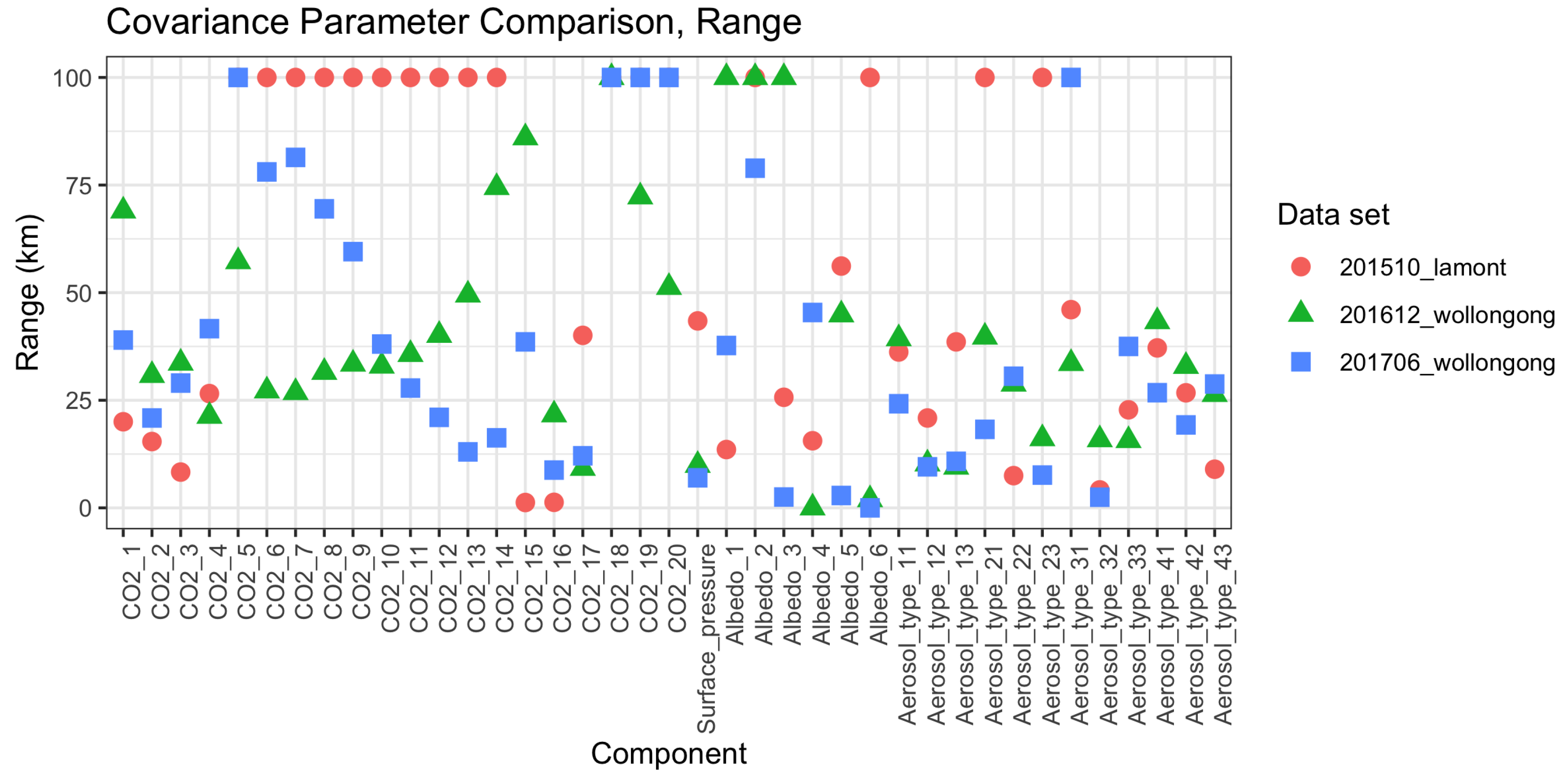
  • Estimate the spatial correlation parameters λ k and ν k from the OCO-2 retrievals, one state vector element at a time.
The above procedure has the practical advantage that the available data align exactly with the necessary structure of the state vector and the desired spatial resolution. However, the OCO-2 data products will still have incomplete information about the underlying physical mechanisms driving spatial correlations. Alternative sources for estimation would include transport models.

References

  1. Kuze, A.; Suto, H.; Nakajima, M.; Hamazaki, T. Thermal and near infrared sensor for carbon observation Fourier-transform spectrometer on the Greenhouse Gases Observing Satellite for greenhouse gases monitoring. Appl. Opt. 2009, 48, 6716–6733. [Google Scholar] [CrossRef] [PubMed]
  2. Eldering, A.; O’Dell, C.W.; Wennberg, P.O.; Crisp, D.; Gunson, M.; Viatte, C.; Avis, C.; Braverman, A.; Castano, R.; Chang, A.; et al. The Orbiting Carbon Observatory-2: First 18 months of science data products. Atmos. Meas. Tech. 2017, 10, 549–563. [Google Scholar] [CrossRef] [Green Version]
  3. Crowell, S.; Baker, D.; Schuh, A.; Basu, S.; Jacobson, A.R.; Chevallier, F.; Liu, J.; Deng, F.; Feng, L.; McKain, K.; et al. The 2015–2016 carbon cycle as seen from OCO-2 and the global in situ network. Atmos. Chem. Phys. 2019, 19, 9797–9831. [Google Scholar] [CrossRef] [Green Version]
  4. Eldering, A.; Taylor, T.E.; O’Dell, C.W.; Pavlick, R. The OCO-3 mission: Measurement objectives and expected performance based on 1 year of simulated data. Atmos. Meas. Tech. 2019, 12, 2341–2370. [Google Scholar] [CrossRef] [Green Version]
  5. Miller, C.E.; Crisp, D.; DeCola, P.L.; Olsen, S.C.; Randerson, J.T.; Michalak, A.M.; Alkhaled, A.; Rayner, P.; Jacob, D.J.; Suntharalingam, P.; et al. Precision requirements for space-based data. J. Geophys. Res. Atmos. 2007, 112. [Google Scholar] [CrossRef]
  6. Chevallier, F.; Bréon, F.M.; Rayner, P.J. Contribution of the Orbiting Carbon Observatory to the estimation of CO2 sources and sinks: Theoretical study in a variational data assimilation framework. J. Geophys. Res. Atmos. 2007, 112. [Google Scholar] [CrossRef]
  7. Cressie, N. Mission CO2ntrol: A statistical scientist’s role in remote sensing of atmospheric carbon dioxide. J. Am. Stat. Assoc. 2018, 113, 152–168. [Google Scholar] [CrossRef] [Green Version]
  8. Rodgers, C.D. Inverse Methods for Atmospheric Sounding; World Scientific: Hackensack, NJ, USA, 2000. [Google Scholar]
  9. O’Dell, C.W.; Connor, B.; Boesch, H.; O’Brien, D.; Frankenberg, C.; Castano, R.; Eldering, A.; Fisher, B.; Gunson, M.; McDuffie, J.; et al. The ACOS CO2 retrieval algorithm–Part 1: Description and validation against synthetic observations. Atmos. Meas. Tech. 2012, 5, 99–121. [Google Scholar] [CrossRef] [Green Version]
  10. O’Dell, C.W.; Eldering, A.; Wennberg, P.O.; Crisp, D.; Gunson, M.R.; Fisher, B.; Frankenberg, C.; Kiel, M.; Lindqvist, H.; Mandrake, L.; et al. Improved Retrievals of Carbon Dioxide from the Orbiting Carbon Observatory-2 with the version 8 ACOS algorithm. Atmos. Meas. Tech. 2018, 11, 6539–6576. [Google Scholar] [CrossRef] [Green Version]
  11. Wunch, D.; Toon, G.C.; Blavier, J.F.L.; Washenfelder, R.A.; Notholt, J.; Connor, B.J.; Griffith, D.W.; Sherlock, V.; Wennberg, P.O. The Total Carbon Column Observing Network. Philos. Trans. R. Soc. A 2011, 369. [Google Scholar] [CrossRef] [Green Version]
  12. Worden, J.R.; Doran, G.; Kulawik, S.; Eldering, A.; Crisp, D.; Frankenberg, C.; O’Dell, C.; Bowman, K. Evaluation and Attribution of OCO-2 XCO2 Uncertainties. Atmos. Meas. Tech. 2017, 10, 2759–2771. [Google Scholar] [CrossRef] [Green Version]
  13. Zhang, B.; Cressie, N.; Wunch, D. Inference for Errors-in-Variables Models in the Presence of Spatial and Temporal Dependence with an Application to a Satellite Remote Sensing Campaign. Technometrics 2019, 61, 187–201. [Google Scholar] [CrossRef] [Green Version]
  14. Torres, A.D.; Keppel-Aleks, G.; Doney, S.C.; Fendrock, M.; Luis, K.; Maziére, M.D.; Hase, F.; Petri, C.; Pollard, D.F.; Roehl, C.M.; et al. A Geostatistical Framework for Quantifying the Imprint of Mesoscale Atmospheric Transport on Satellite Trace Gas Retrievals. J. Geophys. Res. 2019, 124. [Google Scholar] [CrossRef] [Green Version]
  15. Dubovik, O.; Herman, M.; Holdak, A.; Lapyonok, T.; Tanré, D.; Deuzé, J.L.; Ducos, F.; Sinyuk, A.; Lopatin, A. Statistically optimized inversion algorithm for enhanced retrieval of aerosol properties from spectral multi-angle polarimetric satellite observations. Atmos. Meas. Tech. 2011, 4, 975–1018. [Google Scholar] [CrossRef] [Green Version]
  16. Xu, F.; Diner, D.J.; Dubovik, O.; Schechner, Y. A correlated multi-pixel inversion approach for aerosol remote sensing. Remote Sens. 2019, 11, 746. [Google Scholar] [CrossRef] [Green Version]
  17. Diner, D.J.; Boland, S.W.; Brauer, M.; Bruegge, C.; Burke, K.A.; Chipman, R.; Di Girolamo, L.; Garay, M.J.; Hasheminassab, S.; Hyer, E.; et al. Advances in multiangle satellite remote sensing of speciated airborne particulate matter and association with adverse health effects: From MISR to MAIA. J. Appl. Remote Sens. 2018, 12, 042603. [Google Scholar] [CrossRef] [Green Version]
  18. Hashimoto, M.; Nakajima, T. Development of a remote sensing algorithm to retrieve atmospheric aerosol properties using multi-wavelength and multi-pixel information. J. Geophys. Res. Atmos. 2017, 122, 6347–6378. [Google Scholar] [CrossRef] [Green Version]
  19. Livesey, N.J.; Van Snyder, W.; Read, W.G.; Wagner, P.A. Retrieval algorithms for the EOS Microwave limb sounder (MLS). IEEE Trans. Geosci. Remote Sens. 2006, 44, 1144–1155. [Google Scholar] [CrossRef]
  20. Hobbs, J.; Braverman, A.; Cressie, N.; Granat, R.; Gunson, M. Simulation-based Uncertainty Quantification for estmating CO2 from satellite data. SIAM/ASA J. Uncertain. Quantif. 2017, 5, 956–985. [Google Scholar] [CrossRef] [Green Version]
  21. Genton, M.G.; Kleiber, W. Cross-Covariance Functions for Multivariate Geostatistics. Stat. Sci. 2015, 30, 147–163. [Google Scholar] [CrossRef]
  22. Stein, M.L. Interpolation of Spatial Data: Some Theory for Kriging; Springer: New York, NY, USA, 1999. [Google Scholar]
  23. Cressie, N.; Wikle, C.K. Statistics for Spatio-Temporal Data; John Wiley & Sons: Hoboken, NJ, USA, 2011. [Google Scholar]
  24. Wang, Y.; Jiang, X.; Yu, B.; Jiang, M. A hierarchical Bayesian approach for aerosol retrieval using MISR data. J. Am. Stat. Assoc. 2013, 108, 483–493. [Google Scholar] [CrossRef]
  25. Yao, S.; Wang, Y.; Yu, B. Efficient aerosol retrieval for Multi-angle Imaging SpectroRadiometer (MISR): A Bayesian approach. arXiv 2017, arXiv:1708.01948. [Google Scholar]
  26. Osterman, G.; Eldering, A.; Avis, C.; Chafin, B.; O’Dell, C.; Frankenberg, C.; Fisher, B.; Mandrake, L.; Wunch, D.; Granat, R.; et al. Orbiting Carbon Observatory-2: Data Product User’s Guide, Operational L1 and L2 Data Versions 8 and Lite File Version 9. 2018. Available online: https://docserver.gesdisc.eosdis.nasa.gov/public/project/OCO/OCO2_DUG.V9.pdf (accessed on 3 March 2020).
  27. Nassar, R.; Hill, T.G.; McLinden, C.A.; Wunch, D.; Jones, D.B.A.; Crisp, D. Quantifying CO2 Emissions From Individual Power Plants From Space. Geophys. Res. Lett. 2017, 44. [Google Scholar] [CrossRef] [Green Version]
  28. Diallo, M.; Legras, B.; Ray, E.; Engel, A.; Anel, J.A. Global distribution of CO2 in the upper troposphere and stratosphere. Atmos. Chem. Phys. 2017, 17, 3861–3878. [Google Scholar] [CrossRef] [Green Version]
  29. Chevallier, F.; Broquet, G.; Pierangelo, C.; Crisp, D. Probabilistic global maps of the CO2 column at daily and monthly scales from sparse satellite measurements. J. Geophys. Res. Atmos. 2017, 122, 7614–7629. [Google Scholar] [CrossRef]
  30. Nguyen, H.; Cressie, N.; Hobbs, J. Sensitivity of Optimal Estimation satellite retrievals to misspecification of the prior mean and covariance, with application to OCO-2 retrievals. Remote Sens. 2019, 11, 2770. [Google Scholar] [CrossRef] [Green Version]
  31. Gneiting, T.; Katzfuss, M. Probabilistic forecasting. Annu. Rev. Stat. Its Appl. 2014, 1, 125–151. [Google Scholar] [CrossRef]
  32. Jacobs, N.; Simpson, W.R.; Wunch, D.; O’Dell, C.W.; Osterman, G.B.; Hase, F.; Blumenstock, T.; Tu, Q.; Frey, M.; Dubey, M.K.; et al. Quality controls, bias, and seasonality of CO2 columns in the boreal forest with Orbiting Carbon Observatory-2, Total Carbon Column Observing Network, and EM27/SUN measurements. Atmos. Meas. Tech. 2020, 13, 5033–5063. [Google Scholar] [CrossRef]
  33. Wunch, D.; Wennberg, P.O.; Osterman, G.; Fisher, B.; Naylor, B.; Roehl, C.M.; O’Dell, C.; Mandrake, L.; Viatte, C.; Kiel, M.; et al. Comparisons of the Orbiting Carbon Observatory-2 (OCO-2) XCO2 measurements with TCCON. Atmos. Meas. Tech. 2017, 10, 2209–2238. [Google Scholar] [CrossRef] [Green Version]
  34. Chevallier, F. On the statistical optimality of CO2 atmospheric inversions assimilating CO2 column retrievals. Atmos. Chem. Phys. 2015, 15, 11133–11145. [Google Scholar] [CrossRef] [Green Version]
  35. Paciorek, C.; Schervish, M. Spatial modelling using a new class of nonstationary covariance functions. Environmetrics 2006, 17, 483–506. [Google Scholar] [CrossRef] [PubMed]
  36. Stein, M.L. Nonstationary Spatial Covariance Functions; Technical Report No. 21; University of Chicago: Chicago, IL, USA, 2005. [Google Scholar]
  37. Kulawik, S.S.; O’Dell, C.; Nelson, R.R.; Taylor, T.E. Validation of OCO-2 error analysis using simulated retrievals. Atmos. Meas. Tech. 2019, 12, 5317–5334. [Google Scholar] [CrossRef] [Green Version]
  38. Higham, N. Computing the nearest correlation matrix—A problem from finance. IMA J. Numer. Anal. 2002, 22, 329–343. [Google Scholar] [CrossRef] [Green Version]
  39. Bates, D.; Maechler, M. Matrix: Sparse and Dense Matrix Classes and Methods; R Package Version 1.2-18; R Foundation for Statistical Computing: Vienna, Austria, 2019. [Google Scholar]
Figure 1. Left: Portion of an Orbiting Carbon Observatory-2 (OCO-2) orbit representing a small area for which a spatial retrieval is investigated. The area in green represents the small area. Right: Zoomed-in view of the locations of the centers of n = 64 individual footprints for the small area.
Remotesensing 13 00571 g001
Figure 2. Estimated Matérn spatial correlation range parameters in kilometers for all state vector elements in three Total Carbon Column Observing Network (TCCON) templates. Estimates have been truncated above at 100 km.
Remotesensing 13 00571 g002
Figure 3. True mean vectors μ T and operational retrieval prior mean vectors μ a for the CO2 vertical profile at the three TCCON templates.
Remotesensing 13 00571 g003
Figure 4. Log mean squared error (MSE) for the retrieval error of the state vector components, averaged across 100 samples and 64 locations per sample. State vector elements are grouped into the CO2 vertical profile (top) and all other elements (bottom). All results are for the October 2015 Lamont template.
Remotesensing 13 00571 g004
Figure 5. Example of pointwise 95% posterior credible intervals for XCO2 (in ppm) at a subset of the 64 locations for the October 2015 Lamont template. For spatial retrievals, the posterior intervals were narrower and centered closer to the true XCO2 values.
Remotesensing 13 00571 g005
Figure 6. XCO2 retrieval error correlations across locations for 100 samples for the October 2015 Lamont template. Typical operational priors lead to predictions with errors that have strong spatial correlation.
Remotesensing 13 00571 g006
Figure 7. Mean absolute error (MAE) for XCO2 (in ppm) across locations for 100 samples for the October 2015 Lamont template for retrievals using the spatial prior.
Remotesensing 13 00571 g007
Table 1. Elements of the state vector for the reduced-order model of [20].
CollectionNumber of Elements
CO2 Vertical Profile20
Surface Pressure1
Surface Albedo6 = 2 per band × 3 bands
Aerosols12 = 3 per type × 4 types
Table 2. True mean vectors μ T and operational retrieval prior mean vectors μ a for selected state vector elements at the three TCCON templates. The CO2 profile means are displayed in Figure 3. Aerosols are represented with two location-specific types plus cloud ice and water.
LamontWollongongWollongong
Oct 2015Dec 2016Jun 2017
State Vector Element μ T μ a μ T μ a μ T μ a
XCO2 [ppm]396.34395.72398.84400.76399.98402.02
Surface Pressure [hPa]986.36983.60949.81945.89953.18952.27
Strong CO2 Mean Albedo0.1940.1180.1470.1830.1330.097
Strong CO2 Albedo Slope 8.05 × 10 5 0 1.06 × 10 4 0 1.80 × 10 5 0
Weak CO2 Mean Albedo0.2040.1930.2130.2230.2120.231
Weak CO2 Albedo Slope 2.49 × 10 5 0 2.52 × 10 5 0 2.25 × 10 5 0
O2 A-Band Mean Albedo0.3000.2580.2610.3380.2520.232
O2 A-Band Albedo Slope 1.43 × 10 4 0 1.15 × 10 4 0 1.63 × 10 4 0
Aerosol Type 1SulfateSulfateSulfate
   Log Optical Depth−3.72−3.72−4.26−4.09−4.80−4.89
   Profile Height0.830.900.790.900.930.90
   Log Profile Thickness−2.65−3.00−2.32−3.00−3.49−3.00
Aerosol Type 2DustSea SaltSea Salt
   Log Optical Depth−6.13−4.72−5.27−4.11−5.36−4.95
   Profile Height0.720.900.820.900.910.90
   Log Profile Thickness−2.50−3.00−3.19−3.00−3.76−3.00
Cloud Ice
   Log Optical Depth−5.26−4.38−5.16−4.38−5.90−4.38
   Profile Height0.170.150.230.160.010.20
   Log Profile Thickness−3.22−3.22−3.22−3.22−3.22−3.22
Cloud Water
   Log Optical Depth−5.13−4.38−4.89−4.38−5.10−4.38
   Profile Height0.860.750.860.751.080.75
   Log Profile Thickness−2.30−2.30−2.30−2.30−2.30−2.30
Table 3. Performance of multiple retrieval approaches from three simulation experiments. The joint and marginal log scores are defined in Equations (3) and (4) and summarize the retrieval of XCO2. The mean squared error (MSE) is shown for XCO2 and the full state vector, as well as the mean absolute error (MAE) for the full state vector. Results in bold indicate the optimal performance for each metric.
XCO2Full State
SiteMethodMarginal Log ScoreJoint Log ScoreMSEMAEMSE
LamontTrue−1318−Inf0.460.730.75
Oct 2015Operational−90−900.630.510.62
Spatial−22250.030.240.27
WollongongTrue−44863−Inf16.074.724.74
Dec 2016Operational−87−870.880.760.78
Spatial−23120.110.430.46
WollongongTrue−11818−Inf6.253.023.12
Jun 2017Operational−61−610.200.530.56
Spatial−120.20.040.440.48
Publisher’s Note: MDPI stays neutral with regard to jurisdictional claims in published maps and institutional affiliations.

