
Mapping and Characterization of Phenological Changes over Various Farming Systems in an Arid and Semi-Arid Region Using Multitemporal Moderate Spatial Resolution Data

 , ,
, ,  ,
,
Abstract
:
1. Introduction
2. Materials and Methods
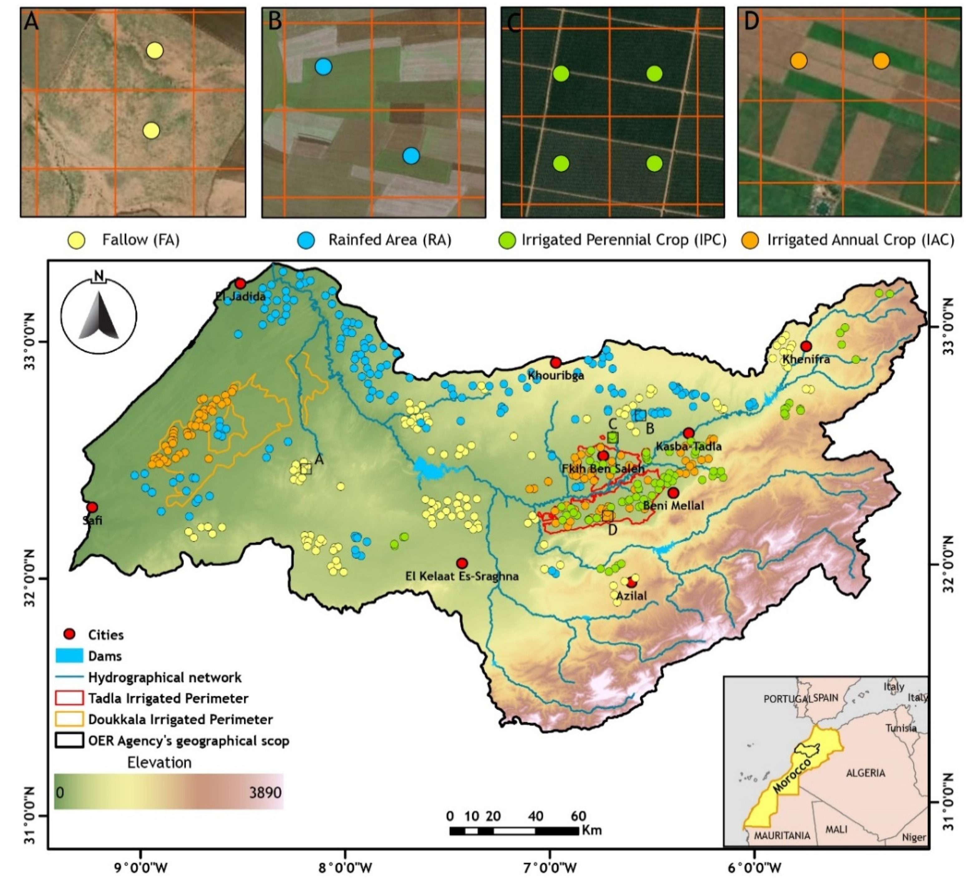
2.1. Study Area
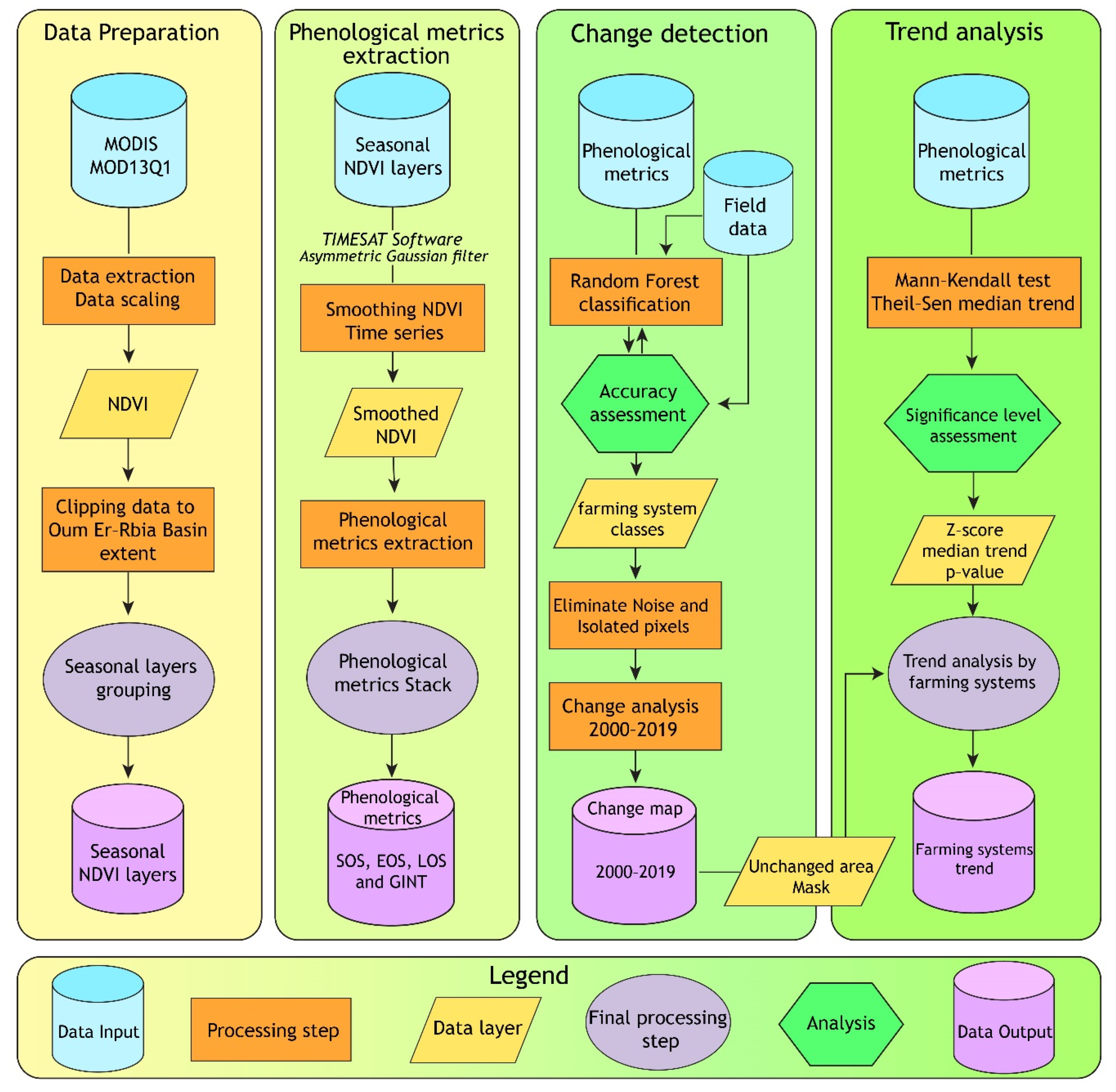
2.2. Multitemporal MODIS and CHIRPS Data Acquisition and Derived NDVI Processing
2.3. Statistical Analysis
2.3.1. Random Forest Classification and Change Analysis
2.3.2. Variability and Trend Analysis
3. Results
3.1. NDVI and Rainfall Time Series Analysis
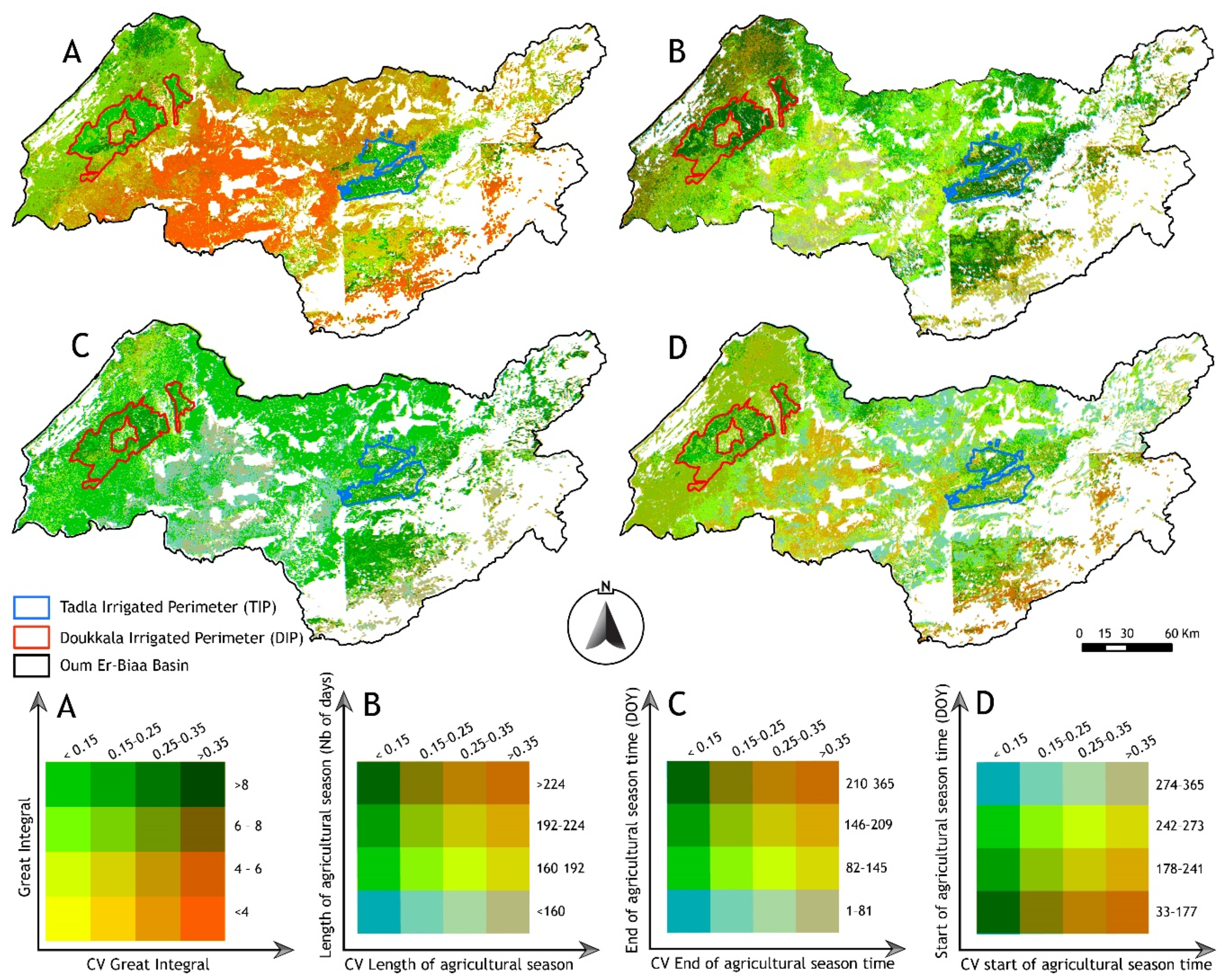
3.2. Spatial Patterns of Phenological Metrics
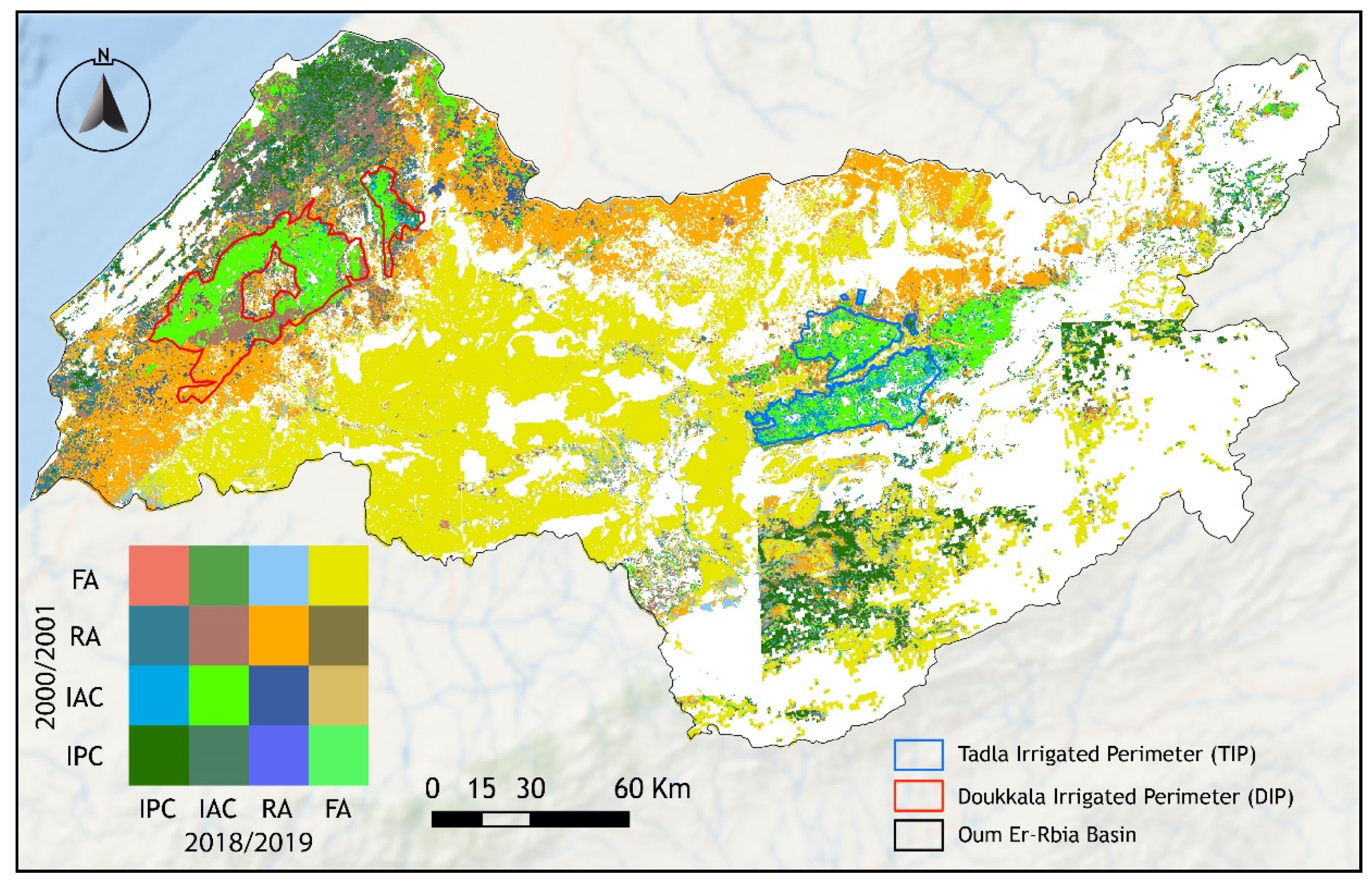
3.3. Determination of Unchanged Farming Systems’ Area
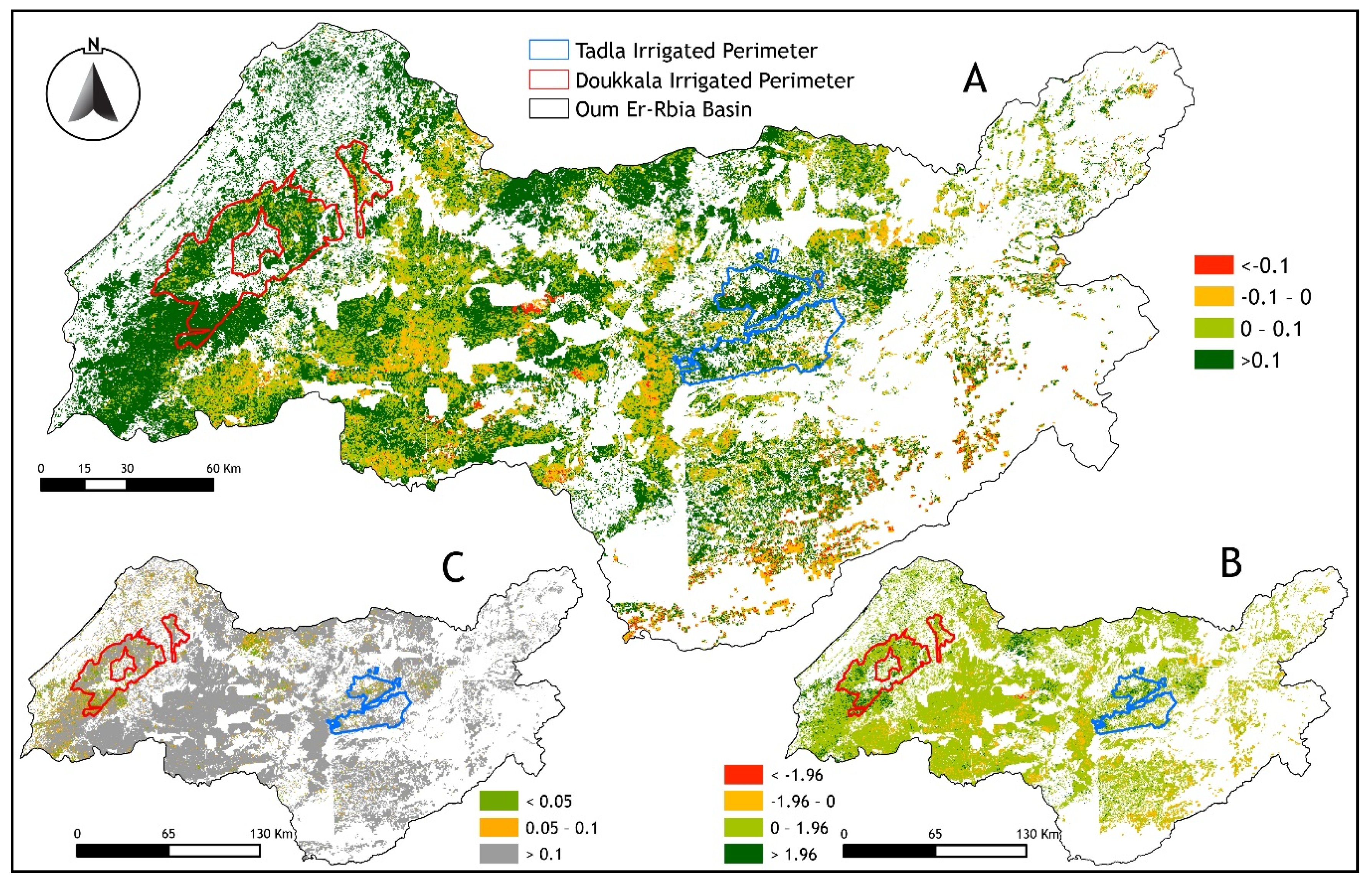
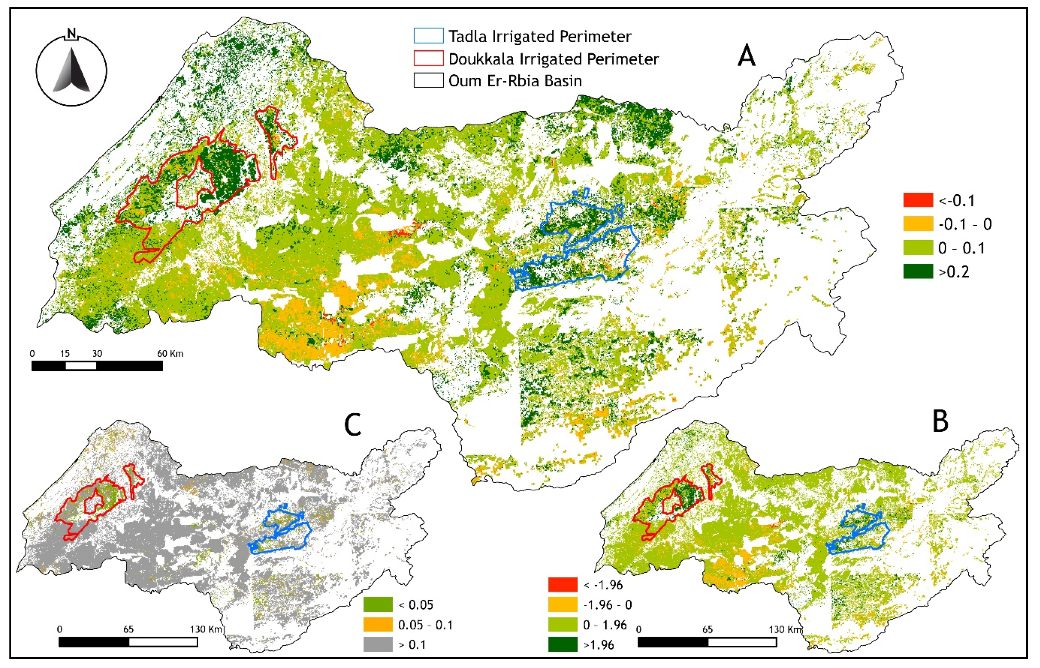
3.4. Trend Analysis Results
4. Discussion
5. Conclusions
Supplementary Materials
Author Contributions
Funding
Institutional Review Board Statement
Informed Consent Statement
Data Availability Statement
Acknowledgments
Conflicts of Interest
References
- Lionboui, H.; Benabdelouahab, T.; Htitiou, A.; Lebrini, Y.; Boudhar, A.; Hadria, R.; Elame, F.; AbdelGhani, B. Spatial assessment of losses in wheat production value: A need for an innovative approach to guide risk management policies. Remote. Sens. Appl. Soc. Environ. 2020, 18, 100300. [Google Scholar] [CrossRef]
- Benabdelouahab, T.; Lebrini, Y.; Boudhar, A.; Hadria, R.; Htitiou, A.; Lionboui, H. Monitoring spatial variability and trends of wheat grain yield over the main cereal regions in Morocco: A remote-based tool for planning and adjusting policies. Geocarto Int. 2019. [Google Scholar] [CrossRef]
- Sishodia, R.P.; Ray, R.L.; Singh, S.K. Applications of Remote Sensing in Precision Agriculture: A Review. Remote. Sens. 2020, 12, 3136. [Google Scholar] [CrossRef]
- Lebrini, Y.; Boudhar, A.; Htitiou, A.; Hadria, R.; Lionboui, H.; Bounoua, L.; Benabdelouahab, T. Remote monitoring of agricultural systems using NDVI time series and machine learning methods: A tool for an adaptive agricultural policy. Arab. J. Geosci. 2020, 13, 1–14. [Google Scholar] [CrossRef]
- Atzberger, C.; Klisch, A.; Mattiuzzi, M.; Vuolo, F. Phenological Metrics Derived over the European Continent from NDVI3g Data and MODIS Time Series. Remote. Sens. 2013, 6, 257–284. [Google Scholar] [CrossRef] [Green Version]
- Schreier, J.; Ghazaryan, G.; Dubovyk, O. Crop-specific phenomapping by fusing Landsat and Sentinel data with MODIS time series. Eur. J. Remote. Sens. 2020, 1, 1–12. [Google Scholar] [CrossRef]
- Benabdelouahab, T.; Balaghi, R.; Hadria, R.; Lionboui, H.; Minet, J.; Tychon, B. Monitoring surface water content using visible and short-wave infrared SPOT-5 data of wheat plots in irrigated semi-arid regions. Int. J. Remote. Sens. 2015, 36, 4018–4036. [Google Scholar] [CrossRef]
- Benabdelouahab, T.; Dominique, D.; Hayat, L.; Rachid, H.; Bernard, T.; Abdelghani, B.; Riad, B.; Youssef, L.; Hamid, M.; Christian, B. Using SAR Data to Detect Wheat Irrigation Supply in an Irrigated Semi-arid Area. J. Agric. Sci. 2018, 11, 1916–9760. [Google Scholar] [CrossRef]
- Hentze, K.; Thonfeld, F.; Menz, G. Evaluating Crop Area Mapping from MODIS Time-Series as an Assessment Tool for Zimbabwe’s “Fast Track Land Reform Programme”. PLoS ONE 2016, 11, e0156630. [Google Scholar] [CrossRef]
- Li, L.; Friedl, M.A.; Xin, Q.; Gray, J.; Pan, Y.; Frolking, S. Mapping Crop Cycles in China Using MODIS-EVI Time Series. Remote. Sens. 2014, 6, 2473–2493. [Google Scholar] [CrossRef] [Green Version]
- Lu, D.; Mausel, P.; Brondízio, E.; Moran, E. Change detection techniques. Int. J. Remote. Sens. 2004, 25, 2365–2401. [Google Scholar] [CrossRef]
- Coppin, P.J.I.; Nackaerts, K.; Muys, B.; Lambin, E. Digital change detection methods in ecosystem monitoring: A review. Int. J. Remote Sens. 2004, 25, 1565–1596. [Google Scholar] [CrossRef]
- Salhi, A.; Benabdelouahab, T.; Martin-Vide, J.; Okacha, A.; El Hasnaoui, Y.; El Mousaoui, M.; El Morabit, A.; Himi, M.; Benabdelouahab, S.; Lebrini, Y.; et al. Bridging the gap of perception is the only way to align soil protection actions. Sci. Total. Environ. 2020, 718, 137421. [Google Scholar] [CrossRef] [PubMed]
- Htitiou, A.; Boudhar, A.; Lebrini, Y.; Hadria, R.; Lionboui, H.; Elmansouri, L.; Tychon, B.; Benabdelouahab, T. The Performance of Random Forest Classification Based on Phenological Metrics Derived from Sentinel-2 and Landsat 8 to Map Crop Cover in an Irrigated Semi-arid Region. Remote. Sens. Earth Syst. Sci. 2019, 2, 208–224. [Google Scholar] [CrossRef]
- Htitiou, A.; Boudhar, A.; Lebrini, Y.; Hadria, R.; Lionboui, H.; Benabdelouahab, T. A comparative analysis of different phenological information retrieved from Sentinel-2 time series images to improve crop classification: A machine learning approach. Geocarto Int. 2020, 1–24. [Google Scholar] [CrossRef]
- Cleland, E.E.; Chuine, I.; Menzel, A.; Mooney, H.A.; Schwartz, M.D. Shifting plant phenology in response to global change. Trends Ecol. Evol. 2007, 22, 357–365. [Google Scholar] [CrossRef]
- Moulin, S.; Kergoat, L.; Viovy, N.; Dedieu, G. Global-Scale Assessment of Vegetation Phenology Using NOAA/AVHRR Satellite Measurements. J. Clim. 1997, 10, 1154–1170. [Google Scholar] [CrossRef]
- Zhou, L.; Tucker, C.; Kaufmann, R.K.; Slayback, D.; Shabanov, N.V.; Myneni, R. Variations in northern vegetation activity inferred from satellite data of vegetation index during 1981 to 1999. J. Geophys. Res. Atmos. 2001, 106, 20069–20083. [Google Scholar] [CrossRef]
- Castro, C.L.; Beltrán-Przekurat, A.B.; Pielke, R.A. Spatiotemporal Variability of Precipitation, Modeled Soil Moisture, and Vegetation Greenness in North America within the Recent Observational Record. J. Hydrometeorol. 2009, 10, 1355–1378. [Google Scholar] [CrossRef] [Green Version]
- Hanamean, J.R., Jr.; Pielke, R.A., Sr.; Castro, C.L.; Ojima, D.S.; Reed, B.C.; Gao, Z. Vegetation greenness impacts on maximum and minimum temperatures in northeast Colorado. Meteorol. Appl. 2003, 10, 203–215. [Google Scholar] [CrossRef] [Green Version]
- White, M.A.; De Beurs, K.M.; Didan, K.; Inouye, D.W.; Richardson, A.D.; Jensen, O.P.; O’Keefe, J.; Zhang, G.; Nemani, R.R.; Van Leeuwen, W.J.D.; et al. Intercomparison, interpretation, and assessment of spring phenology in North America estimated from remote sensing for 1982–2006. Glob. Chang. Biol. 2009, 15, 2335–2359. [Google Scholar] [CrossRef]
- DeFries, R.S.; Field, C.B.; Fung, I.; Collatz, G.J.; Bounoua, L. Combining satellite data and biogeochemical models to estimate global effects of human-induced land cover change on carbon emissions and primary productivity. Glob. Biogeochem. Cycles 1999, 13, 803–815. [Google Scholar] [CrossRef]
- Adole, T.; Dash, J.; Atkinson, P.M. Characterising the land surface phenology of Africa using 500 m MODIS EVI. Appl. Geogr. 2018, 90, 187–199. [Google Scholar] [CrossRef] [Green Version]
- Chandola, V.; Hui, D.; Gu, L.; Bhaduri, B.; Vatsavai, R.R. Using Time Series Segmentation for Deriving Vegetation Phenology Indices from MODIS NDVI Data. In Proceedings of the IEEE International Conference on Data Mining Workshops, Sydney, NSW, Australia, 13 December 2010; pp. 202–208. [Google Scholar]
- Lebrini, Y.; Boudhar, A.; Hadria, R.; Lionboui, H.; Elmansouri, L.; Arrach, R.; Ceccato, P.; Benabdelouahab, T. Identifying Agricultural Systems Using SVM Classification Approach Based on Phenological Metrics in a Semi-arid Region of Morocco. Earth Syst. Environ. 2019, 3, 277–288. [Google Scholar] [CrossRef]
- Wessels, K.J.; Bachoo, A.; Archibald, S. Influence of composite period and date of observation on phenological metrics ex-tracted from MODIS data. In Proceedings of the 33rd International Symposium on Remote Sensing of Environment: Sustaining the Millennium Development Goals, Stresa, Lago Magglore, Italy, 4–8 May 2009. [Google Scholar]
- Bachoo, A.; Archibald, S. Influence of Using Date-Specific Values when Extracting Phenological Metrics from 8-day Composite NDVI Data. In Proceedings of the 2007 International Workshop on the Analysis of Multi-temporal Remote Sensing Images, Leuven, Belgium, 18–20 July 2007; pp. 1–4. [Google Scholar] [CrossRef] [Green Version]
- Archibald, S.; Scholes, R.J. Leaf green-up in a semi-arid African savanna-separating tree and grass responses to environ-mental cues. J. Veg. Sci. 2007, 18, 583–594. [Google Scholar]
- Schwartz, M.D. Phenology: An Integrative Environmental Science; Kluwer Academic Publishers: Dordrecht, The Netherlands, 2003; p. 564. [Google Scholar]
- Alcantara, C.; Kuemmerle, T.; Prishchepov, A.V.; Radeloff, V.C. Mapping abandoned agriculture with multi-temporal MODIS satellite data. Remote. Sens. Environ. 2012, 124, 334–347. [Google Scholar] [CrossRef]
- Qiu, B.; Lu, D.; Tang, Z.; Song, D.; Zeng, Y.; Wang, Z.; Chen, C.; Chen, N.; Huang, H.; Xu, W. Mapping cropping intensity trends in China during 1982–2013. Appl. Geogr. 2017, 79, 212–222. [Google Scholar] [CrossRef]
- Jönsson, P.; Cai, Z.; Melaas, E.; Friedl, M.A.; Eklundh, L. A Method for Robust Estimation of Vegetation Seasonality from Landsat and Sentinel-2 Time Series Data. Remote. Sens. 2018, 10, 635. [Google Scholar] [CrossRef] [Green Version]
- Bai, Y.; Yang, Y.; Jiang, H. Intercomparison of AVHRR GIMMS3g, Terra MODIS, and SPOT-VGT NDVI Products over the Mongolian Plateau. Remote. Sens. 2019, 11, 2030. [Google Scholar] [CrossRef] [Green Version]
- Lebrini, Y.; Benabdelouahab, T.; Boudhar, A.; Htitiou, A.; Hadria, R.; Lionboui, H. Farming systems monitoring using machine learning and trend analysis methods based on fitted NDVI time series data in a semi-arid region of Morocco. In Proceedings of the Remote Sensing for Agriculture, Ecosystems, and Hydrology XXI, Strasbourg, France, 9–11 September 2019; Volume 11149. [Google Scholar] [CrossRef]
- Suepa, T.; Qi, J.; Lawawirojwong, S.; Messina, J.P. Understanding spatio-temporal variation of vegetation phenology and rainfall seasonality in the monsoon Southeast Asia. Environ. Res. 2016, 147, 621–629. [Google Scholar] [CrossRef] [Green Version]
- Wang, D.; Wan, B.; Qiu, P.; Su, Y.; Guo, Q.; Wang, R.; Sun, F.; Wu, X. Evaluating the Performance of Sentinel-2, Landsat 8 and Pléiades-1 in Mapping Mangrove Extent and Species. Remote. Sens. 2018, 10, 1468. [Google Scholar] [CrossRef] [Green Version]
- Wessel, M.; Brandmeier, M.; Tiede, D. Evaluation of Different Machine Learning Algorithms for Scalable Classification of Tree Types and Tree Species Based on Sentinel-2 Data. Remote. Sens. 2018, 10, 1419. [Google Scholar] [CrossRef] [Green Version]
- Yu, L.; Su, J.; Li, C.; Wang, L.; Luo, Z.; Yan, B. Improvement of Moderate Resolution Land Use and Land Cover Classification by Introducing Adjacent Region Features. Remote. Sens. 2018, 10, 414. [Google Scholar] [CrossRef] [Green Version]
- Breiman, L. Random Forests. Mach. Learn. 2001, 45, 5–32. [Google Scholar] [CrossRef] [Green Version]
- Jin, Y.; Sung, S.; Lee, D.K.; Biging, G.S.; Jeong, S. Mapping Deforestation in North Korea Using Phenology-Based Multi-Index and Random Forest. Remote. Sens. 2016, 8, 997. [Google Scholar] [CrossRef] [Green Version]
- James, G.; Witten, D.; Hastie, T.; Tibshirani, R. An Introduction to Statistical Learning: With Applications in R; Springer: New York, NY, USA, 2014. [Google Scholar]
- Ouatiki, H.; Boudhar, A.; Ouhinou, A.; Beljadid, A.; Leblanc, M.J.; Chehbouni, A. Sensitivity and Interdependency Analysis of the HBV Conceptual Model Parameters in a Semi-Arid Mountainous Watershed. Water 2020, 12, 2440. [Google Scholar] [CrossRef]
- Boudhar, A.; Ouatiki, H.; Bouamri, H.; Lebrini, Y.; Karaoui, I.; Hssaisoune, M.; Arioua, A.; Benabdelouahab, T. Hydro-logical Response to Snow Cover Changes Using Remote Sensing over the Oum Er Rbia Upstream Basin, Morocco; Rebai, N., Mastere, M., Eds.; Springer: Berlin/Heidelberg, Germany, 2020; pp. 95–102. [Google Scholar]
- CHIRPS. Available online: https://www.chc.ucsb.edu/data/chirps (accessed on 13 May 2020).
- Jönsson, P.; Eklundh, L. TIMESAT—A program for analyzing time-series of satellite sensor data. Comput. Geosci. 2004, 30, 833–845. [Google Scholar] [CrossRef] [Green Version]
- Chen, J.; Jönsson, P.; Tamura, M.; Gu, Z.; Matsushita, B.; Eklundh, L. A simple method for reconstructing a high-quality NDVI time-series data set based on the Savitzky–Golay filter. Remote Sens. Environ. 2004, 91, 332–344. [Google Scholar] [CrossRef]
- Chen, J.; Wilson, W.S.; Seo, K.-W. Optimized smoothing of Gravity Recovery and Climate Experiment (GRACE) time-variable gravity observations. J. Geophys. Res. Space Phys. 2006, 111. [Google Scholar] [CrossRef] [Green Version]
- Geng, L.; Ma, M.; Wang, X.; Yu, W.; Jia, S.; Wang, H. Comparison of Eight Techniques for Reconstructing Multi-Satellite Sensor Time-Series NDVI Data Sets in the Heihe River Basin, China. Remote. Sens. 2014, 6, 2024–2049. [Google Scholar] [CrossRef] [Green Version]
- Jönsson, P.; Eklundh, L. Seasonality extraction by function fitting to time-series of satellite sensor data. IEEE Trans. Geosci. Remote. Sens. 2002, 40, 1824–1832. [Google Scholar] [CrossRef]
- Fu, Y.; He, H.; Zhao, J.-J.; Larsen, D.; Zhang, H.-Y.; Sunde, M.G.; Duan, S. Climate and Spring Phenology Effects on Autumn Phenology in the Greater Khingan Mountains, Northeastern China. Remote. Sens. 2018, 10, 449. [Google Scholar] [CrossRef] [Green Version]
- Gao, F.; Morisette, J.T.; Wolfe, R.E.; Ederer, G.; Pedelty, J.; Masuoka, E.; Myneni, R.; Tan, B.; Nightingale, J. An Algorithm to Produce Temporally and Spatially Continuous MODIS-LAI Time Series. IEEE Geosci. Remote. Sens. Lett. 2008, 5, 60–64. [Google Scholar] [CrossRef]
- Eklundh, L.; Jönsson, P. Timesat 3.2 Software Manual; Lund and Malmö University: Lund, Sweden, 2015. [Google Scholar]
- Eklundh, L.; Jönsson, P. TIMESAT for Processing Time-Series Data from Satellite Sensors for Land Surface Monitoring. In Radar Remote Sensing of Urban Areas; Springer: Berlin/Heidelberg, Germany, 2016; pp. 177–194. [Google Scholar]
- Reed, B.C.; Brown Jesslyn, F.; VanderZee, D.; Loveland, T.R.; Merchant, J.W.; Ohlen, D.O. Measuring phenological varia-bility from satellite imagery. J. Veg. Sci. 1994, 5, 703–714. [Google Scholar] [CrossRef]
- Hadria, R.; Benabdelouahab, T.; Mahyou, H.; Balaghi, R.; Bydekerke, L.; El Hairech, T.; Ceccato, P. Relationships between the three components of air temperature and remotely sensed land surface temperature of agricultural areas in Morocco. Int. J. Remote. Sens. 2018, 39, 356–373. [Google Scholar] [CrossRef]
- R Core Team. R: A Language and Environment for Statistical Computing; R Foundation for Statistical Computing: Vienna, Austria, 2017. [Google Scholar]
- Hao, P.; Zhan, Y.; Wang, L.; Niu, Z.; Shakir, M. Feature Selection of Time Series MODIS Data for Early Crop Classification Using Random Forest: A Case Study in Kansas, USA. Remote. Sens. 2015, 7, 5347–5369. [Google Scholar] [CrossRef] [Green Version]
- Belgiu, M.; Drăguţ, L. Random forest in remote sensing: A review of applications and future directions. ISPRS J. Photogramm. Remote. Sens. 2016, 114, 24–31. [Google Scholar] [CrossRef]
- Immitzer, M.; Atzberger, C.; Koukal, T. Tree Species Classification with Random Forest Using Very High Spatial Resolution 8-Band WorldView-2 Satellite Data. Remote. Sens. 2012, 4, 2661–2693. [Google Scholar] [CrossRef] [Green Version]
- Meyer, H.; Reudenbach, C.; Hengl, T.; Katurji, M.; Nauss, T. Improving performance of spatio-temporal machine learning models using forward feature selection and target-oriented validation. Environ. Model. Softw. 2018, 101, 1–9. [Google Scholar] [CrossRef]
- Kendall, M.G. Rank Correlation Methods; Charles Griffin; Oxford University Press: London, UK, 1975; Volume 35. [Google Scholar]
- Davenport, M.L.; Nicholson, S.E. On the relation between rainfall and the Normalized Difference Vegetation Index for diverse vegetation types in East Africa. Int. J. Remote. Sens. 1993, 14, 2369–2389. [Google Scholar] [CrossRef]
- Barbosa, H.A.; Kumar, T.L.; Paredes, F.; Elliott, S.; Rejas, J.G. Assessment of Caatinga response to drought using Meteosat-SEVIRI Normalized Difference Vegetation Index (2008–2016). ISPRS J. Photogramm. Remote. Sens. 2019, 148, 235–252. [Google Scholar] [CrossRef]
- Lotsch, A.; Friedl, M.A.; Anderson, B.T.; Tucker, C.J. Coupled vegetation-precipitation variability observed from satellite and climate records. Geophys. Res. Lett. 2003, 30. [Google Scholar] [CrossRef]
- Vrieling, A.; De Leeuw, J.; Said, M.Y. Length of Growing Period over Africa: Variability and Trends from 30 Years of NDVI Time Series. Remote. Sens. 2013, 5, 982–1000. [Google Scholar] [CrossRef] [Green Version]
- Lionboui, H.; Benabdelouahab, T.; Hasib, A.; Boulli, A. Analysis of Farms Performance Using Different Sources of Irrigation Water: A Case Study in a Semi-Arid Area. Int. J. Agric. Manag. Dev. 2016, 6, 145–154. [Google Scholar]
- Nitze, I.; Barrett, B.; Cawkwell, F. Temporal optimisation of image acquisition for land cover classification with Random Forest and MODIS time-series. Int. J. Appl. Earth Obs. Geoinf. 2015, 34, 136–146. [Google Scholar] [CrossRef] [Green Version]
- Ouatiki, H.; Boudhar, A.; Ouhinou, A.; Arioua, A.; Hssaisoune, M.; Bouamri, H.; Benabdelouahab, T. Trend analysis of rainfall and drought over the Oum Er-Rbia River Basin in Morocco during 1970–2010. Arab. J. Geosci. 2019, 12, 128. [Google Scholar] [CrossRef]
- Luo, Z.; Yu, S. Spatiotemporal Variability of Land Surface Phenology in China from 2001–2014. Remote. Sens. 2017, 9, 65. [Google Scholar] [CrossRef] [Green Version]
- Yuan, M.; Wang, L.; Lin, A.; Liu, Z.; Qu, S. Variations in land surface phenology and their response to climate change in Yangtze River basin during 1982–2015. Theor. Appl. Clim. 2018, 137, 1659–1674. [Google Scholar] [CrossRef]


| Parameter | Description | Value |
|---|---|---|
| Spike method | Two values: 1 for median filter and 2 for decomposition by Loess | 1 |
| Spike value | Degree of spike removal | 1.8 |
| Amplitude cutoff value | Data with amplitude below this value are masked. | 0.1 |
| Valid data range | Data range of time series to be processed | 0–1 |
| Season parameter | The study area contains one cropping season | 1 |
| Number of envelope iterations | Number of iterations for envelope adaptation | 2 |
| Adaptation strength | Strength of the envelope adaptation | 3 |
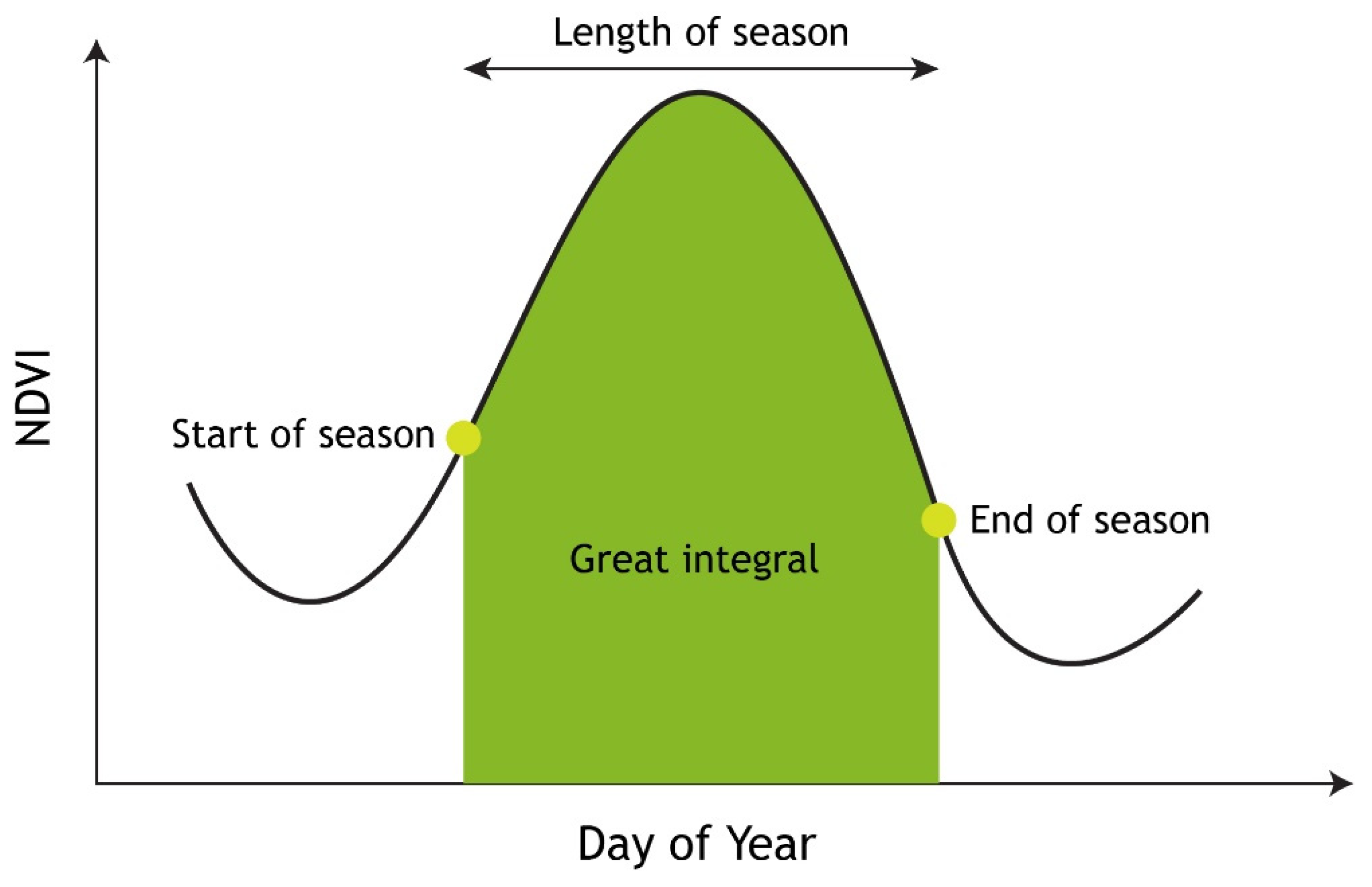
| Phenological Metric | Phenological Definition (for Cropping Season) | Unit |
|---|---|---|
| (1) Start of season—time (TSOS) | Beginning date of photosynthesis activity in the vegetation canopy | days |
| (2) End of season—time (TEOS) | End date of photosynthesis activity in the vegetation canopy | days |
| (3) Length of season (LOS) | Length of photosynthetic activity during the cropping season | days |
| (4) Great integral (GINT) | Canopy photosynthetic activity across the entire growing season | - |
| Farming System Class | Number of Polygons | Training Area (Ha) |
|---|---|---|
| Irrigated Perennial Crop (IPC) | 80 | 1626.71 |
| Irrigated Annual Crop (IAC) | 105 | 1889.12 |
| Rainfed Area (RA) | 160 | 3617.76 |
| Fallow (FA) | 125 | 2661.06 |
| Total | 470 | 9794.65 |
Publisher’s Note: MDPI stays neutral with regard to jurisdictional claims in published maps and institutional affiliations. |
© 2021 by the authors. Licensee MDPI, Basel, Switzerland. This article is an open access article distributed under the terms and conditions of the Creative Commons Attribution (CC BY) license (http://creativecommons.org/licenses/by/4.0/).
Share and Cite
Lebrini, Y.; Boudhar, A.; Laamrani, A.; Htitiou, A.; Lionboui, H.; Salhi, A.; Chehbouni, A.; Benabdelouahab, T. Mapping and Characterization of Phenological Changes over Various Farming Systems in an Arid and Semi-Arid Region Using Multitemporal Moderate Spatial Resolution Data. Remote Sens. 2021, 13, 578. https://doi.org/10.3390/rs13040578
Lebrini Y, Boudhar A, Laamrani A, Htitiou A, Lionboui H, Salhi A, Chehbouni A, Benabdelouahab T. Mapping and Characterization of Phenological Changes over Various Farming Systems in an Arid and Semi-Arid Region Using Multitemporal Moderate Spatial Resolution Data. Remote Sensing. 2021; 13(4):578. https://doi.org/10.3390/rs13040578
Chicago/Turabian StyleLebrini, Youssef, Abdelghani Boudhar, Ahmed Laamrani, Abdelaziz Htitiou, Hayat Lionboui, Adil Salhi, Abdelghani Chehbouni, and Tarik Benabdelouahab. 2021. "Mapping and Characterization of Phenological Changes over Various Farming Systems in an Arid and Semi-Arid Region Using Multitemporal Moderate Spatial Resolution Data" Remote Sensing 13, no. 4: 578. https://doi.org/10.3390/rs13040578